A variational approach to approximate particle number projection with effective forces.

Abstract

Kamlah’s second order method for approximate particle number projection is applied for the first time to variational calculations with effective forces. High spin states of normal and superdeformed nuclei have been calculated with the finite range density dependent Gogny force for several nuclei. Advantages and drawbacks of the Kamlah second order method as compared to the Lipkin-Nogami recipe are thoroughly discussed. We find that the Lipkin Nogami prescription occasionally may fail to find the right energy minimum in the strong pairing regime and that Kamlah’s second order approach though providing better results than the LN one may break down in some limiting situations.

1 Introduction

In recent years it has become clear that a proper treatment of pairing correlations is required to describe many nuclear properties. In particular, in situations of weak pairing one has to go beyond the mean field approximation. Since exact particle number projection (PNP) is very time consuming for non-separable interactions, the approximation most widely used is the Lipkin-Nogami (LN) [1, 2, 3, 4] one, just because of simplicity. The LN prescription can be derived in several ways [5], one transparent derivation [6, 7] can be obtained in terms of the Kamlah [8] expansion to second order. Here one sees that the basic assumptions are : first, to have a well pair-correlated system (i.e. a large particle number fluctuation $\langle(\Delta\hat{N})^{2}\rangle$) and second, to keep constant during the energy minimization procedure, the coefficient ($h_{2}$) of the particle number fluctuation term of the energy expansion. To maintain $h_{2}$ constant amounts to violate the Ritz variational principle, this has advantages and drawbacks. As we shall see, keeping $h_{2}$ constant amounts to stay in the pair-correlated regime, i.e. large $\langle(\Delta\hat{N})^{2}\rangle$, ensuring thereby a good convergence of the Kamlah expansion. On the other hand the lack of variational character may cause to end up in the wrong minimum. The restriction of keeping $h_{2}$ constant can be released and one ends up with a full variational problem, what we shall call the selfconsistent Kamlah approximation to second order (SCK2). In principle, a full variational approach to the problem seems to be the optimal one. Under some conditions, however, it may not be a good approximation because the variation of $h_{2}$ may lead to regions of the Hilbert space with small $\langle(\Delta\hat{N})^{2}\rangle$ values, making the Kamlah expansion to break down.

The validity of both approaches has motivated some interest. Zheng, Sprung and Flocard [5], using a very simple model space of two levels discussed the LN and SCK2 approximation to particle number projection. The force used in the calculations was a monopole pairing which intensity $G$ could be varied in order to simulate different pairing regimes. The energies obtained by means of the two approximate methods were compared with the exact solutions. As a result, it was stated that both methods display an excellent agreement with the exact solution in the regimes of strong and medium pairing correlations. In the regime of weak correlations, however, both theories provided energies deeper than the exact one, the LN approach remaining closer, in general, to the exact value than the SCK2 approach. In a comment to this article, Dobaczewski and Nazarewicz [9] discussed further on the problem. In particular, they explained the strange behavior of the energies in the weak-pairing regime in terms of a violation of the domain of applicability of a quadratic approximation in this regime. It is not obvious that the findings with the exact soluble models will apply to Hamiltonians with more degrees of freedom.

The purpose of this paper is to investigate the LN approach and the fully variational Kamlah method, SCK2, with effective forces and large configurations spaces to analyze under which conditions these approaches are a good approximation to exact particle number projection. We shall furthermore analyze the consistency of the Kamlah expansion. In the numerical application we have solved the LN and SCK2 equations with the finite range density dependent Gogny force [10]. We think that the Gogny force is the ideal one to study these effects because, at variance with the Skyrme and separable forces, in addition to the particle-hole interaction its finite range provides also the particle-particle interaction. In the calculations we shall look for situations where the plain mean field approach is not expected to provide a good description, as high spin states and superdeformed states.

2 Theoretical approximations

In order to discuss the approximations involved in the LN prescription and in the SCK2 approach we shall make a short derivation of the theory [11, 6, 7]. In the case of large particle number violating HFB wave functions $|\Phi\rangle$, i.e. large $\langle(\Delta\hat{N})^{2}\rangle$, with $\Delta\hat{N}=\hat{N}-\langle\Phi|\hat{N}|\Phi\rangle$ and $\langle\hat{N}\rangle\equiv\langle\Phi|\hat{N}|\Phi\rangle$, one may use the Kamlah expansion to calculate the PNP energy. The projected energy to second order is given by

$$E^{(2)}_{proj}\;=\;\langle\hat{H}\rangle\;\;-\;\;h_{2}\langle(\Delta\hat{N})^{2}\rangle\;\;+\;\;h_{1}\;(N_{0}-\langle\hat{N}\rangle)\;\;+\;\;h_{2}\;(N_{0}-\langle\hat{N}\rangle)^{2},$$ (1)

and the coefficients $h_{1},h_{2}$ by

$$h_{1} = \frac{\langle\hat{H}\Delta\hat{N}\rangle-h_{2}\;\langle(\Delta\hat{N})^{3}\rangle}{\langle(\Delta\hat{N})^{2}\rangle}$$ (2)

$$h_{2} = \frac{\langle(\hat{H}-\langle\hat{H}\rangle)(\Delta\hat{N})^{2}\rangle-\langle\hat{H}\Delta\hat{N}\rangle\langle(\Delta\hat{N})^{3}\rangle/\langle(\Delta\hat{N})^{2}\rangle}{\langle(\Delta\hat{N})^{4}\rangle-\langle(\Delta\hat{N})^{2}\rangle^{2}-\langle(\Delta\hat{N})^{3}\rangle^{2}/\langle(\Delta\hat{N})^{2}\rangle}.$$ (3)

The expressions above are valid for one kind of nucleons. In the general case we have $h_{1}^{p},h_{1}^{n}$ and $h_{2}^{p},h_{2}^{n}$ for protons and neutrons. In a full variation after projection method one should vary $E^{(2)}_{proj}$. As an approximation to this method, in order to avoid to compute cumbersome expressions like $\frac{\delta h_{2}}{\delta\Phi}$ one has used the Lipkin-Nogami prescription in which the coefficient $h_{2}$ is held constant during the variation. As a result the LN variational equation is much simpler, one gets

$$\frac{\delta}{\delta\Phi}\langle\hat{H}\rangle-h_{1}\frac{\delta}{\delta\Phi}\langle\hat{N}\rangle+(N_{0}-\langle\hat{N}\rangle)\frac{\delta h_{1}}{\delta\Phi}-2h_{2}(N_{0}-\langle\hat{N}\rangle)\frac{\delta}{\delta\Phi}\langle\hat{N}\rangle-h_{2}\frac{\delta}{\delta\Phi}\langle(\Delta\hat{N})^{2}\rangle=0.$$ (4)

It is obvious that the solution to this equation is equivalent to solve

$$\frac{\delta}{\delta\Phi}\langle\hat{H}-h_{2}(\Delta\hat{N})^{2}\rangle-\lambda\frac{\delta}{\delta\Phi}\langle\hat{N}\rangle=0,$$ (5)

with $\lambda$ determined by the constraint

$$\langle\hat{N}\rangle=N_{0},$$ (6)

provided the condition $\lambda=h_{1}$ is accomplished. This can be easily checked noticing that eq. (5) must hold for any variation $|\delta\Phi\rangle$. In particular, we can choose $|\delta\Phi\rangle=\Delta\hat{N}|\Phi\rangle$, the substitution of this specific variation in eq. (5) provides

$$\langle\hat{H}\Delta\hat{N}\rangle-\lambda\langle(\Delta\hat{N})^{2}\rangle-h_{2}\langle(\Delta\hat{N})^{3}\rangle=0,$$ (7)

comparison with eq. (2) shows that $\lambda=h_{1}$. In the Lipkin-Nogami approach though $h_{2}$ is not varied during the minimization process it is updated in each iteration of the minimization process.

If $h_{2}$ is allowed to vary, the variational principle on $E_{proj}^{(2)}$ is not anymore equivalent to minimize eq. (5) with the constraint on the particle number, because in this case $\lambda\neq h_{1}$. We can, of course, content ourselves with a restricted variation in the Hilbert space. For instance, we can restrict the variational Hilbert space to wave functions $|\Phi\rangle$ satisfying $\langle\Phi|\hat{N}|\Phi\rangle=N_{0}$. In this case the solution to the Kamlah second order approximation is given by

$$\frac{\delta}{\delta\Phi}\langle\hat{H}-h_{2}(\Delta\hat{N})^{2}\rangle=0$$ (8)

with the constraint $\langle\Phi|\hat{N}|\Phi\rangle=N_{0}$, where $h_{2}$ now must be varied during the minimization process. This solution, however, may not provide the deepest $E_{proj}^{(2)}$. In other words the wave function providing the energy minimum of the SCK2 method does not necessarily satisfies $\langle\Phi|\hat{N}|\Phi\rangle=N_{0}$. One must be cautious about this apparent freedom on the value of $\langle\hat{N}\rangle$, because an unconstrained variation of $\langle\hat{N}\rangle$, in general, amounts to a variation of $\langle(\Delta\hat{N})^{2}\rangle$. Since we have assumed in the derivation of the Kamlah expansion large $\langle(\Delta\hat{N})^{2}\rangle$, and there is no way to restrict the variations of $\langle\hat{N}\rangle$ to values satisfying this condition, it does not seems a good idea to allow free variation of $\langle\hat{N}\rangle$. In order not to spoil the quality of the Kamlah expansion we shall keep the condition $\langle\hat{N}\rangle=N_{0}$ during the variation of eq. (8). In refs. [5, 9] the same restriction was made to solve the SCK2 equations. The general expression of $\delta h_{2}$ and the specific one for the Gogny force can be found in ref. [12]. From this viewpoint we clearly see that the LN recipe is an approximation to the SCK2 method, since both minimize eq. (8) with the constraint on the number of particles, only in the SCK2 the coefficient $h_{2}$ is varied and in the LN is not. The wave function that minimizes the LN energy is determined by

$$\delta\langle\hat{H}\rangle-h_{2}\;\delta\langle(\Delta\hat{N})^{2}\rangle=0,$$ (9)

with the constraint $\langle\hat{N}\rangle=N_{0}$. Whereas the SCK2 solution is determined by

$$\delta\langle\hat{H}\rangle-h_{2}\;\delta\langle(\Delta\hat{N})^{2}\rangle-\langle(\Delta\hat{N})^{2}\rangle\;\delta h_{2}=0,$$ (10)

with the same constraint on $\hat{N}$. In general, the LN and the SCK2 solutions are different, only in the special case when $h_{2}$ is nearly constant, i.e. $\delta h_{2}=0$, both solutions do coincide.

From the fact that the LN approach is an approximation to the SCK2 one can not necessarily conclude that the SCK2 is better in all pairing regimes. One can say that if both solutions have large $\langle(\Delta\hat{N})^{2}\rangle$, as to ensure a good convergence of the Kamlah expansion, then the SCK2 solution is better than the LN one. However, in the cases where the LN fluctuations are larger than the SCK2 ones, one can not say anything because the quality of the expansion might be different in both approaches.

To calculate high spin states one substitutes $\hat{H}$ by $\hat{H}-\omega\hat{J}_{x}$ in the variational equations and impose the additional constraint $\langle J_{x}\rangle=\sqrt{I(I+1)}$.

The derivation above applies for non-density dependent interactions. The use of density dependent Hamiltonians in approximate and exact projected theories poses the problem of which density has to be used in the Hamiltonian in the evaluation of non-diagonal matrix elements of the Hamiltonian, $\langle\Phi|H|\Phi^{\prime}\rangle$. In a recent letter [13] we have proposed a consistent description of the Kamlah (Lipkin-Nogami) approximation for density dependent Hamiltonians. In the new formalism the projected energy is still given by eq. (1) but the coefficient $h_{2}$ has now to be substituted by an effective parameter $h_{2}^{eff}$ given by

$$h_{2}^{eff}=\frac{(\langle\hat{\cal{H}}-\langle\hat{\cal{H}}\rangle)(\Delta\hat{N})^{2}\rangle-\langle\hat{\cal{H}}\Delta\hat{N}\rangle\langle(\Delta\hat{N})^{3}\rangle/\langle(\Delta\hat{N})^{2}\rangle}{\langle(\Delta\hat{N})^{4}\rangle-\langle(\Delta\hat{N})^{2}\rangle^{2}-\langle(\Delta\hat{N})^{3}\rangle^{2}/\langle(\Delta\hat{N})^{2}\rangle},$$ (11)

with

$$\hat{\mathcal{H}}=\hat{H}+\sum_{ij}\langle\frac{\partial\hat{H}}{\partial\rho(\vec{r})}f_{ij}(\vec{r})\rangle c^{+}_{i}c_{j}.$$ (12)

The quantities $f_{ij}(\vec{r})$ are those appearing in the second quantization form of the density operator $\hat{\rho}(\vec{r})=\sum_{ij}f_{ij}(\vec{r})c^{+}_{i}c_{j}$. The last term in eq. (12) is a consequence of the density dependence of the Hamiltonian and does not appear in the standard derivation of the Lipkin-Nogami approximation. It resembles the usual rearrangement term appearing in the HFB theory with density dependent forces. It is important to notice that in $h_{2}$ the full hamiltonian has to be considered.

3 Results

To solve the LN and the SCK2 equations we have expanded the quasiparticle operators of the Hartree-Fock-Bogoliubov transformation in a triaxial harmonic oscillator (HO) basis. The HO configuration space was determined by the condition

$$\hbar\omega_{x}n_{x}+\hbar\omega_{y}n_{y}+\hbar\omega_{z}n_{z}\leq\hbar\omega_{0}N_{0}$$ (13)

where $n_{x},n_{y}$ and $n_{z}$ are the HO quantum numbers and the frequencies $\hbar\omega_{x},\hbar\omega_{y}$ and $\hbar\omega_{z}$ are determined by $\omega_{x}=\omega_{y}=\omega_{0}q^{\frac{1}{3}},\;\omega_{z}=\omega_{0}q^{-\frac{2}{3}}$. The parameter $q$ is strongly connected to the ratio between the nuclear size along the $z$- and the perpendicular direction. In the calculations a value of $q=1.5$ is used for superdeformed nuclei and $q=1.3$ for normal deformed ones. For $N_{0}$ we have taken a value of $N_{0}=12.5$ for superdeformed states and $N_{0}=11$ for normal deformed ones, which provide a basis big enough as to warrant the convergence of the results. In our calculations we use the Gogny force with the usual parameterization D1S [14, 15]. As it is usually done, to save CPU time, the following terms of the interaction have not been taken into account in the calculations : The Fock term of the Coulomb interaction and the contributions to the pairing field of the spin-orbit, Coulomb and the two-body center of mass correction terms. To solve the LN and SCK2 variational equations the Conjugate Gradient Method of ref.  [16] has been properly generalized.

Concerning the convergence of both calculations the LN approach converges much more slowly than the SCK2 one. This is due to the non-variational character of the LN method. The criterion to end the iterative process is that the energy difference between two consecutive line minimizations is smaller than a given parameter $\varepsilon$. In selfconsistent calculations, like HF, HFB and SCK2 it is enough to take $\varepsilon$ of the order of $10^{-3}-10^{-4}$ MeV. To illustrate this point we show in Fig. 1 the dynamical moment of inertia of the superdeformed ground band of the nucleus ¹⁵²Dy for different $\varepsilon$ values. We find that at small angular momentum, i.e. at the large pairing correlations regime (see below) a very high accuracy is required in order to achieve convergence. At high spins (weak pairing regime), however, the convergence is reached very soon. As we shall see below this fact might be related with problems of the LN approach to find the right minimum in the presence of large pairing correlations. All calculations reported in this paper in the LN approximation have been done with $\varepsilon=5\times 10^{-5}$ MeV.

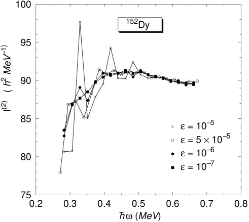
Figure 1: The dynamical moment of inertia for different accuracies in the LN calculations. $\varepsilon$ is given in MeV.

3.1 The Yrast band of ¹⁶⁴Er

The first example we would like to show is the Yrast line of the nucleus ¹⁶⁴Er. It is well known that this nucleus presents a backbending at around spin $16\hbar$, due to the alignment of a neutron pair. This alignment causing a quenching of the neutron pairing correlations at high spins. This nucleus is therefore a very stringent test for the LN prescription and the SCK2 approximation.

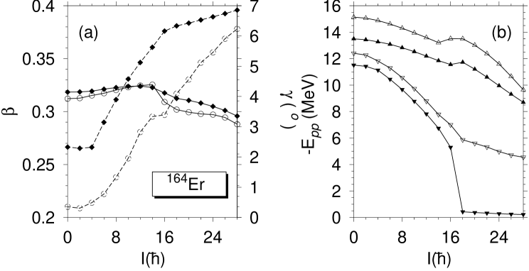
Figure 2: Comparison of LN and SCK2 results versus angular momentum for ${}^{164}Er$ along the Yrast band. (a) $\beta$ (full lines, left hand side scale) and $\gamma$ (dashed lines, right hand side scale) deformation parameters. The full (open) symbols correspond to the SCK2 (LN) approximation. (b) Pairing energies : full (empty) triangles correspond to protons in the SCK2 (LN) method. Inverted full (empty) triangles correspond to neutrons in the SCK2 (LN) method.

In Fig. (2a) we display the $(\beta,\gamma)$ deformation parameters of the rare earth nucleus ${}^{164}Er$ along the Yrast line in the LN and SCK2 methods. In both approximations, up to $I\approx 14\hbar$, we find a slight increase of the $\beta$ deformation parameter caused by the Coriolis antipairing effect. Above $I\approx 14\hbar$ and with increasing spin values we observe a decreasing of the $\beta$ deformation due to the antistretching effect. Though both approximations provide results close to each other the largest discrepancies appear for spin values above $I\approx 16\hbar$. The $\gamma$ deformation increases with the angular momentum in the LN and the SCK2 methods, the triaxiality of the SCK2 results being larger than the LN ones. Fig. (2b) displays the particle-particle correlation energy ($E_{pp}=\frac{1}{2}Tr(\Delta\kappa)$) for both methods along the Yrast band. The proton system behaves very similarly in both approaches, illustrating very clearly the rotation induced Coriolis antipairing effect, the SCK2 approach providing, though, somewhat smaller values than the LN one. The neutron system, however, behaves differently : while the results for $E_{pp}$ in the LN approach decrease from $-12$MeV at low spin to $-6$ MeV at spin value of $20\hbar$ and then change the slope to decrease more gentle, up to $-4$ MeV at spin $30\hbar$; the SCK2 values start at $-12$MeV at low spin decreasing to $-6$ MeV at a spin value of $16\hbar$, at this spin value they experiment a sharp drop to an almost unpaired regime.

To understand this behavior and to check the validity of the Kamlah expansion we display in Fig. (3) the values of the $h_{2}^{\tau,eff}$ parameter and the particle number fluctuation in both approaches along the Yrast band. In the LN approach the values of $h_{2}^{\pi,eff}$ and $h_{2}^{\nu,eff}$ remain small and constant at low and medium spins and increase slightly at high spin values. In the SCK2 approach, however, the $h_{2}^{\nu,eff}$ parameter is small and constant at low spins, increases smoothly up to a spin value of $16\hbar$ and then very suddenly rises to a large value, larger than one. On the right hand side of the figure we see how the particle number fluctuations in both approximations decrease more or less smoothly with the exception of the neutron number fluctuations in SCK2 which decrease rather sharply from about 6.5 to around 2 at spin value of $18\hbar$. Both, the large value of $h_{2}^{\nu,eff}$ and the smallness of $\langle(\Delta\hat{N})^{2}\rangle$ at high spin values are a clear indication of a breakdown of the Kamlah expansion to second order at the corresponding spin values. In the LN case we may observe a degradation of the expansion but one still remains in the correlated regime.

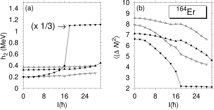
Figure 3: Comparison of LN and SCK2 results versus angular momentum for the Yrast band of ${}^{164}Er$. (a) $h_{2}^{eff}$ parameters : Full (empty) triangles correspond to protons in the SCK2 (LN) method. Inverted full (empty) triangles correspond to neutrons in the SCK2 (LN) method. (b) Same as panel (a), but for the standard deviations $\langle(\Delta\hat{N})^{2}\rangle$.

In Fig. 4, panel (a), we present the transition energies, $\Delta E_{I}=E(I)-E(I-2)$, versus the angular momentum, $I$, and in panel (b) the static moment of inertia ${\mathcal{I}}^{(1)}=(2I-1)/\Delta E_{I}$ versus the square of the angular frequency ($\omega(I)=\Delta E_{I}/2$), for ${}^{164}Er$ in the LN and the SCK2 approximate methods as well as the experimental data [17]. The LN results are in overall fair agreement with the experiment. Below the backbending region the pairing correlations are slightly over-valued. In the backbending region, as expected, the results are in poorer agreement with the experiment due to the well known fact that in the cranking approach the ground and aligned bands interact at fixed $\omega$ instead of fixed $I$. Above the backbending region the agreement with the experiment becomes again good. Concerning the SCK2 results, for the $I$-values below the backbending, where the Kamlah expansion is valid, one obtains a better agreement with the experiment that the LN approach. At $I=16\hbar$, where the Kamlah expansion breaks down, we get a huge change in the transition energy (not shown in the picture), much more pronounced than in the experiment. Beyond this spin value the SCK2 results are not as good as the LN ones. In panel (b) of Fig. 4, the backbending plot, ${\cal I}^{(1)}$ versus $(\hbar\omega)^{2}$, is displayed, here we can clearly see that in the region where the SCK2 method works the agreement with the experiment is better than in the LN approach. Outside this region the LN works again better. Of course, the Yrast line of the ¹⁶⁴Er nucleus is a very stringent case because of the backbending and we expect that the SCK2 approach will work in other situations.

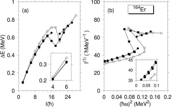
Figure 4: (a) Transition energies along the Yrast band of ¹⁶⁴Er as a function of the angular momentum. LN (open circles), SCK2 (full circles) and experimental data (full squares). (b) Comparison of the kinematic moments of inertia versus the square of the angular frequency. Same symbols as (a).

3.2 Superdeformed ground band of the nucleus ¹⁹⁰Hg.

Now we shall discuss the superdeformed ground band of the nucleus ¹⁹⁰Hg as an example of superdeformation in the $A\simeq 190$ region. Calculations in this region in the LN approach have been performed with the Skyrme force and a density dependent pairing force in [18] and with the relativistic mean field theory in [19]. In panel (a) of Fig. 5 we display the particle-particle correlation energy in the LN and SCK2 approaches. As before we obtain less correlations in the SCK2 approach than in the LN one, both approaches displaying the typical rotation induced Coriolis antipairing effect. For this nucleus, for all spin values, and in both approximations, the pair correlations are large enough to warrant the convergence of the Kamlah expansion.

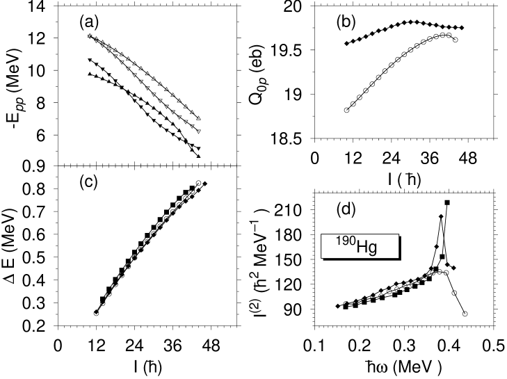
Figure 5: LN and SCK2 results for the superdeformed ground band of the nucleus ${}^{190}Hg$ mercury isotope. (a) Pairing energies versus angular momentum : Full (empty) triangles correspond to protons in the SCK2 (LN) method. Inverted full (empty) triangles correspond to neutrons in the SCK2 (LN) method. (b) Charge quadrupole moments versus angular momentum : open circles (full diamonds) represent the LN (SCK2) results. (c) Transition energies versus angular momentum : open circles (full diamonds) represent the LN (SCK2) results. The experimental values are depicted by full squares. (d) Dynamic Moment of inertia ${\mathcal{I}}^{(2)}$ versus the angular frequency $\hbar\omega$ : same symbols as in panel (c).

In panel (b) the charge quadrupole moments are shown. At low spin values the SCK2 values are somewhat larger than the LN ones, due in part to the fact that the latter ones are more pair-correlated, while at higher spins they get closer. Both predictions are slightly larger than the experimental value of $17.7^{+1}_{-1.2}$ eb [20]. The transition energies $\Delta E_{I}$ are shown in panel (c), at low and medium spins both approaches are very close to each other and in good agreement with the experimental data [21]. At high spins, though the overall agreement with the experimental data is better in the LN approach, a careful look reveals that the down bending of the experimental two last points is not provided in this approach. The SCK2 method, however, describes this feature. This behavior can be more clearly seen in the plot of the second moment of inertia, ${\cal I}^{(2)}=4/(\Delta E_{I}-\Delta E_{I-2})$, in panel (d). Here we observe that the theoretical predictions closely follow the experimental data up to $\hbar\omega\simeq 0.35$ MeV. From this point on the experimental data display an upbending that the LN results do not follow, the SCK2 results, however, clearly show the same behavior as in the experiment. We can understand the reason for this upbending looking at Fig. 6, where the quasiparticle energies versus the angular frequency for the relevant channels in the LN and SCK2 approaches are plotted. The main difference between both approaches is that in the LN case the splitting of the signature partner levels $\nu[761]3/2$ and $\pi[642]5/2$, close to the Fermi surface, is larger than in the SCK2 case. The signature partner levels $\nu[761]3/2$ align at $\hbar\omega\simeq 0.35MeV$ in the SCK2 case, in the LN approach there is a delay in the alignment of the negative signature level with respect to the positive one. We have checked the parameter $h_{2}^{eff}$ and the fluctuations $\langle(\Delta\hat{N})^{2}\rangle$ and the Kamlah expansion does not break down in this case.

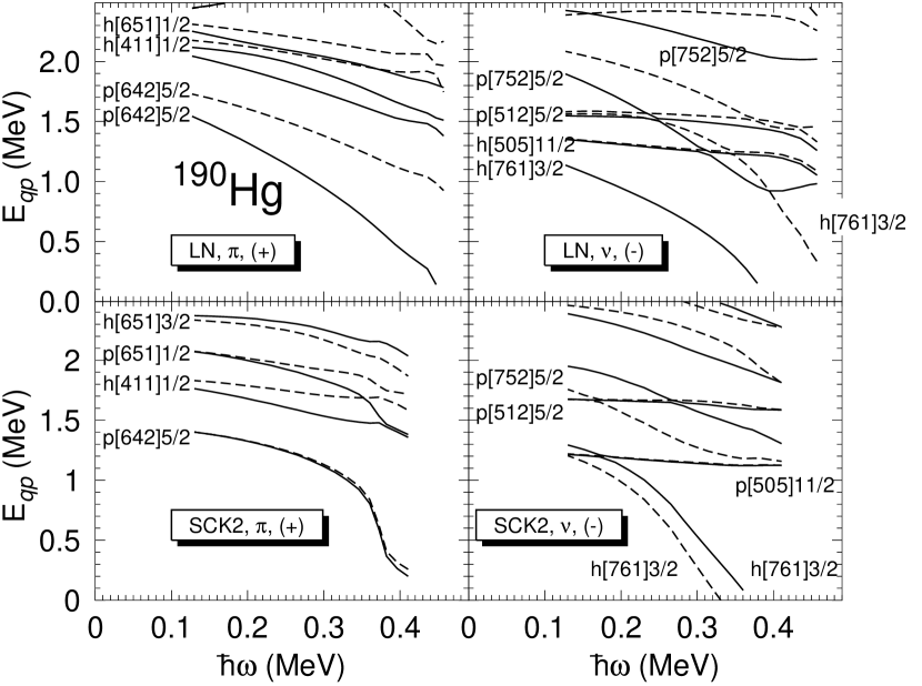
Figure 6: Quasiparticle energies versus the angular frequency $\hbar\omega$ for the SD ground state band of ${}^{190}Hg$. Only the positive parity proton and negative parity neutron orbitals are shown. Orbitals of positive (negative) signature are represented by solid (dashed) lines.

3.3 Superdeformed ground band of the nucleus ¹⁵²Dy

Next we shall turn to discuss an example of a SD nucleus in the $A\sim 150$ region, namely ¹⁵²Dy. Calculations in this region in the LN approach have been performed with the Skyrme force and a density dependent pairing force in [22]. As before, we have calculated the ground superdeformed band in the LN and in the SCK2 approaches. In Fig. 7a we display the particle-particle correlation energy along this band. The behavior of $E_{pp}$ with increasing angular momentum is similar to the ones in the already discussed nuclei. We have to notice, however, that at high angular momentum the correlations are small and that this nucleus is, so far, the only case, in our calculations, where the proton pair correlations are larger in the SCK2 approach than in the LN one. In panel (b) the charge quadrupole moment is depicted, again the largest difference between both approximations takes place at low spins where the pair correlations differ at most, at high spins they get closer. The SCK2 moments are rather constant with spin, as one would expect for a superdeformed band, while the LN ones vary somewhat more. The LN results are in good agreement with the experimental data of $17.5\pm 0.2$ eb [23] whereas the SCK2 are slightly higher. In panel (c) the transition energies are shown, though both approaches provide good results as compared with the experimental data [24] the SCK2 ones are slightly better. Finally in panel (d) the second moment of inertia is plotted versus the angular frequency. At medium and high spins the LN approach provides constant values of ${\cal I}^{(2)}$ as in the experiment though somewhat larger. The LN results at low spins are too low as compared to the experiment.

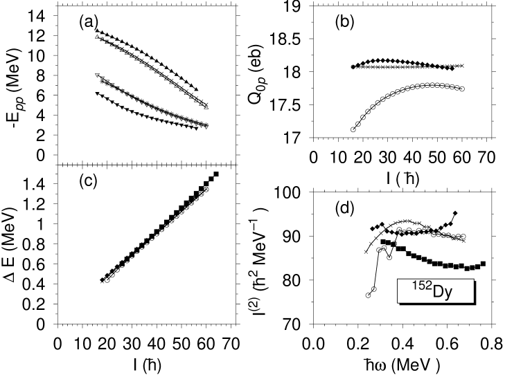
Figure 7: Same as Fig. 4 but for the nucleus ¹⁵²Dy. The additional symbols are explained in the text.

At low and medium angular frequencies the ${\cal I}^{(2)}$ values in the SCK2 approximation are rather constant with spin, though they are somewhat larger than the experimental data. At low spins the SCK2 approximation, however, is in better agreement with the experiment than the LN approach. At high angular frequency the SCK2 results increase too fast. Concerning the convergence of the Kamlah expansion, in the SCK2 at spin values above $56\hbar$ we obtain large values of $h_{2}$ and very small $\langle(\Delta\hat{N})^{2}\rangle$ indicating that the expansion breaks down. As a matter of fact, the $h_{2}$ values of the last points displayed in the figure have $h_{2}$ values somewhat larger than one. In the LN case the $h_{2}$ values are always small (around $0.5$) and rather constant.

The most striking difference between the LN and the SCK2 results in both SD nuclei studied is the behavior of the quadrupole moment at low spins. The SCK2 results look more reasonable because they keep rather constant quadrupole moment with the spin as one would expect from a superdeformed object. It seems, therefore, that the LN values at low spins are less confident. Others, not well understood, facts of the LN approach are the slow convergence at low spins discussed in section 3 and the behavior of the second moment of inertia at low spins in ¹⁵²Dy. In order to investigate these facts we have performed quadrupole moment constrained LN (LNC) calculations. We have calculated the SD band with the additional constraint that each state of the band has a quadrupole moment equal to a constant value close to the SCK2 at high angular momentum. The results are depicted in Fig. 7, all results are represented by crosses with the exception of the neutron particle-particle correlation energy in panel (a) that is represented by asterisks. In this panel we observe that the results of the LN constrained calculations for $E_{pp}$ are more or less the same as the unconstrained ones. In panel (b) the constant constrained quadrupole moment is shown, this value is closer to the unconstrained LN ones at high spins, we expect, therefore, larger differences between both approaches at small rather than at large angular momentum. In panel (c) we see that the LNC transition energies and the LN ones do coincide at high spins, and that at small spins the LNC ones are closer to the SCK2 and to the experiment than the LN ones. In panel (d), lastly, we observe that the behavior of the second moment of inertia is more reasonable at low spins in the LNC approach that in the LN one.

Figure 8: (a) Static moment of inertia versus the square of the angular frequency for the SD ground band of ¹⁵²Dy. (b) Energy differences between the LN (LNC) and the SCK2 approaches.

To gain more insight in the different approaches we have represented in Fig. (8a) the kinematical moment of inertia ${\cal I}^{(1)}$ versus the square of the angular frequency. The experimental results are rather constant at large angular momenta and they slightly decrease at small angular momentum. The LN results behave properly, though a little too large, at high angular momentum. At small angular momentum they have an unexpected behavior. The SCK2 results at small angular momentum behave well and at high $I$ converge to the LN results. The LNC calculations on the other hand give the right behavior at small angular momentum. In Fig. (8b) we finally present the energy differences between the LN approaches and the SCK2. Obviously the SCK2 approach provides the deepest energy. Concerning the LN and the LNC values, it is interesting to realize that the LNC energies are always deeper or equal to the LN ones. This is not a situation to wonder because the LN approach is not variational and there is no reason, therefore, to expect that by changing some expectation value we must go up, necessarily, in the energy.

This example illustrates clearly that the LN approach, occasionally, may fail to find the right minimum because it is not a variational method. This failure being, probably, the cause of the slow convergence rate found in some cases. It is important to notice that this happens in the strong pairing regime, this behavior was not observed in earlier investigations [5, 9] probably because the considered model was too simplistic.

4 Conclusions

In conclusion, for the first time, we have performed selfconsistent calculations of approximate particle number projection within the Kamlah expansion to second order with density dependent forces (Gogny force). In particular, we have reported calculations for the yrast band of the well-deformed rare earth nucleus ${}^{164}Er$, and the superdeformed ground bands of nuclei ${}^{190}Hg$ and ${}^{152}Dy$. In all cases, comparisons have been made with previous LN calculations and with available experimental data. As a result we find that the Kamlah expansion to second order may break down in situations of weak pairing when the minimization equations are solved fully variational (SCK2). In the Lipkin-Nogami approach, however, this has never happened in the cases analyzed so far. In the regimes where the expansion is valid, the fully variational approach provides results closer to the experiment than the non-variational (LN) ones. On the other hand, the LN approach has the drawback of the slow convergence in the iteration process and of not finding the right minimum in some isolated cases in the strong pairing regime, causing a low convergence rate in the iteration process.

This work was supported in part by DGICyT, Spain under Project PB97–0023.

References

- [1] H. J. Lipkin, Ann. Phys. (N.Y.) 12, 425 (1960).
- [2] Y. Nogami, Phys. Rev. B134, 313 (1964); Y. Nogami and I.J. Zucker, Nucl. Phys. 60, 203 (1964).
- [3] J. F. Goodfellow and Y. Nogami, Can. J. Phys. 44, 1321 (1966).
- [4] P. Quentin, N. Redon, J. Meyer and M. Meyer, Phys. Rev. C41, 41 (1990).
- [5] D. C. Zheng, D.W.L. Sprung and H. Flocard, Phys. Rev. C46, 1335 (1992).
- [6] A.Valor, J.L.Egido, L.M. Robledo, Phys. Rev. C53, (1996), 172.
- [7] A. Valor, J.L. Egido, L.M. Robledo, Nucl. Phys. A, in press.
- [8] A. Kamlah, Z. Phys. 216, 52 (1968).
- [9] J. Dobaczewski and W. Nazarewicz, Phys. Rev. C47, 2418 (1993).
- [10] D. Gogny, Nuclear Selfconsistent fields. Eds. G. Ripka and M. Porneuf (North Holland 1975).
- [11] P. Ring and P. Schuck, The Nuclear Many Body Problem (1980), Springer–Verlag Edt. Berlin.
- [12] A. Valor, Ph. D. Thesis, Universidad Autónoma de Madrid, 1996, unpublished.
- [13] A. Valor, J.L. Egido, L.M. Robledo, Phys. Lett. B392 , (1997), 249-254 .
- [14] J.F. Berger, M. Girod and D. Gogny, Nucl. Phys. A428, 23c (1984).
- [15] J.F. Berger, M. Girod and D. Gogny, Comp. Phys. Comm. 63(1991) 365-374
- [16] J.L. Egido, J. Lessing, V. Martin and L.M. Robledo, Nucl. Phys. A594 (1995)70-86
- [17] S.W. Yates et al. Phys. Rev. C21, 2366 (1980).
- [18] J. Terasaki, P.-H. Heenen, P. Bonche, J. Dobaczewski and H. Flocard, Nucl. Phys. A593 (1995) 1-20
- [19] A.V. Afanasjev, J. König, P. Ring, Phys. Rev. C60, in press.
- [20] H. Amro et al. Phys. Lett B413 (1997) 15
- [21] B. Crowell et al., Phys. Rev C51(1995) R1599
- [22] P. Bonche, H. Flocard and P.-H. Heenen, Nucl. Phys. A598 (1996) 169
- [23] H. Savajols et al., Phys. Rev. Lett. 76 (1996) 4480
- [24] D. Nisius at al., Phys. Lett. 392B (1997) 18