Approximate particle number projection with density dependent forces: Superdeformed bands in the A=150 and A=190 regions

Abstract

We derive the equations for approximate particle number projection based on mean field wave functions with finite range density dependent forces. As an application ground bands of even-A superdeformed nuclei in the $A=150$ and $A=190$ regions are calculated with the Gogny force. We discuss nuclear properties such as quadrupole moments, moments of inertia and quasiparticle spectra, among others, as a function of the angular momentum. We obtain a good overall description.

1 Introduction

Understanding pairing correlations has been and still remains a challenge for nuclear physicists. Several decades ago it was thought that pairing correlations will only affect a few nuclei and the properties of a few observables at low energy and small angular momentum; mainly the level density of odd nuclei as compared with the even ones, the energy of the two quasiparticle states and the moments of inertia of rotational nuclei. Such simplistic view has changed over the years in such a way that nowadays we expect pairing correlations playing a major role in many nuclear phenomena. To mention a few recent examples let us remember the important role of pairing correlations in halo nuclei, in $N=Z$ systems and in the understanding of the second moment of inertia in superdeformed nuclei.

In spite of all that the theoretical understanding of the pairing force is rather limited. The recognition of this fact has motivated in the last years a proliferation of approximate methods (Lipkin-Nogami, Kamlah at second order and exact particle number projection) and new pairing forces (density dependent, surface and volume pairing).

Within the mean field approaches the most successful calculations, aiming at describing low energy nuclear structure phenomena have been performed with density dependent forces. The most popular, because of its simplicity, is the Skyrme force. Most of the calculations have been performed with the SkM^∗ parameterization [1, 2]. The main disadvantage of the Skyrme interaction is that realistic pairing matrix elements cannot be extracted from the force, and therefore the pairing interaction (normally a monopole pairing term) has to be added by hand. Recently, other alternative forms of the pairing interaction, like density dependent pairing have been explored in connection with the Skyrme interaction [3, 4, 5]. Theories beyond mean field with simple pairing forces have been also developed [6]. Pairing properties, on the other hand, are very important in the description of high spin properties. Since the pioneer work of Mottelson and Valatin [8] many papers and experiments have been devoted to this topic. This is why the investigation of high spin states with a realistic force that is able to treat the short range correlations properly is most desirable. The Gogny force [9] is well known for providing, with the same set of parameters, a good description of many nuclear properties at low spins over the nuclide chart as, for example, ground state energies, odd-even mass differences, electron scattering data [10], fission barriers [11], etc. The main ingredients of the force are the phenomenological density dependent term which was introduced to simulate the effect of a G-matrix interaction and the finite range of the force which provides the pairing matrix elements from the force itself. In recent calculations the Gogny force has been applied to high spin problems at normal deformations [12] and to superdeformed shapes [13, 14].

In these calculations the cranked HFB approximation (CHFB) was used. The angular momentum and number of particles of the system were determined by the corresponding constraints on the wave function. It turned out [12], however, that in spite of the finite range of the force, the condition of holding the particle number to be right on the average was not enough and a superfluid normalfluid sharp phase transition was found, contrary to what one would expect for a finite system. To remedy this problem, in [15] we have formulated the Lipkin-Nogami method for density dependent forces, the so-called CHFB Lipkin-Nogami approximation(CHFBLN). When this formalism was applied the sharp phase transition was washed out, the results of the calculations being in much better agreement with the experiment.

The purpose of this paper is to report on calculations in the $A=190$ and $A=150$ regions within the CHFB and CHFBLN approximations and the Gogny force. In section 2.1 we first derive the Lipkin-Nogami approximation from the Kamlah expansion to second order. In sect. 2.2 we extend this formalism to density dependent forces obtaining an extra contribution due to the rearrangement term. In sect. 3.1 we discuss results for the $A=190$ region, namely for the ^190-192-194Hg and ¹⁹⁴Pb, and in sect. 3.2 the $A=150$ region, taking as examples the ¹⁵²Dy and ¹⁵⁰Gd nuclei. We conclude the paper with conclusions and some appendixes.

2 Projected Mean Field Theories

Mean field theories (MFT) are based on the assumption of a product wave function; they constitute the basic (and in most cases the only one feasible) approximation to a many body system. The success of MFT is based on the concept of spontaneous symmetry breaking. By this mechanism the Hilbert space is considerably enlarged and many correlations can be taken into account. Obviously, the corresponding wave functions have to be considered as “intrinsic” wave functions. The most sophisticated mean field theory is the HFB approximation, in which the intrinsic wave function $|\Phi\rangle$ is defined as the non-trivial vacuum to the quasi-particle annihilation operators

$$\alpha_{\mu}=\sum_{i}U_{i\mu}^{*}c_{i}+V_{i\mu}^{*}c_{i}^{+},$$ (1)

where $\left\{c_{i},c_{i}^{+}\right\}$ is the set of single particle creation and annihilation operators in terms of which the quasi-particle operators are expanded, $U$ and $V$ are the so-called Bogoliubov wave functions. Product wave functions, $|\Phi\rangle$, of quasiparticles $\alpha_{\mu}$, in general, are neither eigenfunction of the angular momentum nor of the particle number operator. For heavy, well deformed nuclei, the usual approach of demanding that, at least, the expectation values of the angular momentum and the particle number operators take the right value, is a good approximation for the angular momentum but not for the particle number. This has to do with the number of nucleons participating in the breaking of the associated symmetry [17].

The ideal treatment of pairing correlations in nuclei is particle number projection (PNP) before the variation [17]. At high spin this theory is rather complicated to implement and up to now it has only been applied to separable forces [18]. On the other hand, the semi-classical recipe of solving the mean field equations with a constraint on the corresponding symmetry operator can be derived as the first order approach to a full quantum-mechanical expansion (the Kamlah expansion [19]) of the projected quantities. The second order in this expansion takes into account the particle number fluctuations and might cure some of the deficiencies of the first order approximation. However, full selfconsistent calculations up to second order are rather cumbersome and just simple model calculations have been carried out up to now [20]. Most second order calculations have been done using the Lipkin-Nogami (LN) recipe, which was originally proposed in Refs. [21, 22, 23]. Recently, the LN method has been applied to study superdeformed nuclei at high spins adding a monopole pairing interaction to the Woods-Saxon plus Strutinsky approximation [24], and to the Skyrme force [25].

The usual derivation of the LN method is not valid for density dependent forces because the dependence in density is not taken explicitly into account. In refs.[15, 16] the LN approach was generalized to properly deal with this situation. The derivation is based in the Kamlah expansion for the particle number projected energy. In the new formulation additional terms arise in the equations determining the parameters of the theory. To introduce the approximation and the corresponding notation we make in the following a short derivation of it.

2.1 First and second order approximation to exact particle number projection : Derivation for non-density dependent forces

The LN method can be derived using different arguments. As the usual ways of deriving the LN method are not well suited for a generalization to the case of density dependent forces, in this section we shall derive the equations for non-density dependent forces using the Kamlah expansion. This derivation can be easily extended to the density dependent case, see sec. 2.2.

Let $|\Phi\rangle$ be a product wave function of the Hartree-Fock-Bogoliubov type, i.e. a particle number symmetry violating wave function. We can generate an eigenstate of the particle number, $|\Psi_{N}\rangle$, by the projection technique [17]

$$|\Psi_{N}\rangle=\hat{P}^{N}|\Phi\rangle=\frac{1}{2\pi}\int_{0}^{2\pi}d\phi e^{i(\hat{N}-N)\phi}|\Phi\rangle.$$ (2)

The particle number projected energy is given by

$$E^{N}_{proj}=\frac{\langle\Psi_{N}|\hat{H}|\Psi_{N}\rangle}{\langle\Psi_{N}|\Psi_{N}\rangle}=\frac{\int_{0}^{2\pi}d\phi e^{-i\phi N}\langle\Phi|\hat{H}e^{i\phi\hat{N}}|\Phi\rangle}{\int_{0}^{2\pi}d\phi e^{-i\phi N}\langle\Phi|e^{i\phi\hat{N}}|\Phi\rangle}=\frac{\int_{0}^{2\pi}d\phi e^{-i\phi N}h(\phi)}{\int_{0}^{2\pi}d\phi e^{-i\phi N}n(\phi)},$$ (3)

where we have introduced the Hamiltonian and norm overlaps

$$h(\phi)=\langle\Phi|\hat{H}e^{i\phi\hat{N}}|\Phi\rangle,\;\;\;\;\;\;\;\;n(\phi)=\langle\Phi|e^{i\phi\hat{N}}|\Phi\rangle.$$ (4)

In the case of large particle numbers and strong deformations in the gauge space associated to $\hat{N}$, one expects the $h(\phi)$ and $n(\phi)$ overlaps to be peaked at $\phi=0$ and to be very small elsewhere in such a way that the quotient $h(\phi)/n(\phi)$ behaves smoothly. In this case one can make an expansion of $h(\phi)$ in terms of $n(\phi)$ in the following way [19]

$$h(\phi)=\sum_{m=0}^{M}h_{m}{\hat{\cal{N}}}^{m}n(\phi),$$ (5)

where we have introduced the Kamlah operator

$$\hat{\cal{N}}=\frac{1}{i}\frac{\partial}{\partial{\phi}}-\langle\Phi|\hat{N}|\Phi\rangle,$$ (6)

which is a representation of the particle number operator in the space of the parameter $\phi$. $M$ represents the order of the expansion, for $M\rightarrow\infty$ eq. (5) is exact. For large symmetry breaking systems and large particle number one expects convergence with a few terms. The expansion coefficients $h_{m}$ are determined by applying the operators $1,\hat{\cal{N}},...,\hat{\cal{N}}^{M}$ on eq. (5) and taking the limit $\phi\rightarrow 0$, one obtains

$$\langle\Phi|\hat{H}(\Delta{\hat{N}})^{n}|\Phi\rangle=\sum_{m=0}^{M}h_{m}\langle\Phi|(\Delta{\hat{N}})^{m+n}|\Phi\rangle$$ (7)

with $\Delta\hat{N}=\hat{N}-\langle\Phi|\hat{N}|\Phi\rangle$ and $n=0,\dots,M$. The previous equality provides an $M+1$ equations system, $h_{0},h_{1},\dots,h_{M}$ being the unknowns. From now on we will use the shorthand notation $\langle\hat{A}\rangle\equiv\langle\Phi|\hat{A}|\Phi\rangle$. Substitution of eq. (5) in eq. (3) provides the projected energy to order $M$

$$E^{M}_{proj}=\sum_{m=0}^{M}h_{m}(N-\langle\hat{N}\rangle)^{m}$$ (8)

This expression tell us that to determine the wave function $|\Phi\rangle$, in an approximate (to order $M$) projection before the variation, we have to minimize eq. (8). To first order, i.e. $M=1$, one obtains

$$E^{(1)}_{proj}\;=\;h_{0}\;\;+\;\;h_{1}\;(N-\langle\hat{N}\rangle),$$ (9)

with

$$h_{0}=\langle\hat{H}\rangle,\;\;\;\;\;\;\;\;h_{1}=\frac{\langle H\Delta N\rangle}{\langle(\Delta N)^{2}\rangle}.$$ (10)

In this case to minimize the approximate projected energy, we have to solve the HFB equations with the constraint $\langle\hat{N}\rangle=N$, i.e. the old BCS recipe. This approximation is expected to be good for very strong violating wave functions. In atomic nuclei where only a few pairs participate in the pairing correlations, we do not expect the first order approximation to be a good one.

For $M=2$ one obtains the following equations system for the coefficients $h_{0},h_{1}$ and $h_{2}$

$$\left\{\begin{array}[]{llll}\langle\hat{H}\rangle&=\;h_{0}&\;+\;0&+\;h_{2}\langle(\Delta\hat{N})^{2}\rangle\\ \langle\hat{H}\Delta{\hat{N}}\rangle&=\;0&\;+\;h_{1}\langle(\Delta\hat{N})^{2}\rangle&\;+\;h_{2}\langle(\Delta\hat{N})^{3}\rangle\\ \langle\hat{H}(\Delta{\hat{N}})^{2}\rangle&=\;h_{0}\langle(\Delta\hat{N})^{2}\rangle&\;+\;h_{1}\langle(\Delta\hat{N})^{3}\rangle&\;+\;h_{2}\langle(\Delta\hat{N})^{4}\rangle\end{array}\right.$$ (11)

the solution of this equations system provides

$$h_{0} = \langle\hat{H}\rangle-h_{2}\langle(\Delta\hat{N})^{2}\rangle$$ (12)

$$h_{1} = \frac{\langle\hat{H}\Delta\hat{N}\rangle-h_{2}\;\langle(\Delta\hat{N})^{3}\rangle}{\langle(\Delta\hat{N})^{2}\rangle}$$ (13)

$$h_{2} = \frac{\langle(\hat{H}-\langle\hat{H}\rangle)(\Delta\hat{N})^{2}\rangle-\langle\hat{H}\Delta\hat{N}\rangle\langle(\Delta\hat{N})^{3}\rangle/\langle(\Delta\hat{N})^{2}\rangle}{\langle(\Delta\hat{N})^{4}\rangle-\langle(\Delta\hat{N})^{2}\rangle^{2}-\langle(\Delta\hat{N})^{3}\rangle^{2}/\langle(\Delta\hat{N})^{2}\rangle}$$ (14)

The projected energy to second order is given by

$$E^{(2)}_{proj}\;=\;\langle\hat{H}\rangle\;\;-\;\;h_{2}\langle(\Delta\hat{N})^{2}\rangle\;\;+\;\;h_{1}\;(N-\langle\hat{N}\rangle)\;\;+\;\;h_{2}\;(N-\langle\hat{N}\rangle)^{2}$$ (15)

In a full variation after projection method one should vary $E^{(2)}_{proj}$ and compute cumbersome expressions like $\frac{\delta h_{2}}{\delta\Phi}$. In the Lipkin-Nogami prescription, however, the coefficient $h_{2}$ is held constant during the variation. As a result the variational equation is much simpler, one gets

$$\frac{\delta}{\delta\Phi}\langle\hat{H}\rangle-h_{1}\frac{\delta}{\delta\Phi}\langle\hat{N}\rangle+(N-\langle\hat{N}\rangle)\frac{\delta h_{1}}{\delta\Phi}-2h_{2}(N-\langle\hat{N}\rangle)\frac{\delta}{\delta\Phi}\langle\hat{N}\rangle-h_{2}\frac{\delta}{\delta\Phi}\langle(\Delta\hat{N})^{2}\rangle=0.$$ (16)

It is obvious that the solution to this equation is given by

$$\frac{\delta}{\delta\Phi}\langle\hat{H}-h_{2}(\Delta\hat{N})^{2}\rangle-\lambda\frac{\delta}{\delta\Phi}\langle\hat{N}\rangle=0,$$ (17)

with $\lambda$ determined by the constraint

$$\langle\hat{N}\rangle=N,$$ (18)

provided the condition $\lambda=h_{1}$ is accomplished. This can be easily realized noticing that eq. (17) must hold for any variation $|\delta\Phi\rangle$, in particular, we can choose $|\delta\Phi\rangle=\Delta\hat{N}|\Phi\rangle$. Substitution of this specific variation in eq. (17) provides

$$\langle\hat{H}\Delta\hat{N}\rangle-\lambda\langle(\Delta\hat{N})^{2}\rangle-h_{2}\langle(\Delta\hat{N})^{3}\rangle=0$$ (19)

comparison with eq. (13) shows that $\lambda=h_{1}$.

We have formulated the approximation for one class of nucleons (i.e. protons or neutrons), in practical cases one has to do it simultaneously for protons and neutrons but it is easy to show that for $M=2$ there is no coupling between protons and neutrons. The energy to be minimized is

$$E^{(2)}_{proj}=\langle\hat{H}\rangle-h^{\rm{Z}}_{2}\langle(\Delta\hat{\rm{Z}})^{2}\rangle-h^{\rm{N}}_{2}\langle(\Delta\hat{\rm{N}})^{2}\rangle,$$ (20)

with the constraints $\langle\hat{\rm{Z}}\rangle=\rm{Z}$ and $\langle\hat{\rm{N}}\rangle=\rm{N}$. In these expressions $\rm{Z}$ stands for protons and $\rm{N}$ for neutrons, $h^{\rm{Z}}_{2}$ is given by eq. (14), where the number operator in this equations should be substituted by the proton number operator, $h^{\rm{N}}_{2}$ is defined correspondingly. In the same manner if there are additional constraints, for example the angular momentum, one just has to substitute $\hat{H}$ by $\hat{H^{\prime}}=\hat{H}-\omega\hat{J_{x}}$ in all equations above with $\omega$ chosen in such a way that the constraint $\langle\hat{J_{x}}\rangle=[I(I+1)-\langle\hat{J_{z}}^{2}\rangle]^{1/2}$ is accomplished.

2.2 First and second order approximation to exact particle number projection: Derivation for density dependent forces

Now we would like to generalize the formulae of the former section to density dependent forces, like the Gogny force [9, 10, 11]

$$v_{12}(\rho) = \sum_{i=1,2}e^{-(\vec{r}_{1}-\vec{r}_{2})^{2}/\mu_{i}}\left(W_{i}+B_{i}P_{\sigma}-H_{i}P_{\tau}-M_{i}P_{\sigma}P_{\tau}\right)$$ (21)

$$+ iW_{LS}(\vec{\nabla}_{12}\delta(\vec{r}_{1}-\vec{r}_{2})\wedge\vec{\nabla}_{12})(\vec{\sigma}_{1}+\vec{\sigma}_{2})$$

$$+ t_{3}(1+P_{\sigma}x_{0})\delta(\vec{r}_{1}-\vec{r}_{2})\rho^{1/3}(\frac{\vec{r}_{1}+\vec{r}_{2}}{2}),$$

where the dependence on the wave function $|\Phi\rangle$, through the density $\rho(\vec{r})=\langle\Phi|c^{\dagger}(\vec{r})c(\vec{r})|\Phi\rangle$, adds some peculiarities.

Density dependent forces do not exhibit, in general, the same properties as the bare two-nucleon force. Let $|\Phi\rangle$ be a $\hat{S}$-symmetry breaking wave function and $v_{12}(\rho)$ the corresponding interaction. It is obvious that

$$\hat{S}v_{12}(\rho)\hat{S}^{-1}=v_{12}(\hat{S}\rho\hat{S}^{-1}).$$ (22)

That means, the two-body interaction in a $\hat{S}$-rotated system is the same as the interaction calculated with the rotated density. Eq. (22) is valid for any symmetry $\hat{S}$, in the particular case of symmetries with no dependence on the spatial coordinate $\vec{r}$, for example the particle number, it also holds

$$\hat{S}v_{12}(\rho)\hat{S}^{-1}=v_{12}(\hat{S}\rho\hat{S}^{-1})\equiv v_{12}(\rho),$$ (23)

i.e. the $v_{12}(\rho)$ interaction and the generators of the symmetry $\hat{S}$ do commute. In particular, for the particle number, in which we are interested here, $v_{12}(\rho)$ satisfies the same properties as the bare force.

In the context of plain mean field theories there is no ambiguity left concerning the density dependence of the hamiltonian. In theories beyond mean field, for example the Generator Coordinate Method or projected theories, in evaluating the expectation value of the energy, appear matrix elements like $\langle\Phi|\hat{H}|\Phi^{\prime}\rangle$, or in the case of PNP, the overlap $\langle\Phi|\hat{H}e^{i\phi\hat{N}}|\Phi\rangle$. Here a complication arises from the density dependent term of the hamiltonian because it is not obvious which density dependence should be taken in the potential (21). A Skyrme force with a linear dependence in the density can be cast as a three body force. For this particular case it can be shown that the density to be used in the hamiltonian in the evaluation of the matrix elements $\langle\Phi|\hat{H}|\Phi^{\prime}\rangle$ must be a non-diagonal density $\rho_{ND}(\vec{r})$ given by

$$\rho_{ND}(\vec{r})=\frac{\langle\Phi|c^{\dagger}(\vec{r})c(\vec{r})|\Phi^{\prime}\rangle}{\langle\Phi|\Phi^{\prime}\rangle}=\frac{\langle\Phi|\hat{\rho}(\vec{r})|\Phi^{\prime}\rangle}{\langle\Phi|\Phi^{\prime}\rangle},$$ (24)

where we have introduced the density operator $\hat{\rho}(\vec{r})=c^{+}(\vec{r})c(\vec{r})$. For the particular case of PNP, this density is given by $\rho_{ND}(\vec{r})=\langle\Phi|\hat{\rho}(\vec{r})e^{i\phi\hat{N}}|\Phi\rangle/\langle\Phi|e^{i\phi\hat{N}}|\Phi\rangle.$ Up to now, based on this result, the same prescription has been adopted for Skyrme forces with a non linear dependence in $\rho$ [26] as well as with the Gogny force [15]. This prescription is, however, not well founded. In the context of the LN approximation there have been two approaches to this problem. The first one [15], considers the energy as a functional of the densities (normal and abnormal) while the second one [16], is based on a many-body density dependence of the potential. These two methods are discussed in the following subsections.

2.2.1 Functionals of the density

In this section we shall derive the approximate particle number projection equations for potentials with a density dependence like eq. (21), using the prescription of appendix B to calculate the non-diagonal matrix elements of the hamiltonian. There the use of a density like (24) in the evaluation of non-diagonal matrix elements of any density dependent Hamiltonian was motivated.

The density dependence of the hamiltonian does not modify the projected energy of eq. (8) but only the coefficients $h_{m}$ of the expansion. The non-diagonal density causes a dependence on $\phi$ of the hamiltonian and eq. (5) looks like

$$\langle\Phi|\hat{H}(\phi)e^{i\phi\hat{N}}|\Phi\rangle=\sum_{m=0}^{M}h_{m}\hat{\cal{N}}^{m}\langle\Phi|e^{i\phi\hat{N}}|\Phi\rangle,$$ (25)

application of the operators $1,\hat{\cal{N}},...,\hat{\cal{N}}^{M}$ on eq. (25), in the limit $\phi\rightarrow 0$, now provides

$$\sum_{l=0}^{n}\left(\begin{array}[]{cc}n\\ l\\ \end{array}\right)\left.\left\langle(\Delta\hat{N})^{l}\;\frac{1}{i^{n-l}}\frac{\partial^{n-l}}{\partial\phi^{n-l}}\hat{H}(\phi)\right|_{\phi=0}\right\rangle=\sum_{m=0}^{M}h_{m}\langle(\Delta\hat{N})^{m+n}\rangle.$$ (26)

For $M=1$ the energy is given by eq. (9) and the coefficients $h_{0}$ and $h_{1}$ by

$$\langle\hat{H}\rangle = h_{0}$$

$$\left.\left\langle\frac{1}{i}\frac{\partial\hat{H}}{\partial\phi}\right|_{\phi=0}+\hat{H}\Delta\hat{N}\right\rangle = h_{1}\langle(\Delta\hat{N})^{2}\rangle,$$ (27)

the derivatives with respect to $\phi$ are calculated very easily, since

$${\left.\frac{1}{i}\frac{\partial\rho}{\partial\phi}\right|}_{\phi=0}={\left.\frac{1}{i}\frac{\partial}{\partial\phi}\frac{\langle\Phi|\hat{\rho}(\vec{r})e^{i\phi\hat{N}}|\Phi\rangle}{\langle\Phi|e^{i\phi\hat{N}}|\Phi\rangle}\right|}_{\phi=0}=\;\langle\hat{\rho}(\vec{r})\Delta\hat{N}\rangle$$ (28)

we obtain

$${\left.\frac{1}{i}\frac{\partial\hat{H}}{\partial\phi}\right|}_{\phi=0}=\frac{1}{i}\frac{\partial\hat{H}}{\partial\rho}{\left.\frac{\partial\rho}{\partial\phi}\right|}_{\phi=0}=\;\langle\hat{\rho}\Delta\hat{N}\rangle\frac{\partial\hat{H}}{\partial\rho}.$$ (29)

Substitution in eq. (27), provides the coefficient $h_{1}$

$$h_{1}=\frac{\langle\Phi|\hat{H}\Delta\hat{N}|\Phi\rangle}{\langle\Phi|(\Delta\hat{N})^{2}|\Phi\rangle}+\left\langle\Phi\left|\frac{\partial H(\rho)}{\partial\rho(r)}\frac{\langle\Phi|\hat{\rho}\Delta\hat{N}|\Phi\rangle}{\langle\Phi|(\Delta\hat{N})^{2}|\Phi\rangle}\right|\Phi\right\rangle.$$ (30)

This expression for $h_{1}$ is exactly the same obtained in the selfconsistent HFB approximation, see eq. (61). It is interesting to notice that if we had used the density $\langle\Phi|\hat{\rho}(\vec{r}|\Phi\rangle$, instead of eq. (24), in the hamiltonian, the coefficient $h_{1}$ would be given by the first term of eq. (30), i.e. the rearrangement term would be missing, contrary to the HFB result, see appendix A.

For the $M=2$ case, we obtain

$$\langle\hat{H}\rangle = h_{0}\;\;+\;\;h_{2}\;\langle(\Delta\hat{N})^{2}\rangle$$

$$\left.\left\langle\frac{1}{i}\frac{\partial\hat{H}}{\partial\phi}\right|_{\phi=0}+\hat{H}\Delta\hat{N}\right\rangle = h_{1}\langle(\Delta\hat{N})^{2}\rangle+h_{2}\langle(\Delta\hat{N})^{3}\rangle$$ (31)

$$\left\langle\left.\left.\frac{1}{i^{2}}\frac{\partial^{2}\hat{H}}{\partial\phi^{2}}\right|_{\phi=0}+2\Delta\hat{N}\frac{1}{i}\frac{\partial\hat{H}}{\partial\phi}\right|_{\phi=0}\;+\;\hat{H}(\Delta\hat{N})^{2}\right\rangle = h_{0}\langle(\Delta\hat{N})^{2}\rangle+h_{1}\langle(\Delta\hat{N})^{3}\rangle+h_{2}\langle(\Delta\hat{N})^{4}\rangle.$$

The second derivative with respect to $\phi$ is given by

$${\left.\frac{1}{i^{2}}\frac{\partial^{2}\rho}{\partial\phi^{2}}\right|}_{\phi=0}=\;\langle\Delta\hat{\rho}(\Delta\hat{N})^{2}\rangle$$ (32)

and

$${\left.\frac{1}{i^{2}}\frac{\partial^{2}\hat{H}}{\partial\phi^{2}}\right|}_{\phi=0}=\langle\Delta\hat{\rho}\;\;\Delta\hat{N}\rangle^{2}\frac{\partial^{2}\hat{H}}{\partial\rho^{2}}+\langle\Delta\hat{\rho}\;\;(\Delta\hat{N})^{2}\rangle\frac{\partial\hat{H}}{\partial\rho}$$ (33)

From now on we proceed as in the non-density dependent case, i.e. we have to solve eq. ( 17 ) with the constraint (18) but with the coefficient $h_{2}$ given by the solution of equations system (31). It can be easily checked that the condition $\lambda=h_{1}$ also holds in this case.

2.2.2 Many-body density dependence of the Hamiltonian

In the former section we have interpreted the Gogny potential as a functional of the density and we have derived, under this assumption, the approximate particle number projected equations.

Another approach [16] to the same problem is to look at the expectation value $\langle\Psi_{N}|\hat{H}|\Psi_{N}\rangle$ of eq. (3) independently of the fact that $|\Psi_{N}\rangle$ is a many body wave function. In this case one could think of using the density $\langle\Psi_{N}|\hat{\rho}|\Psi_{N}\rangle/\langle\Psi_{N}|\Psi_{N}\rangle$ in the hamiltonian. This density, which we shall refer to as projected density is given by

$$\rho_{proj}(\vec{r})=\frac{\langle\Phi|\hat{P}^{N}\hat{\rho}(\vec{r})\hat{P}^{N}|\Phi\rangle}{\langle\Phi|P^{N}|\Phi\rangle}=\frac{\langle\Phi|\hat{\rho}(\vec{r})\hat{P}^{N}|\Phi\rangle}{\langle\Phi|P^{N}|\Phi\rangle},$$ (34)

and should be used in the Gogny force (21) in the calculation of the projected energy. We shall call $\hat{H}_{I}(\equiv\hat{H}(\rho_{proj}))$ the hamiltonian obtained with a dependence in the projected density. We would like to remark that the wave function $|\Phi\rangle$ in eq. (34) is a symmetry breaking one, i.e. it is not an eigenstate of $\hat{N}$. This guarantees the use of generalized Hamiltonians which are functionals of wave functions in the very large Hilbert space generated by symmetry breaking wave functions. Concerning the projection, we are now able to calculate the projected energy of eq. (3) and we can proceed along the same lines as in the derivation for non-density dependent forces, i.e. to use the Kamlah expansion up to order $M$. All expressions are the same, one just has to substitute $\hat{H}$ by $\hat{H}_{I}$ in all equations.

Calculation of the projected density may be quite involved. A way out is to approximate the projected density to be used in the hamiltonian. This can be done in the following way. Substitution of (2) in $\rho_{proj}(\vec{r})$ provides

$$\rho_{proj}(\vec{r})=\frac{\int_{0}^{2\pi}d\phi e^{-i\phi N}\langle\Phi|\hat{\rho}(\vec{r})e^{i\phi\hat{N}}|\Phi\rangle}{\int_{0}^{2\pi}d\phi e^{-i\phi N}\langle\Phi|e^{i\phi\hat{N}}|\Phi\rangle}=\frac{\int_{0}^{2\pi}d\phi e^{-i\phi N}\rho(r,\phi)}{\int_{0}^{2\pi}d\phi e^{-i\phi N}n(\phi)},$$ (35)

where we have introduced the overlap $\rho(\vec{r},\phi)=\langle\Phi|\hat{\rho}(\vec{r})e^{i\phi\hat{N}}|\Phi\rangle$. As with the Hamilton overlap, we may use the Kamlah expansion to approximate the projected density, i.e.

$$\rho(\vec{r},\phi)=\sum_{m=0,M}R_{m}(\vec{r})\hat{\cal{N}}^{m}n(\phi).$$ (36)

Substitution of eq. (36) in eq. (35) provides the projected nuclear density to order $M$

$$\rho^{(M)}_{proj}(\vec{r})=\sum_{m=0}^{M}R_{m}(\vec{r})(N-\langle\hat{N}\rangle)^{m}.$$ (37)

The expansion coefficients $R_{m}$ are determined applying the operators $1,\hat{\cal{N}},...,\hat{\cal{N}}^{M}$ on eq. (36). In the limit $\phi\rightarrow 0$, one obtains

$$\langle\Phi|\hat{\rho}(\vec{r})(\Delta{\hat{N}})^{n}|\Phi\rangle=\sum_{m=0}^{M}R_{m}(\vec{r})\langle\Phi|(\Delta{\hat{N}})^{m+n}|\Phi\rangle,$$ (38)

with $n=0,\dots,M$. To first order

$$\rho^{(1)}_{proj}(\vec{r})=R_{0}(\vec{r})+R_{1}(\vec{r})(N-\langle\hat{N}\rangle),$$ (39)

with $R_{0}=\langle\Phi|\hat{\rho}(\vec{r})|\Phi\rangle\equiv\rho(\vec{r})$, the HFB density, and

$$R_{1}(\vec{r})=\frac{\langle\hat{\rho}(\vec{r})\Delta\hat{N}\rangle}{\langle(\Delta\hat{N})^{2}\rangle}.$$ (40)

Assuming that $R_{1}(\vec{r})(N-\langle\hat{N}\rangle)$ is a small quantity as compared to $\rho(\vec{r})$ we can expand the density which appears in the Gogny force

$$[\rho^{(1)}_{proj}(r)]^{1/3} \approx\rho(\vec{r})^{1/3}\left[1+\frac{R_{1}(\vec{r})}{\rho(\vec{r})}(N-\langle\hat{N}\rangle)\right]^{1/3}$$ (41)

$$\approx \rho(\vec{r})^{1/3}+\frac{1}{3}\rho(\vec{r})^{-2/3}R_{1}(\vec{r})(N-\langle\hat{N}\rangle),$$

substitution of this expression in the Gogny hamiltonian with the projected density dependence, what we have called $\hat{H}_{I}$, provides

$$\hat{H}_{I}\equiv\hat{H}(\rho_{proj})\approx\hat{H}(\rho)+\frac{\partial\hat{H}}{\partial\rho}R_{1}(\vec{r})(N-\langle\hat{N}\rangle),$$ (42)

with $\hat{H}(\rho)$ the hamiltonian depending on the HFB density. The projected energy is given, up to $(N-\langle\hat{N}\rangle)$ order, by

$$E^{(1)}_{proj}=\langle\hat{H}_{I}\rangle+\frac{\langle H\Delta N\rangle}{\langle(\Delta N)^{2}\rangle}(N-\langle\hat{N}\rangle)=\langle\hat{H}\rangle+h_{1}^{\rm eff}(N-\langle\hat{N}\rangle)$$ (43)

with $h_{1}^{\rm eff}=\frac{\langle H\Delta N\rangle}{\langle(\Delta N)^{2}\rangle}+\langle\frac{\partial H}{\partial\rho}R_{1}(\vec{r})\rangle$. Minimization of this energy is equivalent to the minimization of $\langle\hat{H}\rangle-\lambda\langle\hat{N}\rangle$ subject to the constraint $\langle\hat{N}\rangle=N$ and $\lambda$ given by $h_{1}^{eff}$. Now $\lambda$ (or $h_{1}^{eff}$) includes the rearrangement term present in the HFB theory with density dependent forces. It is worth to point out that in this approach we obtain the same results as in the previous section , see eq. (30), and in the selfconsistent HFB approximation, see eq. (61).

To calculate the energy to second order one should also expand the density overlap to the same order. We obtain

$$\rho^{(2)}_{proj}(\vec{r})=\rho(\vec{r})+R_{1}(\vec{r})(N-\langle\hat{N}\rangle)+R_{2}(\vec{r})(N-\langle\hat{N}\rangle)^{2}-R_{2}(\vec{r})\langle(\Delta\hat{N})^{2}\rangle$$ (44)

with

$$R_{1}(\vec{r}) = \frac{\langle\hat{\rho}(\vec{r})\Delta\hat{N}\rangle-R_{2}(\vec{r})\;\langle(\Delta\hat{N})^{3}\rangle}{\langle(\Delta\hat{N})^{2}\rangle}$$ (45)

$$R_{2}(\vec{r}) = \frac{\langle(\hat{\rho}(\vec{r})-\langle\hat{\rho}(\vec{r})\rangle)(\Delta\hat{N})^{2}\rangle-\langle\hat{\rho}(\vec{r})\Delta\hat{N}\rangle\langle(\Delta\hat{N})^{3}\rangle/\langle(\Delta\hat{N})^{2}\rangle}{\langle(\Delta\hat{N})^{4}\rangle-\langle(\Delta\hat{N})^{2}\rangle^{2}-\langle(\Delta\hat{N})^{3}\rangle^{2}/\langle(\Delta\hat{N})^{2}\rangle}$$ (46)

As in eq. (41), we can make an expansion of the dependence of the hamiltonian on the projected density. After substitution of this expansion in the projected hamiltonian, we obtain

$$\hat{H}_{I}\approx\hat{H}(\rho)+\frac{\partial\hat{H}(\rho)}{\partial\rho(r)}\left[R_{1}(\vec{r})(N-\langle\hat{N}\rangle)+R_{2}(\vec{r})(N-\langle\hat{N}\rangle)^{2}-R_{2}(\vec{r})\langle(\Delta\hat{N})^{2}\rangle\right]$$ (47)

The projected energy for $M=2$ is given by

$$E^{(2)}_{proj}\;=\;\langle\hat{H}_{I}\rangle\;\;-\;\;{h}_{2}^{I}\langle(\Delta\hat{N})^{2}\rangle\;\;+\;\;{h}_{1}^{I}\;(N-\langle\hat{N}\rangle)\;\;+\;\;{h}_{2}^{I}\;(N-\langle\hat{N}\rangle)^{2}$$ (48)

with

$$h_{1}^{I} = \frac{\langle\hat{H}_{I}\Delta\hat{N}\rangle-h_{2}^{I}\;\langle(\Delta\hat{N})^{3}\rangle}{\langle(\Delta\hat{N})^{2}\rangle}$$ (49)

$$h_{2}^{I} = \frac{\langle(\hat{H}_{I}-\langle\hat{H}_{I}\rangle)(\Delta\hat{N})^{2}\rangle-\langle\hat{H}_{I}\Delta\hat{N}\rangle\langle(\Delta\hat{N})^{3}\rangle/\langle(\Delta\hat{N})^{2}\rangle}{\langle(\Delta\hat{N})^{4}\rangle-\langle(\Delta\hat{N})^{2}\rangle^{2}-\langle(\Delta\hat{N})^{3}\rangle^{2}/\langle(\Delta\hat{N})^{2}\rangle}.$$ (50)

The structure of eq. (48), is exactly the same as eq. (15) and so are the coefficients $h^{I}_{1},h^{I}_{2}$ and $h_{1},h_{2}$. From the discussion of eq. (15), it is obvious that the solution to this equation is given by

$$\frac{\delta}{\delta\Phi}\langle\hat{H_{I}}-h^{I}_{2}(\Delta\hat{N})^{2}\rangle-\lambda\frac{\delta}{\delta\Phi}\langle\hat{N}\rangle=0,$$ (51)

with $\lambda$ determined by the constraint

$$\langle\hat{N}\rangle=N,$$ (52)

provided the condition $\lambda=h^{I}_{1}$ is accomplished. Again, it can be checked that this is the case. Taking into account the particle number constraint we can write

$$\hat{H}_{I}\approx\hat{H}(\rho)-\frac{\partial\hat{H}(\rho)}{\partial\rho(r)}R_{2}(\vec{r})\langle(\Delta\hat{N})^{2}\rangle)$$

Substitution of $\hat{H}_{I}$ in $h^{I}_{2}$ provides

$$h_{2}^{I} = h_{2}-\frac{\langle(\frac{\partial\hat{H}}{\partial\rho(\vec{r})}R_{2}(\vec{r})-\langle\frac{\partial\hat{H}}{\partial\rho(\vec{r})}R_{2}(\vec{r})\rangle)(\Delta\hat{N})^{2}\rangle-\langle\frac{\partial\hat{H}}{\partial\rho(\vec{r})}R_{2}(\vec{r})\Delta\hat{N}\rangle\langle(\Delta\hat{N})^{3}\rangle/\langle(\Delta\hat{N})^{2}\rangle}{\langle(\Delta\hat{N})^{4}\rangle-\langle(\Delta\hat{N})^{2}\rangle^{2}-\langle(\Delta\hat{N})^{3}\rangle^{2}/\langle(\Delta\hat{N})^{2}\rangle}\langle(\Delta\hat{N})^{2}\rangle$$ (53)

$$= h_{2}+\delta h_{2}$$

with $h_{2}$ given by eq. (14). We have checked in some test cases that $\delta h_{2}$ is much smaller than $h_{2}$ and therefore in the following $\delta h_{2}$ is neglected. Assuming $\langle\hat{N}\rangle=N$, we can finally write the projected energy, eq. (48), to be minimized

$$E^{(2)}_{proj} \approx \langle\hat{H}\rangle-[\langle\frac{\partial\hat{H}}{\partial\rho(\vec{r})}R_{2}(\vec{r})\rangle+h_{2}]\langle(\Delta\hat{N})^{2}\rangle$$ (54)

$$= \langle\hat{H}\rangle-h_{2}^{eff}\langle(\Delta\hat{N})^{2}\rangle.$$

Where we have introduced the effective parameter $h_{2}^{eff}$

$$h_{2}^{eff}=\frac{(\langle\hat{\cal{H}}-\langle\hat{\cal{H}}\rangle)(\Delta\hat{N})^{2}\rangle-\langle\hat{\cal{H}}\Delta\hat{N}\rangle\langle(\Delta\hat{N})^{3}\rangle/\langle(\Delta\hat{N})^{2}\rangle}{\langle(\Delta\hat{N})^{4}\rangle-\langle(\Delta\hat{N})^{2}\rangle^{2}-\langle(\Delta\hat{N})^{3}\rangle^{2}/\langle(\Delta\hat{N})^{2}\rangle}$$ (55)

with

$$\hat{\mathcal{H}}=\hat{H}+\sum_{ij}\langle\frac{\partial\hat{H}}{\partial\rho(\vec{r})}f_{ij}(\vec{r})\rangle c^{+}_{i}c_{j}$$ (56)

The quantities $f_{ij}(\vec{r})$ are those appearing in the second quantization form of the density operator $\hat{\rho}=\sum_{ij}f_{ij}(\vec{r})c^{+}_{i}c_{j}$. The last term in this equation is a consequence of the density dependence of the hamiltonian and does not appear in the standard derivation of the Lipkin-Nogami approximation. It resembles the usual rearrangement term appearing in the HFB theory with density dependent forces. This term might be very important for forces with density dependent pairing.

3 Results for ground bands of even-even nuclei.

In the evaluation of the LN energy the most complicated expression is $\left\langle\Delta\hat{H}(\Delta\hat{N})^{2}\right\rangle$, in appendix C we derive the general expression for this term. The detailed expressions for the total LN energy and its gradient for the Gogny force can be found in ref. [27]. The equations have been solved using the Conjugate Gradient Method [28].

We have applied the LN formalism with the Gogny force to study the superdeformed ground bands of even $A$ nuclei. We shall refer to this calculations as cranked-HFB-LN (CHFBLN). In most results we shall also present the ones obtained with the plain cranked HFB theory (CHFB) [12]. We are using the standard D1S parameterization set [11, 29]. In some figures the theoretical results and the experimental data are displayed as a function of the angular momentum, in spite of the fact that for some nuclei the spins have not been firmly assigned. The experimental spin values that appear in these figures are those quoted in the respective works as the most probable ones.

To solve the CHFB and CHFBLN equations we have expanded the quasiparticles in a triaxial harmonic oscillator (HO) basis. The HO configuration space was determined by the condition

$$\hbar\omega_{x}n_{x}+\hbar\omega_{y}n_{y}+\hbar\omega_{z}n_{z}\leq\hbar\omega_{0}N_{0}$$ (57)

where $n_{x},n_{y}$ and $n_{z}$ are the HO quantum numbers and the frequencies $\hbar\omega_{x},\hbar\omega_{y}$ and $\hbar\omega_{z}$ are determined by $\omega_{x}=\omega_{y}=\omega_{0}q^{\frac{1}{3}},\;\omega_{z}=\omega_{0}q^{-\frac{2}{3}}$. The parameter $q$ is strongly connected to the ratio between the nuclear size along the $z$- and the perpendicular direction. A value of $q=1.5$ is a good election for superdeformed nuclei. For $N_{0}$ we have taken a value of $N_{0}=12.5$, which provides a basis big enough as to warrant the convergence of the results.

As it is usually done, to save CPU time, the following terms of the interaction have not been taken into account in the calculations : The Fock term of the Coulomb interaction and the contributions to the pairing field of the spin-orbit, Coulomb and the two-body center of mass correction terms.

It is important to notice that in the calculations of the coefficient $h_{2}$ of the Kamlah expansion, the full hamiltonian is used in the expressions. Concerning the two prescriptions to deal with the density dependence of the hamiltonian, in ref. [16] it was shown that for the $A=190$ region both prescriptions provide very similar results. Therefore, for this region we show results only with the prescription of the many body density dependence of the hamiltonian. For the $A=150$ region we shall show results for both prescriptions.

3.1 The $A=190$ region.

In this section we shall present results for the ground band of the nuclei ^190-192-194Hg and ¹⁹⁴Pb. In fig. 1 we show the particle-particle correlation energy, defined by $E_{pp}=\frac{1}{2}Tr(\Delta\kappa)$, in the CHFB and in the CHFBLN approaches, versus the angular momentum, for the nuclei ^190-192-194Hg.

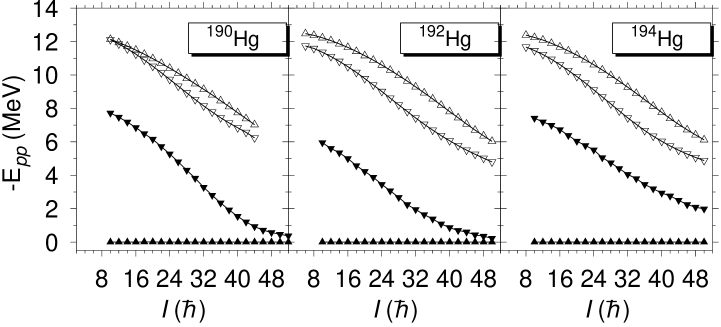
Figure 1: Particle-particle correlation energies for ^190-192-194Hg. Full triangles : CHFB pairing energy for protons (upwards) and neutrons (downwards). Empty triangles : CHFBLN pairing energy for protons (upwards) and neutrons (downwards).

In the CHFB approach we do not find pairing correlations for the proton system for the nuclei considered. For the neutron system we find sizable pairing correlations at low and medium spins which diminish at large angular momentum due to a strong Coriolis antipairing effect, at very high spins they get very small. In the CHFBLN approach, we find larger correlation energy for both, the proton and neutron systems, we also observe the Coriolis antipairing effect as the angular momentum increases but the systems remain correlated even at the largest spins. We also realize that the LN term has a larger effect on the proton system than on the neutron one.

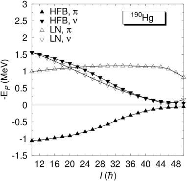
Figure 2: Pairing energies, eq. (58), for ¹⁹⁰Hg. Full triangles : CHFB pairing energy for protons (upwards) and neutrons (downwards). Empty triangles : CHFBLN pairing energy for protons (upwards) and neutrons (downwards).

The energy $E_{pp}$ is a measure of the pairing correlations, but there are other ways to look for pair correlations. In the scientific literature, and in the scope of HFB theories, the pairing energy $E_{P}$ is defined as

$$E_{P}=E-E_{HF}$$ (58)

with $E$ the energy calculated in the HFB (or LN) approximation and $E_{HF}$ the energy calculated in the Hartree-Fock approach. This quantity is different from what we have called particle-particle correlation energy $E_{pp}$. The quantities $E_{P}$ and $E_{pp}$ coincide only in the case of a BCS calculation performed on top of a HF solution, i.e. without selfconsistency in the Hartree-Fock and the pairing fields.

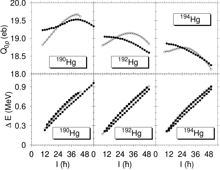
Figure 3: Results for ^190-192-194Hg. Upper panel : The charge quadrupole moment versus the angular moment. Full (empty) circles represent the CHFB (CHFBLN) approach. Lower panel : Gamma-ray energy $\Delta E_{I}=E(I)-E(I-2)$ as a function of the angular momentum. Full (open) circles stand for the CHFB (CHFBLN) results and full squares for the experimental data, for ¹⁹⁰Hg [31], for ¹⁹⁰Hg [33] and for ¹⁹⁴Hg [34] .

In fig. 2, as an example, we display the quantity $E_{P}$ for ¹⁹⁰Hg, in the HFB and the LN approach for protons and neutrons. In the HFB solution we have found a superfluid solution in the neutron channel but not in the proton channel. The HF solution provides the proton and neutron densities, $\rho_{Z}$ and $\rho_{N}$, that minimize the energy in the absence of pairing correlations. We expect, therefore, the proton contribution to the total energy to be deeper in the HF than in the HFB approach, the neutron contribution, on the contrary, must be deeper in the HFB than on the HF approach. The total energy must be, obviously, deeper in the HFB than in the HF approach. We observe in fig. 2 that these expectations are fulfilled. We also find a slow convergence to zero in the energy $E_{P}$, as a function of the angular momentum, indicating the quenching of the pairing correlations. In the LN approach we find the neutron system to behave very similarly to the HFB one, the proton one behaves differently as expected from the behavior of $E_{pp}$. It is interesting to point out that $E_{P}$, a quantity with more physical content than $E_{pp}$, is much smaller than $E_{pp}$ as one would expect from the experimental data. It is important to notice that whereas the correlation energy gained by the HFB procedure with respect to HF is only of 0.5 MeV at $I=12\hbar$, the correlation energy gained by the LN procedure with respect to HFB at the same spin is of 2.0 MeV. This result indicates the relevance of the restoration of the particle number symmetry in this case.

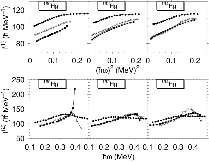
Figure 4: Upper panel : the static moment of inertia, ${\cal I}^{(1)}(I)=(2I-1)/\Delta E_{I}$ versus the square of the angular frequency, $\hbar\omega(I)=\Delta E_{I}/2$. Lower panel : Second moments of inertia, ${\cal I}^{(2)}(I)=4/(\Delta E_{I}-\Delta E_{I-2})$, for ^190-192-194Hg. The meaning of the symbols is the following : Squares for the experimental data [31], [33], [34], full (empty) circles for the CHFB (CHFBLN) approach.

In the upper part of fig. 3 we show the angular momentum dependence of the quadrupole moment, $Q_{0p}$, for the nuclei ^190-192-194Hg. With increasing neutron number we observe a global decrease in deformation and a reduction in the $I$-values in which the quadrupole moment starts to decrease. The CHFBLN and the CHFB results differ mostly at low spins where the pairing correlations are larger. This causes the crossing of the results of both calculations for each nucleus. As a function of the angular momentum we observe first an increase of the quadrupole moment due to a reduction of the pairing correlations and then a decrease of $Q_{0p}$. This anti-stretching effect is caused by the Coriolis force. The CHFB and the CHFBLN predictions are slightly higher than the experimental values $17.7^{+1}_{-1.2}$ eb for¹⁹⁰Hg [30], $17.7\pm 0.8$ eb for¹⁹²Hg [32] and $17.7\pm 0.4$ eb for¹⁹⁴Hg [32]. These quadrupole moments correspond to $\beta$ deformations along the yrast band of $0.560-0.580$, $0.555-0.565$, $0.540-0.552$ for ^190-192-194Hg respectively, the gamma deformation remains zero for the three nuclei at all spin values.

In the lower part of fig. 3 we display the transition energies versus the angular momentum. The agreement with the experimental data is good in the CHFBLN approach, in the CHFB one obtains too low values. The reason for this behavior is again the smallness of the pairing correlation in the CHFB approach as it can be seen in the upper part of fig. 4 where we display the static moments of inertia versus the square of the angular frequency $\hbar\omega$. Here we observe that the CHFB moments of inertia are too large as compared with the experiment. The CHFBLN moments of inertia are in much better agreement with the experiment, specially for ^192-194Hg.

Figure 5: Quasiparticles energies for the nuclei ¹⁹⁰Hg (upper panel) ¹⁹²Hg (middle panel) and ¹⁹⁴Hg (lower panel), in the left hand side for positive parity protons and in the right hand side for negative parity neutrons. The continuous (dashed) lines correspond to positive (negative) signature.

In the lower part of fig. 4, the second moment of inertia ${\cal I}^{(2)}$ as a function of the angular frequency is represented. Here, as in the previous picture, the CHFB results are in poor agreement with the experiment. At small spin values the moment of inertia is too large and the neutron alignment sets in too early. The CHFBLN results, however, are in very good agreement with the experimental results, the correlations induced by the Lipkin-Nogami prescription produce the desired effect, namely, to diminish the moment of inertia at small spin values and to delay the alignment to higher spin values. For ¹⁹⁰Hg the experimental results show a sharp upbending at $I=42\hbar$ ( $\hbar\omega\approx 0.4$ MeV ), in our calculations we do not get a sharp upbending but a modest one, we see however a clear discontinuity in the ${\cal I}^{(2)}$ at $I=44\hbar$. For the last points of our calculations there are not experimental results. One expects, however, that after the sharp backbending the experimental results will bend down. The CHFBLN for ¹⁹²Hg are in very good agreement with the experimental ones and for ¹⁹⁴Hg we get slightly more alignment at high spins than in the experiment.

To investigate the orbitals responsible for the alignments we display in fig. 5 the quasiparticle energies for the three nuclei. We find that the orbitals responsible for the alignment at $\hbar\omega\approx 0.4$ MeV are the $N=7$ ones, mainly the $\nu[761]\frac{3}{2}$ for ¹⁹⁰Hg and ¹⁹²Hg and the $\nu[752]\frac{5}{2}$ for ¹⁹⁴Hg, though it is hard to distinguish both orbitals because they are strongly mixed. These results are in good agreement with the ones obtained in [3]. The proton alignment takes place at higher frequencies ($\hbar\omega\approx 0.45$).

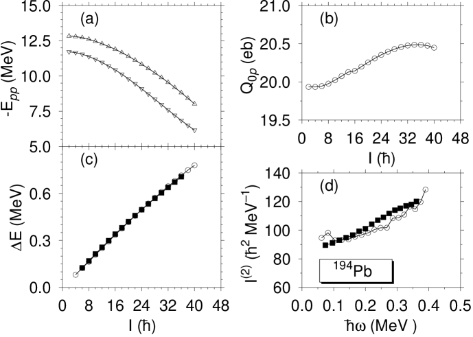
Figure 6: The nucleus ¹⁹⁴Pb in the CHFBLN approximation. (a) The particle-particle correlation energy for protons (triangles) and neutrons (inverted triangles) (b) The charge quadrupole moment, (c) the transition energy, the experimental data are from [36] and (d) the dynamical moment of inertia

As a further example of this region we display in fig. 6 the results for the nucleus ¹⁹⁴Pb in the CHFBLN approximation. The particle-particle correlation energy $E_{pp}$, fig. 6a, shows a similar behavior to the Hg isotopes, i.e., a modest Coriolis antipairing effect at small spins which becomes larger at high angular momentum. The quadrupole moment behaves similarly to the previous studied nuclei : first, it increases as a consequence of the weakening of the pairing correlations and at high angular momentum starts to decrease due to the anti-stretching effect. The numerical value of $Q_{0p}$ is also a little larger than the experimental value of $18.8\pm 1.1$ eb, [35]. The transition energies are depicted in fig. (6c), here the agreement with the experimental data is excellent. Finally, in fig. (6d) the dynamical moment of inertia is shown, we find a very good agreement with the experimental data at low and high angular momentum. The analysis of the quasiparticles energies as a function of the angular momentum, indicates that in this case the orbital responsible for the alignment at high spin is the $\nu[752]\frac{5}{2}$.

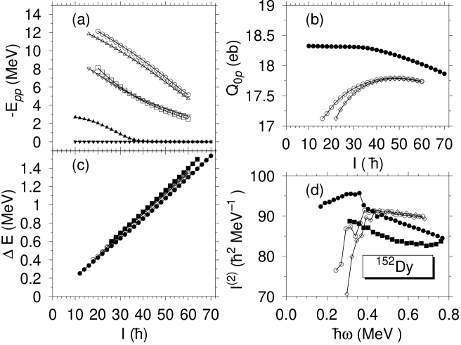
Figure 7: The nucleus ¹⁵²Dy in the LN and the HFB approximations. (a) The particle-particle correlation energy in CHFBLN (CHFBLNFD) for protons, open triangles (circles) and neutrons, empty inverted triangles (squares). Same quantity in CHFB : protons, triangles; neutrons, inverted triangles. (b) The charge quadrupole moment, CHFBLN (empty circles), CHFBLNFD (squares) and CHFB (full circles). (c) the transition energy. Experiment (full squares) [41], CHFBLN (empty circles), CHFBLNFD (empty squares), CHFB (full circles) and (d) the dynamical moment of inertia. Same symbols as in (c).

3.2 The $A=150$ region.

We shall now turn to the $A=150$ region. This region is characterized by smaller pairing correlations, the restoration of particle number symmetry should not be, therefore, as relevant as in the $A=190$ region. As examples of this region we discuss the nuclei ¹⁵²Dy and ¹⁵⁰Gd.

As mentioned at the beginning of this section, we would like to compare, in the $A=150$ region, the results obtained with the two approaches to the problem of the density dependence of the Hamiltonian discussed in the theory section.

In fig. 7 we represent the main results for the nucleus ¹⁵²Dy in the HFB and in the LN approach. The LN results with the prescription of the many-body density dependence we shall call CHFBLN, as before, and those based in the functional of the density prescription, CHFBLNFD.

The particle-particle correlation energy, $E_{pp}$, is represented in fig. 7a as a function of the angular momentum. In the CHFB approximation, the neutron system is not correlated while the proton one is slightly correlated for spin values smaller than $36\hbar$. In the LN approximation, however both systems are correlated. The results in the CHFBLNFD and CHFBLN are very similar for protons and neutrons. As expected we obtain smaller correlation energies in this region than in the $A=190$ one. In fig. 8 we plot the energy $E_{P}$ of eq. (58) in the CHFBLN approach. For neutrons is very small for all spin values and for protons around 1.8 MeV at spin $40\hbar$ and it decreases to 1.5 MeV for spin $60\hbar$, i.e. the energy gain allowing superfluid wave functions is about 2 MeV.

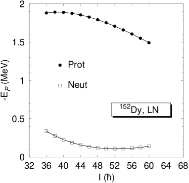
Figure 8: Pairing energies, Eq. (58), for ¹⁵²Dy in the CHFBLN approximation for protons (dots) and neutrons (squares).

In fig. 7b we display the charge quadrupole moment, $Q_{0p}$, versus the angular momentum. In the CHFB approximation and at small angular momentum it is almost constant, only around spins values of $30\hbar$, $Q_{0p}$ starts to decrease by the Coriolis anti-stretching effect. In the CHFBLN approaches the behavior at low spins is quite different (it increases due to the Coriolis antipairing effect) and only around spin values of $50\hbar$ starts to decrease. The experimental value is $17.5\pm 0.2$ eb, [39, 40], in good agreement with the CHFBLN results, the HFB values being somewhat larger. The nuclei are axially symmetric, i.e. the gamma deformation is zero. In fig. 7c the gamma ray energies are plotted versus the angular momentum. The HFB predictions are the lowest ones due to the large moment of inertia. The CHFBLN results are slightly below the experimental data and almost parallel to them. Both CHFBLN approaches to the gamma ray energies practically coincide. Finally in fig. 7d the second moments of inertia are displayed versus the angular frequency. The CHFB results are larger than the experimental ones but they behave in a similar way. The inclusion of additional pairing correlations through the LN approach produces an enhancement of the second moment of inertia as compared with the CHFB results. This anomalous behavior has been also found in [7]. The two LN approaches are very similar at high spin values, only at small spins one finds differences. The low values of ${\cal I}^{(2)}$ at small angular frequencies are probably due to an excess of pair correlations at low $I$, as one can also see in the behavior of the quadrupole moment, fig. 7b, ${\cal I}^{(2)}$ being a second derivative magnifies small effects. The first moment of inertia, fig. 7c, however, has very reasonable values. Concerning the quality of the LN approaches, we may conclude, as in the $A=190$ region that both approaches practically coincide.

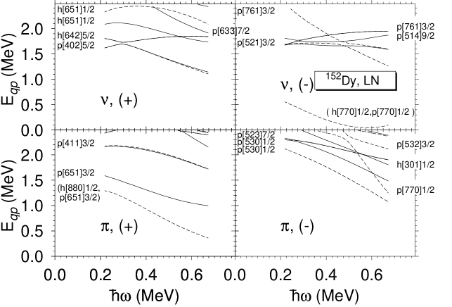
Figure 9: Quasiparticles energies for the nucleus ¹⁵²Dy, in the upper part for protons and in the lower part for neutrons. The continuous (dashed) lines correspond to positive (negative) signature.

In fig. (9) the quasiparticle energies for the nucleus ¹⁵²Dy are represented versus de angular frequency. From these levels one can predict the blocking structure of the excited bands in this nucleus or in the nearby odd-even nuclei. One should be aware, however, that there is strong mixing within the Nilsson levels and that the character of particle or hole near the Fermi surface, in the presence of pairing correlations, is not a precise statement. Most of the levels shown in the figure coincide with the assignment proposed [41, 42].

The next example in the $A=150$ region is the ¹⁵⁰Gd, the results are shown in fig. 10. Since we have seen in the previous example that both density prescriptions provide similar results, for this nucleus we only show the results with the many body density prescription. In fig. 10a, the CHFBLN pairing energies versus the angular momentum are represented, they show an smooth decrease with growing angular momentum. In fig. 10b, the charge quadrupole moments as a function of $I$ are presented. They display the typical Coriolis effects: first an increase caused by the Coriolis antipairing effect and later one the Coriolis antistretching effect. It is in good agreement with the experimental value, $17^{+0.5}_{-0.4}$ eb, [37]. This nucleus is also axially symmetric. The transition energies represented in fig. 10c are well reproduced by the theoretical predictions, indicating, nevertheless, a slightly larger moment of inertia than the experiment. The second moment of inertia is shown in fig. 10d, the agreement is good except at the lowest values of the angular momentum, where the experimental points present a sharper level crossing than in the theory.

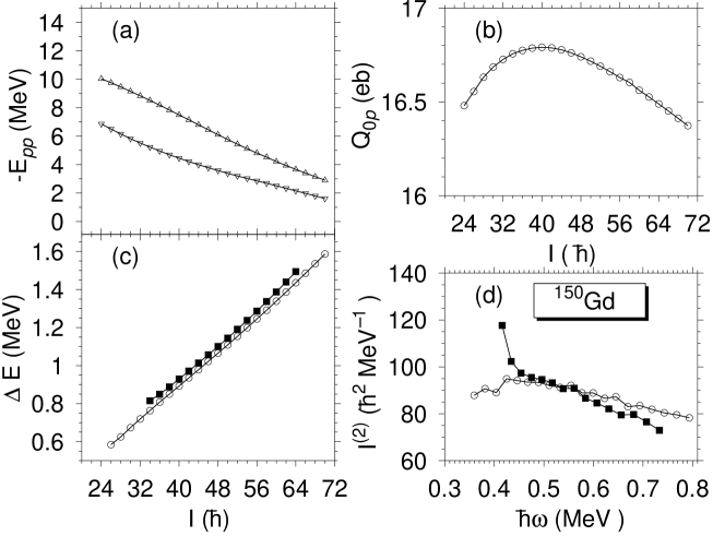
Figure 10: The nucleus ¹⁵⁰Gd in the CHFBLN approximation. (a) The particle-particle correlation energy for protons (triangles) and neutrons (inverted triangles) (b) The charge quadrupole moment, (c) the transition energy, the experimental data [38] are represented by squares and (d) the dynamical moment of inertia

4 Conclusions

In conclusion, we have discussed the Lipkin-Nogami equations for density dependent forces and two different prescriptions for the density dependence of the Hamiltonian to be used in the evaluation of non-diagonal matrix elements.

As an application we have analyzed the high spin properties of the nuclei ^190-192-194Hg and ¹⁹⁴Pb of the $A=190$ region and the nuclei ¹⁵²Dy and ¹⁵⁰Gd of the $A=150$ region in the Cranked Hartree-Fock-Bogoliubov and the Cranked Lipkin-Nogami approaches.

Global properties as well as sensitive properties as the second moment of inertia are well reproduced, specially within the CHFBLN approximation. In general we obtain excellent qualitative agreement with the experiment and in some cases a quantitative one. The approximate restoration of the particle number symmetry is the essential ingredient for the quantitative agreement. We believe that the Gogny force with the approximate particle number projected mean field theory provides a good description of nuclear properties under a large variety of situations.

This work was supported in part by DGICyT, Spain under Project PB97–0023. One of us (A.V.) would like to thank the Spanish Ministerio de Asuntos Exteriores for financial support through an ICI grant.

5 Appendix A :Lagrange multiplier with density dependent forces

In the HFB theory the wave function $|\Phi\rangle$ that minimizes the energy with the constraint of providing the right particle number on the average is given by

$$\delta\langle\Phi|\hat{H}-\lambda\hat{N}|\Phi\rangle=0$$ (59)

for density dependent forces one obtains

$$\langle\delta\Phi|\hat{H}|\Phi\rangle+\left\langle\Phi\left|\frac{\partial H(\rho)}{\partial\rho(r)}\langle\delta\Phi|\hat{\rho}|\Phi\rangle\right|\Phi\right\rangle-\lambda\langle\delta\Phi|\hat{N}|\Phi\rangle=0$$ (60)

this equation must hold for any arbitrary variation $|\delta\Phi\rangle$, in particular for $|\delta\Phi\rangle=\Delta\hat{N}|\Phi\rangle$, substitution in eq. (60) provides

$$\lambda=\frac{\langle\Phi|\hat{H}\Delta\hat{N}|\Phi\rangle}{\langle\Phi|(\Delta\hat{N})^{2}|\Phi\rangle}+\left\langle\Phi\left|\frac{\partial H(\rho)}{\partial\rho(r)}\frac{\langle\Phi|\hat{\rho}\Delta\hat{N}|\Phi\rangle}{\langle\Phi|(\Delta\hat{N})^{2}|\Phi\rangle}\right|\Phi\right\rangle.$$ (61)

6 Appendix B : Functionals of the density

We want to define a prescription to evaluate overlaps of the hamiltonian

$$\frac{\left\langle\Phi|\hat{H}|\Phi^{\prime}\right\rangle}{\left\langle\Phi|\Phi^{\prime}\right\rangle},$$

for density dependent forces where both $\left|\Phi\right\rangle$ and $\left|\Phi^{\prime}\right\rangle$ are product wave functions of the HFB type. The philosophy behind the prescription is that a density dependent force does not define a hamiltonian but rather the energy, which is a functional of the density and the pairing tensor

$$E[\rho,\kappa]=\sum_{k_{1}k_{2}}T_{k_{1}k_{2}}\rho_{k_{2}k_{1}}+\frac{1}{4}\sum_{k_{1}k_{2}k_{3}k_{4}}\overline{\nu}_{k_{1}k_{2}k_{3}k_{4}}\left(2\rho_{k_{4}k_{2}}\rho_{k_{3}k_{1}}+\kappa_{k_{3}k_{4}}\kappa^{*}_{k_{1}k_{2}}\right)$$ (62)

where the two-body interaction could depend upon the spatial density $\rho(\vec{r})$ to some power $\alpha$, $v[\rho^{\alpha}(\vec{r})]$, as is the case for the Gogny force. In the above expression the spatial density is defined in the usual way

$$\rho(\vec{r})=\frac{\left\langle\Phi|\hat{\rho}|\Phi\right\rangle}{\left\langle\Phi|\Phi\right\rangle}=\sum_{k_{1}k_{2}}f_{k_{1}k_{2}}(\vec{r})\rho_{k_{2}k_{1}},$$

where the density operator is given by

$$\hat{\rho}(\vec{r})=\sum^{A}_{i=1}\delta(\vec{r}-\vec{r}_{i})=\sum_{k_{1}k_{2}}f_{k_{1}k_{2}}(\vec{r})c^{+}_{k_{1}}c_{k_{2}}.$$

The formal evaluation of the hamiltonian overlap for non-density dependent forces is straightforward. Using the extended Wick theorem, one gets

$$\frac{\left\langle\Phi|\hat{H}|\Phi^{\prime}\right\rangle}{\left\langle\Phi|\Phi^{\prime}\right\rangle}=\sum_{k_{1}k_{2}}T_{k_{1}k_{2}}\widetilde{\rho}_{k_{2}k_{1}}+\frac{1}{4}\sum_{k_{1}k_{2}k_{3}k_{4}}\overline{\nu}_{k_{1}k_{2}k_{3}k_{4}}\left(2\widetilde{\rho}_{k_{4}k_{2}}\widetilde{\rho}_{k_{3}k_{1}}+\widetilde{\kappa}_{k_{3}k_{4}}\widetilde{\overline{\kappa}}_{k_{1}k_{2}}\right),$$ (63)

where

$$\widetilde{\rho}_{k_{3}k_{1}}=\frac{\left\langle\Phi|c^{+}_{k_{1}}c_{k_{3}}|\Phi^{\prime}\right\rangle}{\left\langle\Phi|\Phi^{\prime}\right\rangle},\;\;\;\widetilde{\kappa}_{k_{3}k_{4}}=\frac{\left\langle\Phi|c_{k_{4}}c_{k_{3}}|\Phi^{\prime}\right\rangle}{\left\langle\Phi|\Phi^{\prime}\right\rangle},\;\;\;\widetilde{\overline{\kappa}}_{k_{1}k_{2}}=\frac{\left\langle\Phi|c^{+}_{k_{1}}c^{+}_{k_{2}}|\Phi^{\prime}\right\rangle}{\left\langle\Phi|\Phi^{\prime}\right\rangle}.$$ (64)

Therefore, for non-density dependent forces both, the energy, eq. (62) and the hamiltonian overlap, eq. (63), are given by the same functional of the density matrix and the pairing tensor but evaluated with the corresponding densities and pairing tensors. Inspired by these results we use the following prescription for density dependent forces : in the evaluation of the hamiltonian overlap a density dependent interaction depending upon $\widetilde{\rho}$, eq. (64), must be used. From the point of view of defining a hamiltonian the previous prescription amounts to use the density

$$\widetilde{\rho}(\vec{r})=\frac{\left\langle\Phi|\hat{\rho}(\vec{r})|\Phi^{\prime}\right\rangle}{\left\langle\Phi|\Phi^{\prime}\right\rangle}$$

for the density dependent part of the hamiltonian. This prescription coincides with the one obtained for a Skyrme force with a linear dependence in $\rho$. The above density is, in general, not a real quantity rendering the density dependent “hamiltonian” a non hermitian operator. This is not a real problem as the hamiltonian overlap can be a complex quantity, we only have to be sure that the projected energy is a real quantity as it will be shown below.

Another important check concerning the consistency of the prescription is the following : since $\hat{P}^{N}$ and the density dependent hamiltonian do commute and $\hat{P}^{N^{2}}=\hat{P}^{N}$, we may write

$$E_{N}=\frac{\left\langle\psi_{N}\right|\hat{H}\left|\psi_{N}\right\rangle}{\left\langle\psi_{N}|\psi_{N}\right\rangle}=\frac{\left\langle\Phi\right|\hat{H}\left|\psi_{N}\right\rangle}{\left\langle\Phi\right.\left|\psi_{N}\right\rangle}.$$ (65)

According to our prescription, to evaluate non-diagonal matrix elements of the first expression of $E_{N}$ in eq. (65), in the hamiltonian we have to consider the density

$$\widetilde{\rho}_{\phi,\phi^{\prime}}(\vec{r})=\frac{\left\langle\Phi\right|e^{-i\phi\hat{N}}\hat{\rho}(\vec{r})e^{i\phi^{\prime}\hat{N}}\left|\Phi\right\rangle}{\left\langle\Phi\right|e^{i(\phi^{\prime}-\phi)\hat{N}}\left|\Phi\right\rangle},$$ (66)

whereas for the non-diagonal matrix elements of the second expression of $E_{N}$ in eq. (65) one should use

$$\widetilde{\rho}_{\phi}(\vec{r})=\frac{\left\langle\Phi\right|\hat{\rho}(\vec{r})e^{i\phi\hat{N}}\left|\Phi\right\rangle}{\left\langle\Phi\right|e^{i\phi\hat{N}}\left|\Phi\right\rangle}.$$ (67)

The final result, should be independent of whether we use the first or the second expression. This is clearly true, since eq. (66) can be written as

$$\widetilde{\rho}_{0,\phi^{\prime}-\phi}(\vec{r})=\frac{\left\langle\Phi\right|\hat{\rho}(\vec{r})e^{i(\phi^{\prime}-\phi)\hat{N}}\left|\Phi\right\rangle}{\left\langle\Phi\right|e^{i(\phi^{\prime}-\phi)\hat{N}}\left|\Phi\right\rangle},$$

due to the commutativity of $e^{i\phi\hat{N}}$ with $\hat{\rho}(\vec{r})$. The operator $e^{i\phi\hat{N}}$ also commutes with $\widetilde{\rho}_{0,\phi^{\prime}-\phi}(\vec{r})$ showing that

$$h(\phi,\phi^{\prime}) = \left\langle\Phi\right|e^{-i\phi\hat{N}}\hat{H}[\widetilde{\rho}_{\phi,\phi^{\prime}}(\vec{r})]e^{i\phi^{\prime}\hat{N}}\left|\Phi\right\rangle=\left\langle\Phi\right|\hat{H}[\widetilde{\rho}_{0,\phi^{\prime}-\phi}(\vec{r})]e^{i(\phi^{\prime}-\phi)\hat{N}}\left|\Phi\right\rangle$$

$$= h(0,\phi^{\prime}-\phi)$$

which is the property needed to obtain the second expression of Eq (65). Obviously, we shall use the second expression for the projected energy and eq. (67), for the density entering in the density dependent part of the interaction, in the evaluation of $h(\phi)$.

Next, in order to ensure the reality of the projected energy, we have to show that the following property holds

$$h^{*}(\phi)=h(-\phi).$$ (68)

The complex conjugate of $\widetilde{\rho}_{\phi}(\vec{r})$ is given by

$$\widetilde{\rho}^{*}_{\phi}(\vec{r})=\frac{\left\langle\Phi\right|e^{-i\phi\hat{N}}\hat{\rho}(\vec{r})\left|\Phi\right\rangle}{\left\langle\Phi\right|e^{-i\phi\hat{N}}\left|\Phi\right\rangle}=\frac{\left\langle\Phi\right|\hat{\rho}(\vec{r})e^{-i\phi\hat{N}}\left|\Phi\right\rangle}{\left\langle\Phi\right|e^{-i\phi\hat{N}}\left|\Phi\right\rangle}=\widetilde{\rho}_{-\phi}(\vec{r}),$$

using this property in the definition of $h^{*}(\phi)$, Eq (68) is demonstrated,

$$h^{*}(\phi)=\left\langle\Phi\right|e^{-i\phi\hat{N}}\hat{H}(\widetilde{\rho}^{*}_{\phi}(\vec{r}))\left|\Phi\right\rangle=\left\langle\Phi\right|\hat{H}(\widetilde{\rho}_{-\phi}(\vec{r}))e^{-i\phi\hat{N}}\left|\Phi\right\rangle=h(-\phi).$$

7 Appendix C: Evaluation of $\left\langle\Delta\hat{H}(\Delta\hat{N})^{2}\right\rangle$

In order to evaluate $\left\langle\Delta\hat{H}(\Delta\hat{N})^{2}\right\rangle$ we will use the following relation

$$\left\langle\Delta\hat{H}(\Delta\hat{N})^{2}\right\rangle=-\frac{\partial^{2}}{\partial\phi^{2}}\left.\frac{\left\langle\Phi\right|\hat{H}e^{i\phi\hat{N}}\left|\Phi\right\rangle}{\left\langle\Phi\right|e^{i\phi\hat{N}}\left|\Phi\right\rangle}\right|_{\phi=0}.$$ (69)

In this expression the density appearing in the density dependent part of the hamiltonian is, obviously $\langle\Phi|c^{+}(\vec{r})c(\vec{r})|\Phi\rangle$. The matrix element of the right hand side is given by eq. (63) with $|\Phi^{\prime}\rangle=e^{i\phi\hat{N}}|\Phi\rangle$. We may further write

$$\frac{\left\langle\Phi\right|\hat{H}e^{i\phi\hat{N}}\left|\Phi\right\rangle}{\left\langle\Phi\right|e^{i\phi\hat{N}}\left|\Phi\right\rangle}=Tr\left[(T+\frac{1}{2}\Gamma(\phi))\widetilde{\rho}(\phi)\right]-\frac{1}{2}Tr\left[\Delta(\phi)\widetilde{\overline{\kappa}}(\phi)\right],$$

where we have introduced the notation

$$\Delta_{k_{1}k_{2}}(\phi)=\frac{1}{2}\sum_{k_{3}k_{4}}\overline{\nu}_{k_{1}k_{2}k_{3}k_{4}}\widetilde{\kappa}_{k_{3}k_{4}}(\phi),\;\;\;\;\;\Gamma_{k_{1}k_{2}}(\phi)=\sum_{k_{3}k_{4}}\overline{\nu}_{k_{1}k_{3}k_{2}k_{4}}\widetilde{\rho}_{k_{4}k_{3}}(\phi).$$

Performing the second derivative with respect to $\phi$ and taking the limit $\phi=0$ we obtain

$$\frac{\partial^{2}}{\partial\phi^{2}}\left.\frac{\left\langle\Phi\right|\hat{H}e^{i\phi\hat{N}}\left|\Phi\right\rangle}{\left\langle\Phi\right|e^{i\phi\hat{N}}\left|\Phi\right\rangle}\right|_{\phi=0}= - Tr\left[T\rho_{2N}+\frac{1}{2}(\Gamma_{2N}\rho+\Gamma\rho_{2N}+2\Gamma_{N}\rho_{N})\right]$$ (70)

$$+ \frac{1}{2}Tr[\Delta_{2N}\kappa^{*}+\Delta\overline{\kappa}_{2N}+2\Delta_{N}\overline{\kappa}_{N}],$$

where we have introduced the matrices

$$\left(\rho_{N}\right)_{k_{1}k_{2}} = \frac{1}{i}\left.\frac{\partial}{\partial\phi}\widetilde{\rho}_{k_{1}k_{2}}(\phi)\right|_{\phi=0}=\left\langle\Phi\right|c^{+}_{k_{2}}c_{k_{1}}\Delta\hat{N}\left|\Phi\right\rangle,$$

$$\left(\kappa_{N}\right)_{k_{1}k_{2}} = \frac{1}{i}\left.\frac{\partial}{\partial\phi}\widetilde{\kappa}_{k_{1}k_{2}}(\phi)\right|_{\phi=0}=\left\langle\Phi\right|c_{k_{2}}c_{k_{1}}\Delta\hat{N}\left|\Phi\right\rangle,$$

$$\left(\overline{\kappa}_{N}\right)_{k_{1}k_{2}} = \frac{1}{i}\left.\frac{\partial}{\partial\phi}\widetilde{\overline{\kappa}}_{k_{1}k_{2}}(\phi)\right|_{\phi=0}=\left\langle\Phi\right|c^{+}_{k_{1}}c^{+}_{k_{2}}\Delta\hat{N}\left|\Phi\right\rangle,$$

and

$$\left(\rho_{2N}\right)_{k_{1}k_{2}} = -\left.\frac{\partial^{2}}{\partial\phi^{2}}\widetilde{\rho}_{k_{1}k_{2}}(\phi)\right|_{\phi=0}=\left\langle\Phi\right|\Delta\left(c^{+}_{k_{2}}c_{k_{1}}\right)\left(\Delta\hat{N}\right)^{2}\left|\Phi\right\rangle,$$

$$\left(\kappa_{2N}\right)_{k_{1}k_{2}} = -\left.\frac{\partial^{2}}{\partial\phi^{2}}\widetilde{\kappa}_{k_{1}k_{2}}(\phi)\right|_{\phi=0}=\left\langle\Phi\right|\Delta\left(c_{k_{2}}c_{k_{1}}\right)\left(\Delta\hat{N}\right)^{2}\left|\Phi\right\rangle,$$

$$\left(\overline{\kappa}_{2N}\right)_{k_{1}k_{2}} = -\left.\frac{\partial^{2}}{\partial\phi^{2}}\widetilde{\overline{\kappa}}_{k_{1}k_{2}}(\phi)\right|_{\phi=0}=\left\langle\Phi\right|\Delta\left(c^{+}_{k_{1}}c^{+}_{k_{2}}\right)\left(\Delta\hat{N}\right)^{2}\left|\Phi\right\rangle,$$

$\Gamma_{N},\Gamma_{2N},\Delta_{N}$ and $\Delta_{2N}$ are given by the usual expressions but the traces have to be taken with $\rho_{N},\rho_{2N},\kappa_{N}$ and $\kappa_{2N}$ respectively.

References

- [1] P. Bonche, P.-H. Heenen and H.C. Flocard. Nucl. Phys. A467, 115 (1987).
- [2] H.C. Flocard. Nuclear Structure of the Zirconium Region, J. Eberth, R.A. Meyer and K. Sistemich (Eds.). Research Reports in Physics. Springer-Verlag, p 143 (1988).
- [3] J. Terasaki, P.-H. Heenen, P. Bonche, J. Dobaczewski and H. Flocard, Nucl. Phys. A593 (1995) 1-20
- [4] P.-H.Heenen, J.Dobaczewski, W.Nazarewicz, P.Bonche, T.L.Khoo, Phys.Rev. C57 (1998)1719
- [5] C. Rigollet, P.Bonche, H.Flocard, P.-H.Heenen, Phys.Rev. C59 (1999) 3120
- [6] R. R. Chasman, Phys. Lett. B319 (1993)134.
- [7] P. Bonche, H. Flocard and P.-H. Heenen, Nucl. Phys. A598 (1996) 169
- [8] B.R. Mottelson and J.G. Valatin. Phys. Rev. Lett. 5, 511 (1960).
- [9] D. Gogny. Nuclear Selfconsistent Fields. Eds. G. Ripka and M. Porneuf (North Holland 1975).
- [10] J. Dechargé and D. Gogny. Phys. Rev. C21, 1568 (1980).
- [11] J.F. Berger, M. Girod and D. Gogny. Nucl. Phys. A428, 23c (1984).
- [12] J. L. Egido and L. M. Robledo, Phys. Rev. Lett. 70, 2876 (1993).
- [13] J. L. Egido, L. M. Robledo and R.R. Chasman, Phys. Lett. B322 (1994) 22-26
- [14] M. Girod, J.P. Delaroche, J. F. Berger and J. Libert, Phys. Lett. B325 (1994) 1-6
- [15] A. Valor, J.L. Egido and L.M. Robledo, Phys. Rev. C53, 172 (1996).
- [16] A. Valor, J.L. Egido and L.M. Robledo, Phys. Lett. B392, 249-254 (1997).
- [17] P. Ring and P. Schuck, The Nuclear Many Body Problem (1980), Springer–Verlag Edt. Berlin.
- [18] J.L. Egido and P. Ring, Nucl. Phys. A388, 19 (1982).
- [19] A. Kamlah, Z. Phys. 216, 52 (1968).
- [20] D. C. Zheng, D.W.L. Sprung and H. Flocard, Phys. Rev. C46, 1335 (1992).
- [21] H. J. Lipkin, Ann. Phys. (N.Y.) 12, 425 (1960).
- [22] Y. Nogami, Phys. Rev. B134, 313 (1964); Y. Nogami and I.J. Zucker, Nucl. Phys. 60, 203 (1964).
- [23] J. F. Goodfellow and Y. Nogami, Can. J. Phys. 44, 1321 (1966).
- [24] P. Magierski, S. Cwiok, J. Dobaczewski and W. Nazarewicz, Phys. Rev. C48, 1681 (1993).
- [25] G. Gall, P. Bonche, J. Dobaczewski, H. Flocard and P.-H. Heenen, Z. Phys. A348, 183 (1994).
- [26] P. Bonche, J. Dobaczewski, H. Flocard, P.-H. Heenen and J. Meyer, Nucl. Phys. A510, 466 (1990).
- [27] A. Valor, Ph. D. Thesis, Universidad Autónoma de Madrid, 1996, unpublished.
- [28] J.L. Egido, J. Lessing, V. Martin and L.M. Robledo, Nucl. Phys. A594 (1995)70-86
- [29] J.F. Berger, M. Girod and D. Gogny, Comp. Phys. Comm. 63(1991) 365-374
- [30] H. Amro et al. Phys. Lett B413 (1997) 15
- [31] B. Crowell et al., Phys. Rev C51(1995) R1599
- [32] E. F. Moore et al. Phys. Rev. C55 (1997) R2150
- [33] P. Fallon et al., Phys. Rev. C51, R1609 (1995)
- [34] B. Cederwall et al., Phys. Rev. Lett. 72 (1994) 3150
- [35] R. Krucken et al., Phys. Rev. C55 (1997) R1625
- [36] R. Krucken et al., Phys. Lett. B345 (1995) 124
- [37] C.W. Beausang et al., Phys.Lett. 417B (1998) 13
- [38] P. Fallon et al., Phys. Lett. B218 (1989) 137
- [39] H. Savajols et al., Phys. Rev. Lett. 76 (1996) 4480
- [40] D. Nisius at al., Phys. Lett. 392B (1997) 18
- [41] P.J. Dagnall et al., Phys. Lett. B335 (1994) 313
- [42] A.V. Afanasjev, J. König and P. Ring, Nucl. Phys. A608 (1996)107