Parameter Counting in Relativistic
Mean-Field Models

Abstract

Power counting is applied to relativistic mean-field energy functionals to estimate contributions to the energy from individual terms. New estimates for isovector, tensor, and gradient terms in finite nuclei are shown to be consistent with direct, high-quality fits. The estimates establish a hierarchy of model parameters and identify how many parameters are well constrained by bulk nuclear observables. We conclude that four (possibly five) isoscalar, non-gradient parameters, one gradient parameter, and one isovector parameter are well determined by the usual bulk nuclear observables.

I Introduction and Motivation

Relativistic mean-field (RMF) descriptions of the nuclear many-body problem have existed for nearly fifty years [1]. An extensive body of work [2, 3, 4] has shown that RMF theories can realistically reproduce the bulk and single-particle properties of medium to heavy nuclei. Successful RMF theories are characterized by large, neutral, Lorentz scalar and vector potentials (roughly several hundred MeV at nuclear equilibrium density), a new saturation mechanism for nuclear matter that arises from relativistic (i.e., velocity-dependent) interaction effects from the scalar potential, and a nuclear spin-orbit force that is determined by this velocity dependence. The vector potential provides an efficient representation of the short-range nucleon–nucleon (NN) repulsion, while the scalar potential provides the mid-range NN attraction by simulating correlated, scalar-isoscalar two-pion exchange, which is the most important pionic contribution for describing the bulk properties of nuclear matter.

For many years, RMF model parameters were determined by fitting them to the properties of nuclei or nuclear matter using various “black-box” fitting schemes [5, 6, 7]. Direct connections between the RMF parameters and the systematics of nuclear observables have begun to emerge only recently [8, 9, 10, 11]. The modern theoretical viewpoint underlying the RMF, which relies on the ideas of Effective Field Theory (EFT) and of Density Functional Theory (DFT) [11, 4, 12], provides a systematic truncation procedure for the RMF energy functional. However, it introduces more parameters than can be unambiguously determined by the relevant data. The present work uses EFT power counting to examine the quantity of information contained in the bulk and single-particle input data, and to identify how many parameters can be reliably determined by these data.

The original Walecka model [13] (without nonlinear field interactions), contained two free isoscalar parameters in nuclear matter, which were used to fit the equilibrium density and binding energy. An isovector coupling was added [14] to reproduce the bulk symmetry energy, and for finite nuclei, a single scale parameter (the scalar “meson” mass) was chosen to reproduce the rms charge radius of ⁴⁰Ca. These procedures yielded reasonable results for charge-density distributions of spherical nuclei and for single-particle spectra, revealing that the nuclear shell model was obtained automatically without any specific adjustment of spin-orbit parameters [15, 16, 17, 5]. Nevertheless, the nuclear compressibility and surface energy were too large in these simple calculations, leading to incorrect systematics in the total binding energies. Moreover, no quantitative measure of the accuracy of the results was obtained.

It was also known at that time that the compressibility could be reduced by adding cubic and quartic scalar self-couplings to the model [18]. This procedure established a basic phenomenology for RMF studies of nuclei that is still used widely [19, 6, 20, 7, 21, 22, 23, 24]. Quantitative measures of the accuracy of the results were introduced, showing that there was a significant improvement over the original (linear) model. However, attempts to further improve the accuracy met with little success; for example, the introduction of a quartic vector self-coupling [25] allowed one to perform RMF calculations of nuclei based on Dirac–Brueckner–Hartree–Fock calculations of infinite nuclear matter, but little improvement, if any, was achieved in reproducing the bulk and single-particle nuclear properties.

An important advance was to define a measure of accuracy for the fit and then search the parameter space (in some particular model) to find a set of “optimal” parameters [7, 21, 23]. The conclusion of these surveys was that the linear Walecka model plus cubic and quartic scalar self-couplings exhausted the capabilities of mean-field phenomenology to reproduce the relevant nuclear data [7]. However, the associated mean-field energy functional was truncated solely on the basis of its empirical success, essentially without theoretical justification. Our basic goal is to reassess this issue using the modern EFT framework for the nuclear many-body problem[11, 26] to ascertain how many model parameters (or linear combinations thereof) are accurately determined by input data drawn from bulk and single-particle nuclear properties.

II Energy Functional and Power Counting Estimates

Although we could use meson models as done historically, the analysis is more transparent with “point-coupling” models [27, 28, 12], which contain only nucleon fields in a local lagrangian. Because of the freedom to perform field redefinitions, a general point-coupling model is equivalent to a general meson model [11, 12]. An energy functional of nucleon densities can be constructed by starting with a general point-coupling effective lagrangian, consistent with the underlying symmetries of QCD (e.g., Lorentz covariance, electromagnetic gauge invariance, and spontaneously broken chiral symmetry), and by constructing the corresponding one-loop energy functional. As discussed in Ref. [4], this approach approximates a general DFT functional that incorporates many-body effects beyond the Hartree level when parameters are determined from finite-density data [29]. We expect this factorized representation of the functional to be reasonable because the large scalar and vector mean-field potentials imply that products of field operators in the lagrangian will be well approximated by products of densities in the functional (“Hartree dominance”) [11, 4]. More sophisticated approximations to the many-body problem (e.g., Dirac–Hartree–Fock, Dirac–Brueckner–Hartree–Fock, etc. [30, 31, 32, 33, 34, 35]) could lead to more complete energy functionals, but these calculations are not relevant for the questions studied here.

The DFT framework generates a functional with an unlimited number of terms and corresponding parameters. It is useful only if we can identify a valid expansion and truncation scheme. This requires an organization of terms in the effective lagrangian and a way to estimate the couplings. While precise relations between these couplings and the underlying QCD parameters are unknown, an estimate of the magnitude of the couplings can be obtained by applying Georgi and Manohar’s Naive Dimensional Analysis (NDA)[36, 11, 37].

The procedure is to extract from each term in the lagrangian the dependence on two primary physical scales of the effective theory: the pion decay constant $f_{\pi}\approx 94\,$MeV and a larger mass scale $\Lambda\approx 4\pi f_{\pi}/\sqrt{N_{f}}$ (where $N_{f}$ is the number of light flavors) [38, 39]. The mass scale $\Lambda$ is associated with the new physics beyond the pions: the non-Goldstone boson masses or the nucleon mass. This mass scale ranges from the scalar mass ($\approx 500\,$MeV) to the baryon mass ($\approx 1\,$GeV); the value $\Lambda\approx 600\,$MeV is consistent with all existing empirical studies [11, 12]. To establish the canonical normalization of the strongly interacting fields, an inverse factor of $f_{\pi}$ is included for each field, and an overall factor of $f_{\pi}^{2}\Lambda^{2}$ fixes the normalization of the lagrangian. The physics of NDA is discussed further in Refs. [11] and [4].

We restrict our attention to closed-shell nuclei, so that densities are static and three-vector currents are zero (see Ref. [12] for generalized expressions). The energy functional is therefore an expansion in powers of the nucleon scalar, vector, isovector-vector, tensor, and isovector-tensor densities scaled according to NDA:

$$\widetilde{\rho}_{{\scriptstyle\rm s}} \equiv {\rho_{{\scriptstyle\rm s}}\over f_{\pi}^{2}\Lambda}\equiv{\overline{\psi}\psi\over f_{\pi}^{2}\Lambda}\ ,$$ (1)

$$\widetilde{\rho}_{{\scriptscriptstyle\rm B}} \equiv {\rho_{{\scriptscriptstyle\rm B}}\over f_{\pi}^{2}\Lambda}\equiv{\psi^{\dagger}\psi\over f_{\pi}^{2}\Lambda}\ ,$$ (2)

$$\widetilde{\rho}_{3} \equiv {\rho_{3}\over f_{\pi}^{2}\Lambda}\equiv\frac{1}{2}\,{\psi^{\dagger}\tau_{3}\psi\over f_{\pi}^{2}\Lambda}\ ,$$ (3)

$$\widetilde{{s}}_{i} \equiv {{{s}}_{i}\over f_{\pi}^{2}\Lambda}\equiv{\overline{\psi}\sigma^{0i}\psi\over f_{\pi}^{2}\Lambda}\ ,$$ (4)

$$\widetilde{{s}}_{3}{}_{i} \equiv {{{s}}_{3}{}_{i}\over f_{\pi}^{2}\Lambda}\equiv\frac{1}{2}\,{\overline{\psi}\tau_{3}\/\sigma^{0i}\psi\over f_{\pi}^{2}\Lambda}\ ,$$ (5)

where $\psi$ denotes the nucleon field. The functional is also organized according to an expansion in powers of derivatives acting on these densities; NDA dictates that each gradient acting on a density is scaled by $\Lambda$:

$$\widetilde{\mathchoice{{\hbox{\boldmath$\displaystyle\nabla$}}}{{\hbox{\boldmath$\textstyle\nabla$}}}{{\hbox{\boldmath$\scriptstyle\nabla$}}}{{\hbox{\boldmath$\scriptscriptstyle\nabla$}}}}\equiv{{\mathchoice{{\hbox{\boldmath$\displaystyle\nabla$}}}{{\hbox{\boldmath$\textstyle\nabla$}}}{{\hbox{\boldmath$\scriptstyle\nabla$}}}{{\hbox{\boldmath$\scriptscriptstyle\nabla$}}}}\over\Lambda}\ .$$ (6)

We will begin by considering only the isoscalar contributions to the energy functional, which dominate the bulk properties of nuclei. The functional is (following the notation of Ref. [12]):

$$E = \int\!d^{3}x\,\sum_{\alpha}^{\rm occ}\,\overline{\psi}_{\alpha}(-i\beta\mathchoice{{\hbox{\boldmath$\displaystyle\alpha\cdot$}}}{{\hbox{\boldmath$\textstyle\alpha\cdot$}}}{{\hbox{\boldmath$\scriptstyle\alpha\cdot$}}}{{\hbox{\boldmath$\scriptscriptstyle\alpha\cdot$}}}{\mathchoice{{\hbox{\boldmath$\displaystyle\nabla$}}}{{\hbox{\boldmath$\textstyle\nabla$}}}{{\hbox{\boldmath$\scriptstyle\nabla$}}}{{\hbox{\boldmath$\scriptscriptstyle\nabla$}}}}+M)\psi_{\alpha}$$ (11)

$$\quad\hbox{}+f_{\pi}^{2}\Lambda^{2}\int\!d^{3}x\,\bigg{\{}\widetilde{\kappa}_{2}{\widetilde{\rho}_{{\scriptstyle\rm s}}}^{\kern 2.0pt2}-\widetilde{\kappa}_{d}({\widetilde{\mathchoice{{\hbox{\boldmath$\displaystyle\nabla$}}}{{\hbox{\boldmath$\textstyle\nabla$}}}{{\hbox{\boldmath$\scriptstyle\nabla$}}}{{\hbox{\boldmath$\scriptscriptstyle\nabla$}}}}}{\widetilde{\rho}_{{\scriptstyle\rm s}}})^{2}+\widetilde{\kappa}_{3}\widetilde{\rho}_{{\scriptstyle\rm s}}^{\kern 2.0pt3}+\widetilde{\kappa}_{4}\widetilde{\rho}_{{\scriptstyle\rm s}}^{\kern 2.0pt4}+\widetilde{\eta}_{1}\widetilde{\rho}_{{\scriptscriptstyle\rm B}}^{\kern 2.0pt2}\widetilde{\rho}_{{\scriptstyle\rm s}}+\widetilde{\eta}_{2}\widetilde{\rho}_{{\scriptscriptstyle\rm B}}^{\kern 2.0pt2}\widetilde{\rho}_{{\scriptstyle\rm s}}^{\kern 2.0pt2}$$

$$\qquad\qquad\qquad\qquad\hbox{}+\widetilde{\zeta}_{2}\widetilde{\rho}_{{\scriptscriptstyle\rm B}}^{\kern 2.0pt2}-\widetilde{\zeta}_{d}({\widetilde{\mathchoice{{\hbox{\boldmath$\displaystyle\nabla$}}}{{\hbox{\boldmath$\textstyle\nabla$}}}{{\hbox{\boldmath$\scriptstyle\nabla$}}}{{\hbox{\boldmath$\scriptscriptstyle\nabla$}}}}}\widetilde{\rho}_{{\scriptscriptstyle\rm B}})^{2}+\widetilde{\zeta}_{4}\widetilde{\rho}_{{\scriptscriptstyle\rm B}}^{\kern 2.0pt4}-\widetilde{\alpha}_{1}{\widetilde{\rho}_{{\scriptstyle\rm s}}}({\widetilde{\mathchoice{{\hbox{\boldmath$\displaystyle\nabla$}}}{{\hbox{\boldmath$\textstyle\nabla$}}}{{\hbox{\boldmath$\scriptstyle\nabla$}}}{{\hbox{\boldmath$\scriptscriptstyle\nabla$}}}}}{\widetilde{\rho}_{{\scriptstyle\rm s}}})^{2}-\widetilde{\alpha}_{2}{\widetilde{\rho}_{{\scriptstyle\rm s}}}({\widetilde{\mathchoice{{\hbox{\boldmath$\displaystyle\nabla$}}}{{\hbox{\boldmath$\textstyle\nabla$}}}{{\hbox{\boldmath$\scriptstyle\nabla$}}}{{\hbox{\boldmath$\scriptscriptstyle\nabla$}}}}}\widetilde{\rho}_{{\scriptscriptstyle\rm B}})^{2}$$

$$\qquad\qquad\qquad\qquad\hbox{}+\mbox{isovector, tensor, and electromagnetic terms}$$

$$\qquad\qquad\qquad\qquad\hbox{}+\mbox{higher-order terms}\bigg{\}}\ .$$

Here the sum is over occupied single-particle states $\psi_{\alpha}$, which may be different for protons and neutrons. Isovector and tensor terms will be discussed below. The electromagnetic energies follow closely the results from semi-empirical mass formulas [40].

Naive dimensional analysis provides an organizational principle that directly translates into numerical estimates and an ordering of the terms in Eq. (11). For example, each additional power of $\rho_{{\scriptstyle\rm s}}$ is accompanied by a factor of $f_{\pi}^{2}\Lambda$. The ratios of scalar and vector densities to this factor at nuclear matter equilibrium density are between 1/4 and 1/7 [37], which serves as an expansion parameter. Similarly, one can anticipate good convergence for gradients of the densities, since the relevant scale for derivatives in finite nuclei should be roughly the nuclear surface thickness $\sigma$, and so the dimensionless expansion parameter is $1/\Lambda\sigma\leq 1/5$. The expansion is useful because the coefficients have been shown empirically to be “natural,” that is, of order unity [4, 12].

Since naturalness is valid, a semi-quantitative estimate of the contribution of each term in Eq. (11) to the energy per particle can be made. In previous work, estimates were made for the contributions at the equilibrium point of symmetric nuclear matter by using the equilibrium density for both the baryon and scalar densities [10, 12]. The estimates were compared to individual contributions directly evaluated from Eq. (11), but many terms do not contribute in nuclear matter.

Here we extend this analysis to finite nuclei with $Z$ protons, $N$ neutrons, and $A\equiv N+Z$. This requires estimates for the isoscalar scalar and vector densities in the finite system as well as for isovector, tensor, and gradient densities. Since we must allow for variations in natural coefficients as well as uncertainties in the scale $\Lambda$, it is sufficient to use simple local-density approximations.

The scalar and vector densities differ by less than 10% in ordinary nuclei, so we can use the average baryon density for both:

$$\widetilde{\rho}_{{\scriptstyle\rm s}},\widetilde{\rho}_{{\scriptscriptstyle\rm B}}\longrightarrow{\langle\rho_{{\scriptscriptstyle\rm B}}\rangle\over f_{\pi}^{2}\Lambda}\ ,$$ (12)

where the average value of $f(x)$ is calculated as

$$\langle f(x)\rangle\equiv{1\over A}\int\!d^{3}x\,f(x)\,\rho_{{\scriptscriptstyle\rm B}}(x)\ .$$ (13)

Like the surface thickness, the average nuclear density $\langle\rho_{{\scriptscriptstyle\rm B}}\rangle$ is essentially model independent. We determine it for each nucleus by using densities from one of the best-fit models (all give the same results to within a few percent).

A local-density estimate (per nucleon) for a general isoscalar term in Eq. (11) with dimensionless coefficient $\beta$ is made according to

$${1\over A}f_{\pi}^{2}\Lambda^{2}\int\!d^{3}x\,\beta\,(\widetilde{\rho}_{{\scriptstyle\rm s}})^{i}(\widetilde{\rho}_{{\scriptscriptstyle\rm B}})^{j}\approx\beta\Lambda\left({\langle\rho_{{\scriptscriptstyle\rm B}}\rangle\over f_{\pi}^{2}\Lambda}\right)^{i+j-1}\ ,$$ (14)

and we take $1/2<\beta<2$ as a reasonable range of natural coefficients. These estimates with the associated error bars from the variation in $\beta$ are shown as small squares in Fig. 2 for ¹⁶O and in Fig. 2 for ²⁰⁸Pb. The magnitudes of energy contributions in Eq. (11) from two representative RMF point-coupling models from Ref. [12] are shown as larger unfilled symbols (one model on each side of the error bars). These models provide very accurate predictions of bulk nuclear properties [10]. The energy contributions are determined for each nucleus by making multiple runs while varying each parameter slightly around its optimized value, which enables us to deduce the logarithmic derivative with respect to each parameter. The filled symbols denote the sum of the values for each power of the density. The binding energy per nucleon in nuclear matter is denoted with $\epsilon_{0}$.

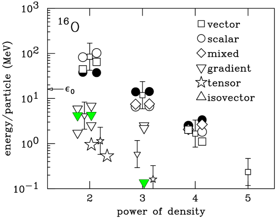
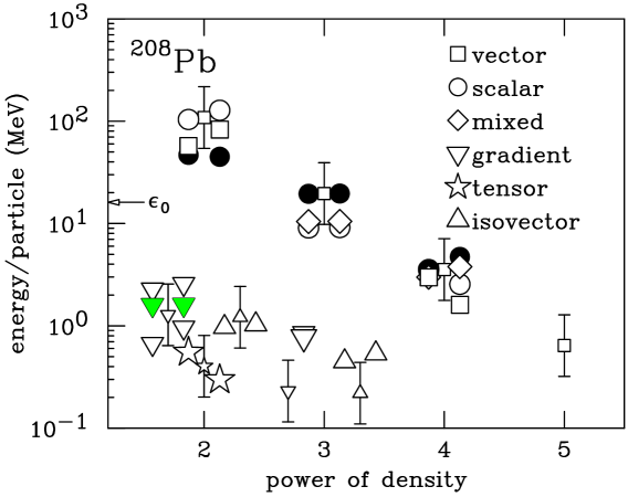
FIG. 1.: Contributions to the energy per particle in ¹⁶O determined by logarithmic derivatives with respect to the model parameters (see text) for two RMF point-coupling models from Ref. [12]. Absolute values are shown. The filled symbols are net values. The small symbols indicate estimates based on NDA [Eq. (14)], with the error bars corresponding to natural coefficients from 1/2 to 2.

FIG. 2.: Same as Fig. 2 for ²⁰⁸Pb.

The representative RMF models validate the isoscalar estimates from Eq. (14), and the resulting hierarchy of isoscalar contributions is quite clear. The question is: How far down in the hierarchy can we reliably determine contributions and their associated parameters? To address this question, we can consider a series of models truncated at different levels in the hierarchy. As additional terms are added, the reproduction of experimental observables should improve. When improvement stops, contributions beyond this point are unresolved and irrelevant.

To make a meaningful analysis, we must decide on the most relevant observables. The Density Functional Theory (DFT) perspective motivates the observables that we expect to calculate reliably with a RMF model [41]. These include the total binding energy, density distributions at low momentum transfer (including rms radii), the chemical potential, and splittings between quasi-particle levels near the Fermi surface. We construct a measure of the accuracy of the fit to these observables, which is based on squared deviations between predictions and data for various observables but is not a statistical $\chi^{2}$. Instead, we apply relative weightings based on our DFT expectations, with the total energy weighted most heavily. Properties of five doubly magic nuclei were used (see Refs. [11] and [12] for details).

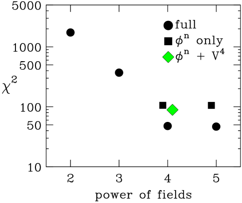
FIG. 3.: Figure of merit (“$\chi^{2}$”) values for RMF meson models [11, 12], ordered according to the truncation level of the energy functional.

In Fig. 3, the impact of different RMF meson model truncations is shown by plotting this figure of merit (“$\chi^{2}$”) against the maximum power of fields in a truncated energy functional. We have performed this test with both point-coupling and meson models, with similar conclusions. We focus here on the meson model results because we are able to directly compare them to standard phenomenological models. (See Ref. [12] for the point-coupling analog.) The “full” models (which include all nonredundant terms at a given order) show that one needs to go to the fourth power of fields to get the best fits, but going further yields no improvement. Analogous behavior is found for RMF point-coupling models with powers of densities replacing powers of fields, although the quality of the fit is much better when the truncation is at the cubic level [12]. Thus contributions to the energy/particle at the level of 1 MeV or so are at the limit of resolution. Fifth-order isoscalar contributions to the energy/particle, which are predicted to be less than 1 MeV, are simply not determined by the optimization [12].

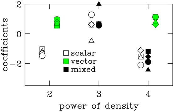
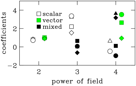
FIG. 4.: Coefficients for four accurately fit RMF point-coupling models from Ref. [12]. Each model is represented by a different shape, and the shading shows the type of term (scalar, vector, or mixed).

FIG. 5.: Coefficients for four accurately fit RMF meson models from Refs. [11] and [42]. Each model is represented by a different shape, and the shading shows the type of term (scalar, vector, or mixed). Several parameter values are slightly beyond the graph limits and so do not appear.

The “$\phi^{n}$ only” results in Fig. 3, which include only scalar fields for $n>2$, show that nearly optimal results can be obtained with just a subset of terms at each order. This explains the successes of the most widely used RMF models, which add only $\phi^{3}$ and $\phi^{4}$ terms to the original Walecka model lagrangian. Since the coefficients are underdetermined by the data, it is not surprising that the systematic optimization of more complete RMF models yields multiple EFT parameter sets with accurate reproductions of nuclear properties [11, 12]. The variation of coefficient values in Eq. (11) provides a measure of how well the parameters are actually determined by the data. In Fig. 5, the seven coefficients of isoscalar, non-gradient terms from four point-coupling models are plotted. The analogous results for coefficients in several meson models is shown in Fig. 5. We note that all coefficients are natural, i.e., order unity. However, the spread in coefficient values is significant, particularly for the meson models, and does not correspond well to the power-counting order. We conclude that different linear combinations of the coefficients must be considered to draw reliable conclusions about how many are determined by the data.

Can we find a more systematic power counting scheme? The similar size of the scalar density $\rho_{{\scriptstyle\rm s}}$ and the vector density $\rho_{{\scriptscriptstyle\rm B}}$ suggests that we count instead powers of $\rho_{+}\equiv(\rho_{{\scriptstyle\rm s}}+\rho_{{\scriptscriptstyle\rm B}})/2$ and $\rho_{-}\equiv(\rho_{{\scriptstyle\rm s}}-\rho_{{\scriptscriptstyle\rm B}})/2$. The corresponding “improved” coefficients are listed in Table I [see Eq. (11)]. The spread in these coefficients for four RMF point-coupling models from Ref. [12] are shown in Fig. 6. The terms are organized according to the power of $\rho_{+}$ and $\rho_{-}$, with $\rho_{-}$ behaving as $\rho_{+}^{8/3}$ [12].

The leading orders are very well determined, with a systematic increase in uncertainty. Even the sign is undetermined for the parameter $\widetilde{\Omega}_{4}$, which is shown with unfilled symbols, but the next parameter ($\widetilde{\Omega}_{6}$) appears to be reasonably well determined. Higher-order terms are undetermined from the optimizations. Deduced values and uncertainties based on this sample of models are given in Table I. We see that of the seven isoscalar, non-gradient parameters in Eq. (11), four linear combinations are clearly determined by bulk nuclear observables, with probably a fifth combination as well.

TABLE I.: Improved coefficients for point-coupling RMF models [12].

coefficient	linear combination	density scaling	deduced value
$\widetilde{\Omega}_{1}$	$\widetilde{\kappa}_{2}+\widetilde{\zeta}_{2}$	$\rho_{+}$	$-0.51\pm 0.01$
$\widetilde{\Omega}_{3}$	$\widetilde{\kappa}_{3}+\widetilde{\eta}_{1}$	$\rho_{+}^{2}$	$+1.3\pm 0.1$
$\widetilde{\Omega}_{2}$	$\widetilde{\kappa}_{2}-\widetilde{\zeta}_{2}$	$\rho_{-}$	$-2.0\pm 0.4$
$\widetilde{\Omega}_{5}$	$\widetilde{\kappa}_{4}+\widetilde{\zeta}_{4}+\widetilde{\eta}_{2}$	$\rho_{+}^{3}$	$-2.4\pm 0.7$
$\widetilde{\Omega}_{4}$	$\widetilde{\kappa}_{3}-\widetilde{\eta}_{1}/3$	$\rho_{+}\rho_{-}$	$+0.2\pm 1.0$
$\widetilde{\Omega}_{6}$	$\widetilde{\kappa}_{4}-\widetilde{\zeta}_{4}$	$\rho_{+}^{2}\rho_{-}$	$-2.6\pm 0.8$
$\widetilde{\Omega}_{7}$	$\widetilde{\kappa}_{4}+\widetilde{\zeta}_{4}-\widetilde{\eta}_{2}2/3$	$\rho_{+}\rho_{-}^{2}$

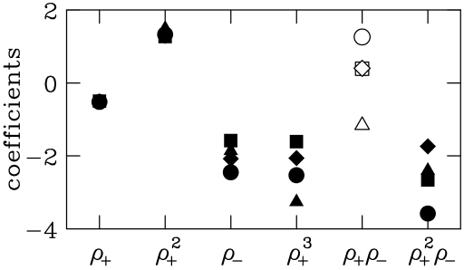
FIG. 6.: Improved coefficients for the same four models as in Fig. 5. The “order” is determined by counting powers of $\rho_{+}$ and $\rho_{-}$.

Now we return to consider a more complete version of Eq. (11) by including the leading isovector and tensor terms:

$$E = \int\!d^{3}x\,\sum_{\alpha}^{\rm occ}\,\overline{\psi}_{\alpha}(-i\beta\mathchoice{{\hbox{\boldmath$\displaystyle\alpha\cdot$}}}{{\hbox{\boldmath$\textstyle\alpha\cdot$}}}{{\hbox{\boldmath$\scriptstyle\alpha\cdot$}}}{{\hbox{\boldmath$\scriptscriptstyle\alpha\cdot$}}}{\mathchoice{{\hbox{\boldmath$\displaystyle\nabla$}}}{{\hbox{\boldmath$\textstyle\nabla$}}}{{\hbox{\boldmath$\scriptstyle\nabla$}}}{{\hbox{\boldmath$\scriptscriptstyle\nabla$}}}}+M)\psi_{\alpha}$$ (19)

$$\quad\hbox{}+f_{\pi}^{2}\Lambda^{2}\int\!d^{3}x\,\bigg{\{}\widetilde{\kappa}_{2}{\widetilde{\rho}_{{\scriptstyle\rm s}}}^{\kern 2.0pt2}-\widetilde{\kappa}_{d}({\widetilde{\mathchoice{{\hbox{\boldmath$\displaystyle\nabla$}}}{{\hbox{\boldmath$\textstyle\nabla$}}}{{\hbox{\boldmath$\scriptstyle\nabla$}}}{{\hbox{\boldmath$\scriptscriptstyle\nabla$}}}}}{\widetilde{\rho}_{{\scriptstyle\rm s}}})^{2}+\widetilde{\kappa}_{3}\widetilde{\rho}_{{\scriptstyle\rm s}}^{\kern 2.0pt3}+\widetilde{\kappa}_{4}\widetilde{\rho}_{{\scriptstyle\rm s}}^{\kern 2.0pt4}+\widetilde{\eta}_{1}\widetilde{\rho}_{{\scriptscriptstyle\rm B}}^{\kern 2.0pt2}\widetilde{\rho}_{{\scriptstyle\rm s}}+\widetilde{\eta}_{2}\widetilde{\rho}_{{\scriptscriptstyle\rm B}}^{\kern 2.0pt2}\widetilde{\rho}_{{\scriptstyle\rm s}}^{\kern 2.0pt2}$$

$$\qquad\qquad\qquad\qquad\hbox{}+\widetilde{\zeta}_{2}\widetilde{\rho}_{{\scriptscriptstyle\rm B}}^{\kern 2.0pt2}-\widetilde{\zeta}_{d}({\widetilde{\mathchoice{{\hbox{\boldmath$\displaystyle\nabla$}}}{{\hbox{\boldmath$\textstyle\nabla$}}}{{\hbox{\boldmath$\scriptstyle\nabla$}}}{{\hbox{\boldmath$\scriptscriptstyle\nabla$}}}}}\widetilde{\rho}_{{\scriptscriptstyle\rm B}})^{2}+\widetilde{\zeta}_{4}\widetilde{\rho}_{{\scriptscriptstyle\rm B}}^{\kern 2.0pt4}-\widetilde{\alpha}_{1}{\widetilde{\rho}_{{\scriptstyle\rm s}}}({\widetilde{\mathchoice{{\hbox{\boldmath$\displaystyle\nabla$}}}{{\hbox{\boldmath$\textstyle\nabla$}}}{{\hbox{\boldmath$\scriptstyle\nabla$}}}{{\hbox{\boldmath$\scriptscriptstyle\nabla$}}}}}{\widetilde{\rho}_{{\scriptstyle\rm s}}})^{2}-\widetilde{\alpha}_{2}{\widetilde{\rho}_{{\scriptstyle\rm s}}}({\widetilde{\mathchoice{{\hbox{\boldmath$\displaystyle\nabla$}}}{{\hbox{\boldmath$\textstyle\nabla$}}}{{\hbox{\boldmath$\scriptstyle\nabla$}}}{{\hbox{\boldmath$\scriptscriptstyle\nabla$}}}}}\widetilde{\rho}_{{\scriptscriptstyle\rm B}})^{2}$$

$$\qquad\qquad\qquad\qquad\hbox{}+\widetilde{\xi}_{2}\widetilde{\rho}_{3}^{\kern 2.0pt2}-{\widetilde{\xi}}_{d}({\widetilde{\mathchoice{{\hbox{\boldmath$\displaystyle\nabla$}}}{{\hbox{\boldmath$\textstyle\nabla$}}}{{\hbox{\boldmath$\scriptstyle\nabla$}}}{{\hbox{\boldmath$\scriptscriptstyle\nabla$}}}}}\widetilde{\rho}_{3})^{2}+\widetilde{\eta}_{\rho}\widetilde{\rho}_{3}^{\kern 2.0pt2}{\widetilde{\rho}_{{\scriptstyle\rm s}}}+\widetilde{f}_{v}{\widetilde{\mathchoice{{\hbox{\boldmath$\displaystyle\nabla$}}}{{\hbox{\boldmath$\textstyle\nabla$}}}{{\hbox{\boldmath$\scriptstyle\nabla$}}}{{\hbox{\boldmath$\scriptscriptstyle\nabla$}}}}}\widetilde{\rho}_{{\scriptscriptstyle\rm B}}\cdot\mathchoice{{\hbox{\boldmath$\displaystyle\widetilde{{s}}$}}}{{\hbox{\boldmath$\textstyle\widetilde{{s}}$}}}{{\hbox{\boldmath$\scriptstyle\widetilde{{s}}$}}}{{\hbox{\boldmath$\scriptscriptstyle\widetilde{{s}}$}}}+\widetilde{f}_{\rho}{\widetilde{\mathchoice{{\hbox{\boldmath$\displaystyle\nabla$}}}{{\hbox{\boldmath$\textstyle\nabla$}}}{{\hbox{\boldmath$\scriptstyle\nabla$}}}{{\hbox{\boldmath$\scriptscriptstyle\nabla$}}}}}\widetilde{\rho}_{3}\cdot\mathchoice{{\hbox{\boldmath$\displaystyle\widetilde{s}_{{\mathchoice{{\hbox{\boldmath$\displaystyle\tau$}}}{{\hbox{\boldmath$\textstyle\tau$}}}{{\hbox{\boldmath$\scriptstyle\tau$}}}{{\hbox{\boldmath$\scriptscriptstyle\tau$}}}}}$}}}{{\hbox{\boldmath$\textstyle\widetilde{s}_{{\mathchoice{{\hbox{\boldmath$\displaystyle\tau$}}}{{\hbox{\boldmath$\textstyle\tau$}}}{{\hbox{\boldmath$\scriptstyle\tau$}}}{{\hbox{\boldmath$\scriptscriptstyle\tau$}}}}}$}}}{{\hbox{\boldmath$\scriptstyle\widetilde{s}_{{\mathchoice{{\hbox{\boldmath$\displaystyle\tau$}}}{{\hbox{\boldmath$\textstyle\tau$}}}{{\hbox{\boldmath$\scriptstyle\tau$}}}{{\hbox{\boldmath$\scriptscriptstyle\tau$}}}}}$}}}{{\hbox{\boldmath$\scriptscriptstyle\widetilde{s}_{{\mathchoice{{\hbox{\boldmath$\displaystyle\tau$}}}{{\hbox{\boldmath$\textstyle\tau$}}}{{\hbox{\boldmath$\scriptstyle\tau$}}}{{\hbox{\boldmath$\scriptscriptstyle\tau$}}}}}$}}}$$

$$\qquad\qquad\qquad\qquad\hbox{}+\mbox{electromagnetic terms}+\mbox{higher order terms}\bigg{\}}\ .$$

We will need estimates for isovector, gradient, and tensor densities. An estimate for the isovector density is obtained by a simple scaling of the local-density approximation to the baryon density:

$$\widetilde{\rho}_{3}\longrightarrow{(Z-N)\over 2A}{\langle\rho_{{\scriptscriptstyle\rm B}}\rangle\over f_{\pi}^{2}\Lambda}\ ,$$ (20)

which reproduces the direct average of isovector densities in best-fit models to about 10% accuracy. We use [see Eq. (13)]

$$(\widetilde{\mathchoice{{\hbox{\boldmath$\displaystyle\nabla$}}}{{\hbox{\boldmath$\textstyle\nabla$}}}{{\hbox{\boldmath$\scriptstyle\nabla$}}}{{\hbox{\boldmath$\scriptscriptstyle\nabla$}}}}\widetilde{\rho}_{{\scriptstyle\rm s}})^{2},(\widetilde{\mathchoice{{\hbox{\boldmath$\displaystyle\nabla$}}}{{\hbox{\boldmath$\textstyle\nabla$}}}{{\hbox{\boldmath$\scriptstyle\nabla$}}}{{\hbox{\boldmath$\scriptscriptstyle\nabla$}}}}\widetilde{\rho}_{{\scriptscriptstyle\rm B}})^{2}\longrightarrow{\langle({\mathchoice{{\hbox{\boldmath$\displaystyle\nabla$}}}{{\hbox{\boldmath$\textstyle\nabla$}}}{{\hbox{\boldmath$\scriptstyle\nabla$}}}{{\hbox{\boldmath$\scriptscriptstyle\nabla$}}}}\rho_{{\scriptscriptstyle\rm B}})^{2}\rangle\over f_{\pi}^{4}\Lambda^{4}}$$ (21)

for gradients and

$$\widetilde{\mathchoice{{\hbox{\boldmath$\displaystyle s$}}}{{\hbox{\boldmath$\textstyle s$}}}{{\hbox{\boldmath$\scriptstyle s$}}}{{\hbox{\boldmath$\scriptscriptstyle s$}}}}\longrightarrow{\langle{\mathchoice{{\hbox{\boldmath$\displaystyle s$}}}{{\hbox{\boldmath$\textstyle s$}}}{{\hbox{\boldmath$\scriptstyle s$}}}{{\hbox{\boldmath$\scriptscriptstyle s$}}}}\rangle\over f_{\pi}^{2}\Lambda}$$ (22)

for tensor terms.

Estimates for all of the terms in Eq. (19) and the corresponding contributions from the two point-coupling models are indicated with different small symbols in Figs. 2 (¹⁶O) and 2 (²⁰⁸Pb). Solid inverted triangles represent the net contribution of two gradient terms at second and third order in the density expansion. The actual contributions from the direct fits for the two nuclei from isovector, gradient, and tensor terms exhibit significant differences, but the estimates follow these systematics quite reasonably. This enables us to predict how many parameters of each type can be determined reliably.

The isovector terms appear only on the graphs for ²⁰⁸Pb. The factor $(N-Z)/2A$, which is only 10% even for Pb, severely cuts down the sensitivity to isovector terms (especially since the factor must appear with even powers). The magnitude of the leading isovector term ($\propto\widetilde{\xi}_{2}\widetilde{\rho}_{3}^{2}\,$) is comparable to the fourth-order isoscalar term, which is at the limit of what can be determined reliably from fitting the binding energy. Fits of the subleading term ($\propto\widetilde{\eta}_{\rho}\widetilde{\rho}_{{\scriptstyle\rm s}}\widetilde{\rho}_{3}^{2}$) are borderline unnatural, which is typical for energy contributions that are essentially unresolved. Furthermore, while individual values for $\widetilde{\xi}_{2}$ and $\widetilde{\eta}_{\rho}$ vary widely between different parameter sets, the combination $\widetilde{\xi}_{2}+\widetilde{\eta}_{\rho}\langle\widetilde{\rho}_{{\scriptstyle\rm s}}\rangle$, with $\langle\widetilde{\rho}_{{\scriptstyle\rm s}}\rangle\approx\langle\widetilde{\rho}_{{\scriptscriptstyle\rm B}}\rangle\approx 0.16$ from averaging over nuclei from oxygen to lead, is well determined. We conclude that only one isovector parameter is determined by the bulk observables. A term proportional to $(\widetilde{\rho}_{3})^{4}$, which one might think important for the neutron-star equation of state, is completely undetermined by ordinary nuclei. Our results support previous observations in meson models that at the mean-field level, the role of the $\rho$ meson is simply to reproduce the correct symmetry energy [44, 43]. Including any other isovector degrees of freedom, such as an isovector, scalar meson, is unnecessary. However, the use of specific isovector observables, such as the difference between neutron and proton distributions at low momentum transfer, may provide more constraints on the isovector parameters.

The energy estimates for isoscalar tensor terms imply that only one parameter, at best, can be determined. Higher-spin terms, which will require more gradients and have smaller average densities, are not at all constrained. The tensor terms are interesting to consider because a fraction of the spin-orbit force can be generated by including an isoscalar tensor coupling of the vector field to the nucleon. At the same time, the scalar and vector fields will be reduced (and therefore the effective nucleon mass $M^{\ast}$ will be increased). Nevertheless, the spin-orbit potential arises predominantly from the large scalar and vector fields; attributing more than one-third of the potential to the tensor coupling produces unrealistic surface systematics [45]. In Ref. [46], it was shown how to accurately relate the size of the tensor coupling to the value of $M^{\ast}$ in nuclear matter and the size of spin-orbit splittings in finite nuclei.

Finally, the gradient terms follow the same pattern in the energy: the leading term is barely above the limit of resolution. In fact, there are two isoscalar gradient terms at leading order (scalar and vector), but if we consider linear combinations based on $\rho_{+}$ and $\rho_{-}$ (see the improved coefficients $\widetilde{\Delta}_{i}$ and $\widetilde{A}_{i}$ in [12]), only their sum is well determined. The subleading-order contributions appear to be highly unnatural individually, but their sum almost vanishes. Thus we conclude that only one gradient parameter is determined. This has implications for the possibility of resolving effective meson masses from fits of point-coupling parameters. In particular, estimates for the scalar and vector masses squared are $\Lambda^{2}\widetilde{\kappa}_{2}/\widetilde{\kappa}_{d}$ and $\Lambda^{2}\widetilde{\zeta}_{2}/\widetilde{\zeta}_{d}$, respectively. Since $\widetilde{\kappa}_{d}$ and $\widetilde{\zeta}_{d}$ are not individually determined, only the difference of the inverse squared masses can be extracted.

III Implications and Summary

We have shown that EFT power counting and naturalness lead to reliable estimates of the energy contribution in a finite nucleus from any term in a general RMF energy functional. By examining energy systematics based on these estimates and the spread among coefficient values in models fit to a given set of nuclear observables, we can deduce how many parameters are actually constrained by those data. We conclude that four (possibly five) isoscalar, non-gradient parameters, one gradient parameter, and one isovector parameter are well determined by the usual bulk nuclear observables (binding energies, charge density distributions, and spin-orbit splittings in doubly magic nuclei). Since conventional RMF models include this distribution of parameters (plus two additional unnecessary gradient terms), it is not surprising that empirical surveys have found no phenomenological reason to add additional terms [6].

The handful of parameters that are well determined can be associated with an equal number of nuclear properties and general features of RMF models. In particular,

1. Two isoscalar, non-gradient parameters are very well determined. These correspond to the highly constrained values for the equilibrium density ($k_{{\scriptscriptstyle\rm F}}\approx 1.30\pm 0.01\,\mbox{fm}^{-1}$) and binding energy ($16.0\pm 0.1\,\mbox{MeV}$) of observed nuclear matter.

2. An additional isoscalar constraint is that $M^{\ast}\approx 0.61\pm 0.03$, if the isoscalar tensor term is set to zero. This range ensures an accurate reproduction of spin-orbit splittings in finite nuclei. Small increases in $M^{\ast}$ without changing the splittings can be accommodated by including an isoscalar tensor term, with the trade-off given by a simple local-density approximation in Ref. [46].

3. A fourth isoscalar constraint comes from the nuclear matter compressibility. The constraint is much weaker, in the range of $K\approx 250\pm 50\,$MeV.

4. The possibility of a fifth isoscalar constraint has been considered by Gmuca [25], who argued that one needed separate scalar and vector fourth-order terms to tune the density dependence of the scalar and vector parts of the baryon self-energies. This would correspond to constraining $\widetilde{\Omega}_{6}$ from Table I. In addition, some form of isoscalar nonlinear vector coupling is needed to soften the high-density equation of state to be consistent with observed neutron star masses [43].

5. Since only one isoscalar gradient parameter is determined, it is not useful to allow the scalar and vector masses (or their equivalents in a point-coupling model) to vary independently. Thus it is convenient to fix the vector mass at a natural size, such as the experimental mass for the $\omega$. Then a scalar mass of $500\pm 20\,$MeV is required. (It may be fine tuned using the ⁴⁰Ca rms charge radius 3.45 fm as a target.)

6. The one isovector parameter can be fixed by the surface-corrected volume symmetry energy [40], which falls in the range $34\pm 4\,$MeV [5]. Since no isovector gradient is determined, setting the isovector vector meson mass to the experimental $\rho$ meson mass is adequate.

To produce the best quantitative fits to nuclear properties for any given model, the model parameters should be obtained from an optimization procedure involving calculations of a set of finite nuclei from oxygen to lead [10, 12]. However, to ensure a reasonable (if not optimal) reproduction of finite nuclei, it is sufficient to reproduce the nuclear matter properties given above. Note that all properties must be satisfied and the resulting parameters must be natural.

This last point has important implications for an alternative class of RMF investigations, which are not based on EFT but are defined by some specific underlying physics. Examples include models that contain different degrees of freedom (quarks) [47, 48], or different types of meson–baryon couplings (derivative couplings) [49, 50], or explicit inclusion of chiral symmetry [51, 52, 53, 54, 55, 56]. (The chronology for this development can be gleaned from some recent review articles [2, 3, 4], the papers cited above, and references therein.) Unfortunately, in many of these studies it was believed to be sufficient to reproduce just the nuclear matter equilibrium point, and thus the results for finite nuclei were not as accurate as expected from the EFT analysis [9, 46]. One cannot justify the underlying physics of a model if it can reproduce only a subset of the nuclear calibration data.

Moreover, both the input observables and the parameters are highly correlated and noisy; therefore, it is inappropriate to use the deduced parameters from Table I instead of a direct fit to observables. It is possible to achieve a sensible picture of nuclei by this procedure but not a very accurate fit.

The improved coefficients from Table I suggest that a nonrelativistic point-coupling EFT, with an expansion in $\rho_{{\scriptscriptstyle\rm B}}$ only, should be consistent with similar power-counting estimates. Indeed, the phenomenologically successful Skyrme models are in this category, and an NDA study shows that they are natural [57]. A scale of $\Lambda=600\,$MeV is consistent with the trends in all of the relativistic and nonrelativistic models. A comparison of these approaches from the EFT perspective will be given elsewhere.

The EFT/DFT perspective provides insight into which additional observables might further constrain the parameters of a general RMF functional. Since four or five isoscalar, non-gradient terms in the energy functional are determined, it is unlikely that additional bulk, isoscalar observables will provide further constraints. This is consistent with calculations of deformed even-even nuclei, which reproduce experimental systematics once the energy functional is constrained to reproduce bulk properties of doubly magic nuclei. On the other hand, since only one isovector parameter is fixed, additional isovector observables could be relevant. In particular, an accurate measurement of the neutron radius in a heavy nucleus, which would result from proposed parity violation experiments, may fix an additional isovector parameter. Additional constraints on gradient terms might be provided from data on ground-state currents at nonzero (but low) momentum transfer, for example, from elastic magnetic scattering. An assessment of these constraints within the framework described here is in progress.

- [1] L. I. Schiff, Phys. Rev. 84 (1951) 1, 10.
- [2] B. D. Serot and J. D. Walecka, Adv. Nucl. Phys. 16 (1986) 1.
- [3] B. D. Serot, Rep. Prog. Phys. 55 (1992) 1855.
- [4] B. D. Serot and J. D. Walecka, Int. J. Mod. Phys. E6 (1997) 515.
- [5] C. J. Horowitz and B. D. Serot, Nucl. Phys. A368 (1981) 503.
- [6] P.-G. Reinhard, M. Rufa, J. A. Maruhn, W. Greiner, and J. Friedrich, Z. Phys. A323 (1986) 13.
- [7] M. Rufa, P.-G. Reinhard, J. A. Maruhn, W. Greiner, and M. R. Strayer, Phys. Rev. C38 (1988) 390.
- [8] A. R. Bodmer, Nucl. Phys. A526 (1991) 703.
- [9] R. J. Furnstahl and B. D. Serot, Phys. Rev. C47 (1993) 2338; Phys. Lett. B316 (1993) 12.
- [10] R. J. Furnstahl, B. D. Serot, and H.-B. Tang, Nucl. Phys. A598 (1996) 539.
- [11] R. J. Furnstahl, B. D. Serot, and H.-B. Tang, Nucl. Phys. A615 (1997) 441.
- [12] John J. Rusnak and R. J. Furnstahl, Nucl. Phys. A627 (1997) 495.
- [13] J. D. Walecka, Ann. Phys. (N.Y.) 83 (1974) 491.
- [14] B. D. Serot, Phys. Lett. 86B (1979) 146; 87B (1979) 403 (E).
- [15] L. D. Miller, Phys. Rev. C9 (1974) 537.
- [16] R. Brockmann, Phys. Rev. C18 (1978) 1510.
- [17] L. N. Savushkin, Sov. J. Nucl. Phys. 30 (1979) 340.
- [18] J. Boguta and A. R. Bodmer, Nucl. Phys. A292 (1977) 413.
- [19] A. Bouyssy, S. Marcos, J. F. Mathiot, Nucl. Phys. A415 (1984) 497.
- [20] R. J. Furnstahl, C. E. Price, and G. E. Walker, Phys. Rev. C36 (1987) 2590.
- [21] P.-G. Reinhard, Rep. Prog. Phys. 52 (1989) 439.
- [22] Y. K. Gambhir, P. Ring, and A. Thimet, Ann. Phys. (N.Y.) 198 (1990) 132.
- [23] M. M. Sharma, M. A. Nagarajan, and P. Ring, Ann. Phys. (N.Y.) 231 (1994) 110.
- [24] J. P. Maharana, L. S. Warrier, and Y. K. Gambhir, Ann. Phys. (N.Y.) 250 (1996) 237.
- [25] S. Gmuca, Z. Phys. A342 (1992) 387; Nucl. Phys. A547 (1992) 447.
- [26] R. J. Furnstahl and B. D. Serot, Proc. Particles and Nuclear International Conference 1999, Uppsala, Sweden, e-print nucl-th/9907073.
- [27] B. A. Nikolaus, T. Hoch, D. G. Madland, Phys. Rev. C46, 1757 (1997).
- [28] J. L. Friar, D. G. Madland, and B. W. Lynn, Phys. Rev. C53, 3085 (1996).
- [29] R. M. Dreizler and E. K. U. Gross, Density Functional Theory (Springer, Berlin, 1990)
- [30] A. Bouyssy, J. F. Mathiot, V. G. Nguyen, S. Marcos, Phys. Rev. C 36 (1987) 380.
- [31] P. G. Blunden and P. McCorquodale, Phys. Rev. C38 (1988) 1861.
- [32] M. R. Anastasio, L. S. Celenza, W. S. Pong, C. M. Shakin, Phys. Rep. 100 (1983) 328.
- [33] C. J. Horowitz and B. D. Serot, Phys. Lett. 137B (1984) 287; Nucl. Phys. A464 (1987) 613; A473 (1987) 760 (E).
- [34] R. Brockmann and R. Machleidt, Phys. Lett. 149B (1984) 283; Phys. Rev. C42 (1990) 1965.
- [35] F. de Jong and R. Malfliet, Phys. Rev. C44 (1991) 998.
- [36] H. Georgi and A. Manohar, Nucl. Phys. B234 (1984) 189.
- [37] J. L. Friar, Few Body Syst. 99 (1996) 1.
- [38] H. Georgi, Weak Interaction and Modern Particle Theory (Benjamin/Cummings, Menlo Park, CA 1984).
- [39] H. Georgi, Phys. Lett. B298 (1993) 187.
- [40] P. A. Seeger and W. M. Howard, Nucl. Phys. A238 (1975) 491.
- [41] W. Kohn and L. J. Sham, Phys. Rev. A140 (1965) 1133.
- [42] J. J. Rusnak, Ph.D. thesis, Ohio State University, 1997.
- [43] H. Mueller and B. D. Serot, Nucl. Phys. A606 (1996) 508.
- [44] C. J. Horowitz and B. D. Serot, Nucl. Phys. A399 (1983) 529.
- [45] G. Hua, T. v. Chossy, and W. Stocker, Phys. Rev. C60 (1999), in press.
- [46] R. J. Furnstahl, J. J. Rusnak, and B. D. Serot, Nucl. Phys. A632 (1998) 607.
- [47] K. Saito and A.W. Thomas, Phys. Lett. B327 (1994) 9.
- [48] K. Saito, K. Tsushima, A. W. Thomas, Nucl. Phys. A609 (1996) 339.
- [49] J. Zimanyi and S. A. Moskowski, Phys. Rev. C42 (1990) 1416.
- [50] M. Chiapparini, A. Delfino, M. Malheiro, and A. Gattone, Z. Phys. A357 (1997) 47.
- [51] A. K. Kerman and L. D. Miller, in Second High-Energy Heavy Ion Summer Study, Lawrence Berkeley Laboratory report LBL–3675 (1974).
- [52] B. L. Birbrair, V. N. Fomenko, and L. N. Savushkin, J. Phys. G8 (1982) 1517.
- [53] J. Boguta, Phys. Lett. 120B (1983) 34; 128B (1983) 19.
- [54] S. Sarkar and S. K. Chowdhury, Phys. Lett. 153B (1985) 358.
- [55] E. K. Heide, S. Rudaz, and P. J. Ellis, Nucl. Phys. A571 (1994) 713.
- [56] G. Carter, P. J. Ellis, and S. Rudaz, Nucl. Phys. A603 (1996) 367.
- [57] R. J. Furnstahl and J.C. Hackworth, Phys. Rev. C 56 (1997) 2875.