Dynamical restriction for a growing neck due to mass parameters in a dinuclear system

Abstract

Mass parameters for collective variables of a dinuclear system and strongly deformed mononucleus are microscopically formulated with the linear response theory making use of the width of single particle states and the fluctuation–dissipation theorem. For the relative motion of the nuclei and for the degree of freedom describing the neck between the nuclei, we calculate mass parameters with basis states of the adiabatic and diabatic two-center shell model. Microscopical mass parameters are found larger than the ones obtained with the hydrodynamical model and give a strong hindrance for a melting of the dinuclear system along the internuclear distance into a compound system. Therefore, the dinuclear system lives a long time enough comparable to the reaction time for fusion by nucleon transfer. Consequences of this effect for the complete fusion process are discussed.

I Introduction

The synthesis of transuranium and superheavy elements, the production of superdeformed nuclei and nuclei far from the line of stability stimulate the study of phenomena of complete fusion in heavy ion collisions at energies less than 15 MeV/nucleon. The fusion of heavy ions is characterized by the formation of a dinuclear system (DNS) at the initial stage of reaction when a significant part of the kinetic energy is transferred into excitation energy. In that case one has to describe the evolution of the DNS and strongly deformed nucleus by collective coordinates $Q$, namely by the distance $R$ between the centers of colliding nuclei (or relative elongation $\lambda$ of the system), the mass and charge asymmetry degrees of freedom $\eta=(A_{1}-A_{2})/A$ and $\eta_{Z}=(Z_{1}-Z_{2})/Z$, respectively, ($A_{1}$, $A_{2}$ and $Z_{1}$, $Z_{2}$ are mass and charge numbers of the nuclei, $A=A_{1}+A_{2}$, $Z=Z_{1}+Z_{2}$), the parameter $\varepsilon$ of the neck and deformation coordinates of nuclei [1, 2, 3, 4, 5, 6, 7, 8, 9]. Then dissipative, conservative and inertial forces for collective variables, arising from the nucleus-nucleus interaction, are needed to be determined.

The present fusion models can be distinguished by the choice of the relevant collective variables along which fusion mainly occurs. While many models study the fusion in $R$ at a practically fixed value of $\eta$, the DNS model  [7, 10] considers the DNS evolution in mass asymmetry by nucleon or cluster transfers as the main path to the compound nucleus. The DNS model assumes basically that the neck degree of freedom is fixed in the evolution in $\eta$ and the nuclei are hindered to melt together by a variation in the relative distance. As was shown in Refs. [11, 12, 13, 14] this occurs due to the relatively large inertia of the neck degree of freedom and structural forbiddenness effects. In this paper we study dynamical restrictions for the growth of the neck in the DNS and suggest proper methods of the calculation of the DNS inertia tensor.

There are various macroscopical and microscopical approaches to calculate the inertia tensor [15]. The macroscopical approaches (see, for example, [5, 9]) are based on the hydrodynamical model of the nucleus. A calculation of the inertia tensor with a theory for quantum fluid dynamics is suggested in Ref. [16]. By using a random-matrix model to describe the coupling between a collective nuclear variable and intrinsic degrees of freedom and with the help of the functional integral approach, mass parameters are derived in Ref. [17]. In the linear response theory [18, 19] the inertia tensor is found for fissioning nuclei. The microscopical approaches mainly use the cranking type expression and perform calculations in different single particle bases applying adiabatic [3, 4, 20] or diabatic [21, 22] two-center shell models. Difficulties in the cranking type calculations arise for collective motions with large amplitudes, for example, in fusion or fission, due to pseudo–crossings or crossings of levels in the single particle spectrum. Some publications disregard the contributions from the crossings (pseudo–crossings) which means a neglect of effects of configuration changes on the mass parameters during the evolution of the nuclear shape in spite of the fact that the collective inertia is strongly influenced by level crossings (pseudo–crossings) [23, 24]. In order to overcome this problem, two–body collisions should be regarded which lead to a width of the single particle levels and an effective reduction of the level crossing effects. For example, calculations of the nuclear inertia in a generalized cranking model with pairing correlations yielded masses of about one order of magnitude larger than the ones without pairing [25].

One of the aims of the present paper is to obtain analytical expressions for mass parameters using models and methods which include residual interaction effects. In Sect. 2 the mass parameters are obtained within the linear response theory taking the fluctuation-dissipation theorem and the width of single particle states into account. The same mass parameters are also derived by Fermi’s golden rule and by smoothing the single particle spectrum in the mean–field cranking formula. In Sect. 3 the mass parameters for the relevant collective variables (mass asymmetry, elongation, neck and deformation parameters) of the DNS and strongly deformed nuclear systems are evaluated in the two-center shell model with adiabatic and diabatic bases. Sect. 4 contains a short summary.

II Microscopical inertia

A Derivation from collective response function

Let us consider a nuclear system described by a single collective coordinate $Q$ and intrinsic single particle coordinates $x_{i}$ (with the conjugated momentum $p_{i}$) and assume the following effective Hamiltonian [18]:

$$\hat{H}(x_{i},p_{i},Q) = \hat{H}(x_{i},p_{i},Q_{0})+(Q-Q_{0})\hat{F}(x_{i},p_{i},Q_{0})$$ (1)

$$+ \frac{1}{2}(Q-Q_{0})^{2}<\frac{\partial^{2}\hat{H}(x_{i},p_{i},Q)}{\partial Q^{2}}>_{Q_{0},T_{0}}$$ (2)

The shape of the nuclear mean field is changed with the collective coordinate $Q$ that introduces the coupling between $Q$ and the nucleonic degrees of freedom. Eq. (1) is obtained by expanding the Hamiltonian to second order in the vicinity of $Q_{0}$ and by approximating the second order term in a kind of unperturbed limit. The coupling term between the collective and intrinsic motion is proportional to the first order in $\delta Q=Q-Q_{0}$ with an operator $\hat{F}$ given by the derivative of the mean field with respect to $Q$ in the neighborhood of $Q_{0}$. In this way global motion is described within a locally harmonic approximation.

By applying the linear response theory [18, 26], the Fourier transform of the collective response function is defined as

$$\chi_{coll}(\omega)=\frac{\chi(\omega)}{1+k\chi(\omega)},$$ (3)

where $\chi(\omega)$ is the Fourier transform of the response function for intrinsic motion and measures how, at some given $Q_{0}$ and temperature $T_{0}$, the nucleonic degrees of freedom react to the coupling term $\hat{F}\delta Q$. The coupling constant $k$ is written in the form

$$-k^{-1}=<\frac{\partial^{2}\hat{H}(x_{i},p_{i},Q)}{\partial Q^{2}}>_{Q_{0},T_{0}}=\frac{\partial^{2}E(Q,S_{0})}{\partial Q^{2}}|_{Q_{0}}+\chi(\omega=0)=C(0)+\chi(0)$$ (4)

with $\chi(0)$ and $C(0)$ being the static response and stiffness, respectively. Since the constant $k$ is entirely determined by quasi-static properties, it is no surprise that $E$ is the internal energy at a given entropy $S_{0}$ or the free energy at a given temperature $T_{0}$. The structure of Eq.(2) reflects self–consistency between the treatment of collective and microscopic dynamics. It expresses the response of the system of interacting nucleons in terms of the response of the individual nucleons.

The local motion in the $Q$ variable is described in terms of the collective response function $\chi_{coll}$. A short calculation leads to the following approximation for the mass coefficient [18, 19, 26, 27]:

$$M=-\frac{1}{2k^{2}}\frac{\partial^{2}(\chi_{coll}(\omega))^{-1}}{\partial\omega^{2}}|_{\omega=0}=(1+\frac{C(0)}{\chi(0)})^{2}[M^{cr}+\frac{\gamma^{2}(0)}{\chi(0)}],$$ (5)

where

$$M^{cr}=\frac{1}{2}\frac{\partial^{2}\chi(\omega)}{\partial\omega^{2}}|_{\omega=0}$$ (6)

is the inertia in the zero-frequency limit of the second derivative of the intrinsic response function. $M^{cr}$ can be shown to be similar to the one of the cranking model. For many applications, the value of $C(0)/\chi(0)$ is much less than unity. The additional term $\gamma^{2}(0)/\chi(0)$ in Eq. (4) gives a positive contribution to $M$ where $\gamma(0)$ is the friction coefficient defined by

$$\gamma(0)=-i\frac{\partial\chi(\omega)}{\partial\omega}|_{\omega=0}=\frac{\partial\chi^{{}^{\prime\prime}}(\omega)}{\partial\omega}|_{\omega=0}=\frac{1}{2T_{0}}\psi^{{}^{\prime\prime}}(0).$$ (7)

The dissipative part of the response function $\chi^{{}^{\prime\prime}}(\omega)$ is connected with the dissipative part of the correlation function $\psi^{{}^{\prime\prime}}(\omega)$ through the fluctuation-dissipation theorem:

$$\chi^{{}^{\prime\prime}}(\omega)=\frac{1}{\hbar}\tanh(\frac{\hbar\omega}{2T_{0}})\psi^{{}^{\prime\prime}}(\omega).$$ (8)

The $\psi^{{}^{\prime\prime}}(\omega)$ has a singularity of $\delta$–function type at $\omega=0$:

$$\psi^{{}^{\prime\prime}}(\omega)=2\pi\psi^{0}\delta(\omega)+\psi^{{}^{\prime\prime}}_{R}(\omega)$$ (9)

with $\psi^{{}^{\prime\prime}}_{R}(\omega)$ being regular at $\omega=0$. In the case of an independent particle model we have

$$\psi^{{}^{\prime\prime}}(\omega)=\pi\hbar\sum_{j,k}|F_{jk}|^{2}n(e_{j})[1-n(e_{k})][\delta(\hbar\omega-e_{kj})+\delta(\hbar\omega+e_{kj})].$$ (10)

Here, $e_{kj}=e_{k}-e_{j}$ is the difference of single particle energies, $n(e_{j})$ are the occupation numbers and $F_{jk}=<j|\hat{F}|k>$ the single particle matrix elements of the operator $\hat{F}$. At $j=k$ and $\omega=0$ we find the contributions from the diagonal matrix elements:

$$\psi^{0}=\sum_{k}|F_{kk}|^{2}n(e_{k})[1-n(e_{k})]=T_{0}\sum_{k}\left|\frac{\partial n(e)}{\partial e}\right|_{e=e_{k}}\left(\frac{\partial e_{k}}{\partial Q}\right)^{2}.$$ (11)

The last part in (11) was derived with a Fermi distribution for the occupation numbers, which is characterized by the temperature $T_{0}$. The value of $T_{0}$ does not effectively go to zero with decreasing excitation energy because each single particle level has a width due to the two-body interaction. Indeed at zero excitation energy the distribution of the occupation numbers deviates from a step function at least due to pairing correlations. If we replace the $\delta$–functions in Eq.(8) or (9), we have to apply a Lorentzian functions with the double single particle width $2\Gamma$ where $\Gamma$ is the single particle width, because $\hbar\omega$ is the transition energy between two single particle states [18]. Therefore, we substitute the $\delta-$functions in Eq. (9) by $\Gamma/[\pi((\hbar\omega\pm e_{kj})^{2}+\Gamma^{2})]$. Then using Eqs. (6)-(10), we can write the friction coefficient in the following form:

$$\gamma(0)=\gamma^{diag}(0)+\gamma^{nondiag}(0),$$ (12)

where

$$\gamma^{diag}(0)=\frac{\hbar}{\Gamma}\sum_{k}\left|\frac{\partial n(e)}{\partial e}\right|_{e=e_{k}}\left(\frac{\partial e_{k}}{\partial Q}\right)^{2}.$$ (13)

For smaller temperatures $T_{0}<2$ MeV which are of interest here, $\gamma^{diag}(0)$ is much larger than $\gamma^{nondiag}(0)$ [18]. The static response is found as

$$\chi(0)=\lim_{\epsilon\to 0}\int\limits_{-\infty}^{+\infty}\frac{d\omega}{\pi}\frac{\chi^{{}^{\prime\prime}}(\omega)}{\omega-i\epsilon}=\lim_{\epsilon\to 0}\int\limits_{-\infty}^{+\infty}\frac{d\omega}{\hbar\pi}\frac{\tanh(\frac{\hbar\omega}{2T_{0}})\psi^{{}^{\prime\prime}}(\omega)}{\omega-i\epsilon}=\chi^{diag}(0)+\chi^{nondiag}(0),$$ (14)

where

$$\chi^{diag}(0)=\sum_{k}\left|\frac{\partial n(e)}{\partial e}\right|_{e=e_{k}}\left(\frac{\partial e_{k}}{\partial Q}\right)^{2}.$$ (15)

With realistic assumptions $\gamma^{diag}(0)\gg\gamma^{nondiag}(0)$ and $\chi^{diag}(0)\gg\chi^{nondiag}(0)$ and neglecting $C(0)/\chi(0)$, we can divide the mass parameter (4) as

$$M=M^{diag}+M^{nondiag}.$$ (16)

The contribution of the diagonal matrix elements of $\hat{F}$ to $M$ are

$$M^{diag}=\frac{(\gamma^{diag}(0))^{2}}{\chi^{diag}(0)}=\frac{\hbar^{2}}{\Gamma^{2}}\sum_{k}\left|\frac{\partial n(e)}{\partial e}\right|_{e=e_{k}}\left(\frac{\partial e_{k}}{\partial Q}\right)^{2}.$$ (17)

If the single particle widths are properly taken into account, the nondiagonal contributions to the inertia are [20]

$$M^{nondiag}=M^{cr}=\hbar^{2}\sum_{k\neq k^{\prime}}\frac{|F_{kk^{\prime}}|^{2}}{e^{2}_{kk^{\prime}}+\Gamma^{2}}\frac{n(e_{k})-n(e_{k^{\prime}})}{e_{k^{\prime}}-e_{k}}.$$ (18)

The main contribution to $M$ is the diagonal part $M^{diag}$ because it dominates for collective variables which are responsible for changes of the nuclear shape of the system [23, 24, 28]. Note that the calculation of $M^{diag}$ is simpler than $M^{nondiag}$. For the case that the pairing residual interaction is regarded and only diagonal matrix elements in the cranking formula are taken into account, Eq. (17) was obtained with $\Gamma=\Delta$ ($\Delta$ is the pairing gap) in Ref. [1, 25]. Starting with an equation for the single particle density matrix extended with an approximate incorporation of particle collisions in the relaxation time approach, the authors of Ref. [29] derived an expression similar to (17) (with $\Gamma=\hbar/\tau$, $\tau$ is the relaxation time) but with a negative sign. This negative sign arises from the fact that the condition of self-consistency between collective and nucleonic dynamics was disregarded in  [29] which is important for a correct calculation of the mass parameters. It was stressed in [18, 30] that within the linear response theory the diagonal component of the friction parameter originates from the ”heat pole” of the correlation function and vanishes when the system is ergodic. As shown in Ref. [31], the well necked DNS-type configurations are not ergodic and stable against chaos. Even at zero excitation energy the level crossings at the Fermi surface lead to considerable mass flow [23, 24, 28] and the diagonal component of the correlation function (or mass parameter) does not vanish.

Besides the mass and friction coefficients, the diffusion coefficients $D_{kl}$ $(k,l=(Q,P))$ must also have a component diagonal in the matrix elements of $\hat{F}$ because they are connected with correlation functions. For example, the diffusion coefficient in momentum is defined as:

$$D_{PP}=\frac{1}{2}\psi^{{}^{\prime\prime}}(\omega=0)=T_{0}\gamma(0).$$ (19)

B Derivation from Fermi’s golden rule

By setting $\hat{H}_{I}=(Q-Q_{0})\hat{F}(x_{i},p_{i},Q_{0})$ as perturbation (see Eq. (1)), the decay rate of a collective state $|n>$ with energy $E_{n}$ to the collective state $|m>$ with energy $E_{m}$ is given in lowest order according to Fermi’s golden rule:

$$w(n\to m+\hbar\omega) = \frac{2\pi}{\hbar}|<m|Q-Q_{0}|n>|^{2}$$ (20)

$$\times \int\limits d(\hbar\omega)|<\hbar\omega|\hat{F}|0>|^{2}\delta(E_{n}-E_{m}-\hbar\omega)\rho_{qs}(\hbar\omega).$$ (21)

Here, the integral is taken over the final states of the intrinsic system with the density $\rho_{qs}$. With the fluctuation-dissipation theorem for small temperatures we have [32]:

$$|<\hbar\omega|\hat{F}|0>|^{2}\rho_{qs}(\hbar\omega)d(\hbar\omega)=\frac{2}{\pi}\frac{\hbar\omega}{2}R(\omega)d\omega$$ (22)

with the relaxation function $R(\omega)={\chi^{{}^{\prime\prime}}(\omega)}/{\omega}$. The half-decay width is obtained from Eq.(21) as

$$\Gamma_{n}=\hbar\sum_{m}w(n\to m+\hbar\omega).$$ (23)

Using the properties of the response function and a Taylor expansion

$$R(\omega)=\frac{\chi^{{}^{\prime\prime}}(\omega)}{\omega}=\frac{1}{\omega}\left[\chi^{{}^{\prime\prime}}(\omega=0)+\left.\frac{\partial\chi^{{}^{\prime\prime}}(\omega)}{\partial\omega}\right|_{\omega=0}\,\omega+\left.\frac{1}{2}\frac{\partial^{2}\chi^{{}^{\prime\prime}}(\omega)}{\partial\omega^{2}}\right|_{\omega=0}\,\omega^{2}+...\right],$$ (24)

and the standard formula for mass $M$ ($E_{n}\neq E_{m}$)

$$M=\frac{\hbar^{2}}{2}(\sum_{m}|<m|Q-Q_{0}|n>|^{2}[E_{n}-E_{m}])^{-1}$$ (25)

we obtain by setting $\Gamma=\Gamma_{n}$ with Eqs. (21)–(25)

$$M=\frac{\hbar}{\Gamma}\frac{\partial\chi^{{}^{\prime\prime}}(\omega)}{\partial\omega}|_{\omega=0}=\frac{\hbar}{\Gamma}\gamma(0).$$ (26)

Large temperatures in (19) effectively lead to a temperature dependence of $\Gamma$ in (26). Since $\gamma(0)$ in Eq. (11) contains the terms with the diagonal matrix elements of the operator $\hat{F}$, the mass parameter $M$ also has the diagonal component $M^{diag}$ (17). So, the contributions to the mass parameter can be again classified as those with diagonal and nondiagonal matrix elements, respectively.

That the mass parameter is proportional to the friction coefficient (see Eq. (26)), has an analogy in the hydrodynamic model. For multipole moments $\lambda$ of the nucleus with $\lambda>1$, the following ratio in the limit of an irrotational flow was derived in [33]

$$M^{irr}_{\lambda}/\gamma^{irr}_{\lambda}=\frac{3A^{2/3}}{8\pi(2\lambda+1)(\lambda-1)r_{0}}\frac{1}{\nu},$$

where $\nu$ is the coefficient of the two-body viscosity and $r_{0}=1.2$ fm.

C Derivation from the mean–field cranking formula

Using the single particle spectrum and the corresponding wave functions, one can obtain the mass parameter with the cranking formula

$$M^{cr}=\hbar^{2}\sum_{\alpha\neq\beta}|<\alpha|\frac{\partial}{\partial Q}|\beta>|^{2}\frac{n(e_{\alpha})-n(e_{\beta})}{e_{\beta}-e_{\alpha}}.$$ (27)

In reality the Hamiltonian of the system contains a residual two-body interaction between the nucleons in addition to the mean field. The residual coupling distributes the strength of single particle states over more complicated states. This spectral smoothing causes the effect that the sum over $\alpha$ and $\beta$ appearing in (27) also includes diagonal terms with $\alpha=\beta$. Let us prove this statement.

The Eq.(27) can be rewritten as

$$M^{cr}=\hbar^{2}\sum_{\alpha\neq\beta}\int\limits de_{1}\delta(e_{1}-e_{\alpha})\int\limits de_{2}\delta(e_{2}-e_{\beta})|<e_{1}|\frac{\partial}{\partial Q}|e_{2}>|^{2}\frac{n(e_{1})-n(e_{2})}{e_{2}-e_{1}}.$$ (28)

Next we use the following replacements

$$\int\limits de_{1}g(e_{1})\to\sum_{k_{1}},\quad\int\limits de_{2}g(e_{2})\to\sum_{k_{2}},$$ (29)

$$\delta(e-e_{k})\to\rho_{k}(e)=\frac{1}{2\pi}\frac{\Gamma}{(e-e_{k})^{2}+(\Gamma/2)^{2}}$$ (30)

and the approximation

$$D^{2}\,|<k_{1}|\frac{\partial}{\partial Q}|k_{2}>|^{2}\approx|F_{k_{1}k_{2}}|^{2}.$$ (31)

Here, $D=1/g$ is average energy distance between single particle states. Then we express the mass (28) as

$$M^{cr}=\frac{\hbar^{2}\Gamma^{2}}{4\pi^{2}}\sum_{\alpha\neq\beta,k_{1},k_{2}}\frac{|F_{k_{1}k_{2}}|^{2}}{[e_{\alpha k_{1}}^{2}+(\Gamma/2)^{2}][e_{\beta k_{2}}^{2}+(\Gamma/2)^{2}]}\frac{n(e_{k_{1}})-n(e_{k_{2}})}{e_{k_{2}}-e_{k_{1}}}.$$ (32)

The energy spreading of the single particle states is taken into account in Eq.(32). A line broadening happens if collisions of particles and holes with the background result in single particle and single hole strength functions that are concentrated around the original single particle energies. The quantity $D\rho_{k}$ determines the average strength function for a particle in state $k$ [34]. In the limit $e_{k_{1}}=e_{k_{2}}=e_{k}$, for $e_{\alpha,\beta}\approx e_{k}$, i.e. when two neighboring levels near the level $k$ are considered, and $8/\pi^{2}\approx 1$, Eq.(32) leads to Eq.(17). Thus, diagonal terms in the mass parameters appear because of the finite width of the single particle levels due to the residual interaction.

III Results of calculations

A Adiabatic two-center shell model

Since in fusion and quasifission we deal with strongly elongated systems, the two-center shell model (TCSM) [3, 4, 11] is appropriate for calculating the potential energy surface. In the TCSM the nuclear shapes are defined by the following set of the coordinates: The elongation $\lambda=l/(2R_{0})$ measuring the length $l$ of the system in units of the diameter $2R_{0}$ of the spherical compound nucleus and used to describe the relative motion, the mass and charge asymmetry coordinates $\eta$ and $\eta_{Z}$, respectively, the neck parameter $\varepsilon=E_{0}/E^{\prime}$ defined by the ratio of the actual barrier height $E_{0}$ to the barrier height $E^{\prime}$ of the two-center oscillator, and the deformation parameters $\beta_{i}=a_{i}/b_{i}$, $i=1,2$, of axially symmetric fragments, defined by the ratio of the semiaxes of the fragments. Since collisions above the Coulomb barrier are discussed, we firstly consider spherical nuclei with $\beta_{i}=1$ and then analyze the deformation effects.

In order to calculate the width of the single particle states, we use the expression [18, 35]

$$\Gamma_{k}=\frac{1}{\Gamma_{0}}\frac{\left(e_{k}-e_{F}\right)^{2}+(\pi T_{0})^{2}}{1+[\left(e_{k}-e_{F}\right)^{2}+(\pi T_{0})^{2}]/c^{2}}.$$ (33)

Here, $e_{F}$ is the Fermi energy. Both parameters $\Gamma_{0}$ and $c$ are known from experience with the optical model potential and the effective masses [18]. Their values are in the following ranges: $0.030\,$MeV${}^{-1}\leq{\Gamma_{0}}^{-1}\leq 0.061\,$MeV^-1, $15\,$MeV$\leq c\leq 30\,$MeV. For small excitations, Eq. (33) is reduced to the expression known in the theory of a Fermi liquid. Since each single particle state has its own width, Eq. (17) is generalized as ($Q_{i}=\lambda,\eta,\eta_{Z},\varepsilon,\beta_{1},\beta_{2}$):

$$M^{diag}_{ij}=\hbar^{2}\sum_{k}\frac{f_{k}}{\Gamma^{2}_{k}}\frac{\partial e_{k}}{\partial Q_{i}}\frac{\partial e_{k}}{\partial Q_{j}}.$$ (34)

For the Fermi occupation numbers $n(e_{k})$, the function

$$f_{k}=-\frac{dn_{k}}{de_{k}}=\frac{1}{4T_{0}}\cosh^{-2}\left(\frac{e_{k}-e_{F}}{2T_{0}}\right)$$ (35)

has a bell-like shape with a width $T_{0}$ and is peaked at the Fermi energy $e_{F}$.

Various calculations of the mass parameter for the motion in $\lambda$ were carried out with expressions similar to Eq. (34), for example in [1,20,25]. When the system adiabatically moves towards the compound nucleus, the value of $M_{\lambda\lambda}$ approximately increases by a factor 10–15 in our and other calculations. In this paper we concentrate on the calculation of the mass parameter $M_{\varepsilon\varepsilon}$ for the motion of the neck to test whether the DNS exists sufficient time enough with a relatively small neck. The dependence of $M_{\varepsilon\varepsilon}$ on $\varepsilon$ is presented in Fig. 1 for the system ¹¹⁰Pd+¹¹⁰Pd at $\lambda=1.6$ which corresponds to the touching configuration in this symmetric reaction. The obtained values of $M_{\varepsilon\varepsilon}$ have the same order of magnitude as in [20] where the pairing correlations were taken into consideration. The value of $M_{\varepsilon\varepsilon}$ increases by a factor 2.5 when the system falls into the fission–type valley [11]. This increase reflects the decrease of the shell correction $\delta U$ with $\varepsilon$ towards $\varepsilon\to 0$. Smaller values of $\delta U$ correspond to larger masses.

In order to obtain the same TCSM potential energy as in the DNS model for the touching configuration, the neck parameter $\varepsilon$ should be set about 0.75 [11]. With this value of $\varepsilon$ the neck radius and the distance between the centers of the nuclei are approximately equal to the corresponding quantities in the DNS.

For the parameter $c$ in Eq. (33) we use the ”standard” value 20 MeV since the masses (31) depend only weakly on this parameter. Setting the parameter $\Gamma^{-1}_{0}=0.045\,$MeV^-1 in (34) and comparing our results with $M^{WW}_{ij}$ obtained in the Werner-Wheeler approximation, we find $M_{\lambda\lambda}=M^{WW}_{\lambda\lambda}$, $M_{\varepsilon\varepsilon}\approx(20-30)M^{WW}_{\varepsilon\varepsilon}$, $M_{\lambda\varepsilon}\approx 0.4M^{WW}_{\lambda\varepsilon}$ and $M_{\lambda\varepsilon}/\sqrt{M_{\lambda\lambda}M_{\varepsilon\varepsilon}}\ll 1$, practically independent of the mass number of the system. Therefore, we can conclude that the microscopical mass parameter of the neck is much larger than the one in the Werner-Wheeler approximation and the nondiagonal component $M_{\lambda\varepsilon}$ is small. Since at the touching configuration the slope of the single-particle levels is small and changes slowly with decreasing elongation, the microscopical mass parameter in $\lambda$ is close to its smooth, hydrodynamical value. In contrast, a large amount of internal reorganization, which occurs at level crossings with decreasing $\varepsilon$, leads to a large neck inertia of the initial DNS. So, the value of $M_{\varepsilon\varepsilon}$ exceeds the mass in the hydrodynamical model due to large values of $|\partial e_{k}/\partial\varepsilon|$. The restriction for the growth of the neck may be understood by analysing the single particle spectrum as a function of $\varepsilon$  [11]. For large $\varepsilon$ and well necked-in shapes, the single particle spectrum shows a good shell structure. The levels show an increasing number of level crossings with increasing $\varepsilon$.

The time-dependence of the neck parameter calculated with the microscopical and Werner-Wheeler mass formulas are compared in the upper part of Fig. 2. The lower part of Fig. 2 shows trajectories in the $(\varepsilon,\lambda)$-plane, calculated with microscopic and Werner-Wheeler masses. An adiabatic potential energy surface is used in all these calculations. Since there are no suitable barriers at smaller values of $\lambda$ and $\varepsilon$ in the adiabatic potential which hinder a growth of the neck, the neck parameter and system length decrease steadily to smaller values, faster in the case with the Werner-Wheeler masses and much slower with the microscopical masses. The experiments on fusion of heavy nuclei can not be explained as a melting with increasing neck together with a decreasing $\lambda$ in an adiabatic potential [11]. It seems that there is an intermediate situation between the adiabatic and diabatic limits. The study of the transition between diabatic and adiabatic regimes gives a potential energy surface which contains quite high barriers for the motion to smaller $\lambda$ and $\varepsilon$ [13, 36]. Therefore, the dynamical calculations with the adiabatic potential energy show a maximal possible growth of the neck. Due to the large moment of inertia in the heavy nuclear system, the dependence of potential energy on the angular momentum in dynamical calculations is disregarded here. Indeed, in fusion reactions with massive nuclei only low angular momenta ($<$ 20 $\hbar$) contribute to the evaporation residue cross section. For the study of fusion, the isotopic composition of the nuclei forming the DNS is chosen with the condition of a $N/Z$-equilibrium in the system with $\eta_{Z}$ following the value of $\eta$ [10]. In processes developing in the shorter times, the coordinate $\eta_{Z}$ could be considered as independent collective variable.

As result of Fig. 2 we find that the microscopical mass parameters keep the system near the entrance configuration for a sufficient long time comparable with the time of reaction even in an adiabatic potential. Therefore, this situation justifies the assumption of a fixed neck as we assume it in the DNS model [7, 10]. When the DNS configuration exists a long time, then thermal fluctuations in the mass asymmetry coordinate play the essential role in the fusion process. Indeed these fluctuations are responsible for the fusion in the DNS model [7, 10]. Thus, the dynamical restriction for the growth of the neck can be caused partly by a large microscopical mass parameter for the neck motion, partly by the potential energy surface intermediate between diabatic and adiabatic limits.

In the adiabatic two-center shell model the mass parameter $M_{\varepsilon\varepsilon}$ slightly increases with the deformation parameters $\beta_{i}$ of the two nuclei in the symmetric system ¹¹⁰Pd+¹¹⁰Pd as shown in Fig. 3. The small variation of $M_{\varepsilon\varepsilon}$ is due to the shell structure. Therefore, the relatively large value of $M_{\varepsilon\varepsilon}$ is a general result for collisions of both spherical and deformed nuclei. Fig. 4 shows the mass parameter $M_{\varepsilon\varepsilon}$ at the touching configuration of symmetric systems $\eta=0$ with $\beta_{i}=1$ as a function of the mass number $A$. The mass $M_{\varepsilon\varepsilon}$ increases with the mass of the system. It slightly decreases with increasing mass asymmetry of the DNS.

B Diabatic two-center shell model

Let us now consider the calculation of the mass parameters (34) with the diabatic single particle energies obtained with the method of maximum-symmetry in the diabatic two-center shell model [22, 36]. In the diabatic motion the nucleons do not occupy the lowest single particle states as in the adiabatic case, but remain in their diabatic states.

Due to the nonzero widths of the single particle states, the distribution of single particle strength over more complicated states is a Lorentzian distribution $\rho_{k}(e)$ as introduced in Eq. (27) instead of the $\delta$-function $\delta(e-e_{k})$ [18]. The occupation number $\widetilde{n}(e_{k})$ of a state $k$ with energy $e_{k}$ and the corresponding value of $\widetilde{f}_{k\text{ }}$ are obtained, respectively, from functions $n(e)$ and $dn(e)/de$ calculated with zero widths of the levels

$$\widetilde{n}(e_{k})=\int n(e)\rho_{k}(e)de,$$ (36)

$$\widetilde{f}_{k}=-\int\frac{dn(e)}{de}\rho_{k}(e)de.$$ (37)

The Lorentzian distribution increases the diffuseness of the Fermi-distribution. The Fermi distribution which is given at the touching configuration of the nuclei in the DNS is destroyed if the further motion of the system runs diabaticly. To treat the diabatic case, we use the following function $n(e)$ for an arbitrary configuration of the system

$$n(e)=\sum_{l=0}^{N}a_{l}\left(\Theta(e-e_{l})-\Theta(e-e_{l+1})\right),$$ (38)

where $\Theta(x)$ is the Heavyside’s function and $e_{l}$ the energy of single particle state $l$ with the occupation number $a_{l}$. Here, the numbers $l=0,...,N$ count the single particle states in the region of the Fermi level. The values $e_{0}$ and $e_{N+1}$ are the low and high limits of the single particle energies. For lower and higher energies, the occupation numbers are one and zero, respectively. Therefore, we assume $a_{0}=1$ and $a_{N}=0$ in (38). The derivative $dn(e)/de$ is expressed as

$$-\frac{dn(e)}{de}=(1-a_{1})\delta(e-e_{1})+\sum_{l=2}^{N-1}(a_{l-1}-a_{l})\delta(e-e_{l})+a_{N-1}\delta(e-e_{N}).$$ (39)

Then we obtain $\widetilde{f}_{k}$ with (37) as follows

$$\widetilde{f}_{k}=(1-a_{1})\rho_{k}(e_{1})+\sum_{l=2}^{N-1}(a_{l-1}-a_{l})\rho_{k}(e_{l})+a_{N-1}\rho_{k}(e_{N}).$$ (40)

In the calculations we assume the same average width for each Lorentzian $\rho_{k}(e)$. The diabatic occupation numbers $a_{l}$ are fixed at the touching configuration of the system using a Fermi distribution for a smaller temperature $T_{0}^{*}<T_{0}.$ The value of $T_{0}^{*}$ is chosen in such a way that the occupation numbers $\widetilde{n}(e_{k})$ and the values of $\widetilde{f}_{k}$ obtained at the touching configuration of the nuclei with the Fermi distribution or the approximate expressions (38)-(40) are nearly equal.

It is known that with zero width of single-particle levels the mass parameters are smaller in the diabatic case than in the adiabatic motion [18,22]. We found values for the masses $M_{\lambda\lambda}$ and $M_{\varepsilon\varepsilon}$ within the diabatic two-center shell model approach which are close to the ones obtained in adiabatic calculations because we take the width $\Gamma_{k}$ of single-particle states into consideration. The finite decay widths $\Gamma_{k}$ destroy partially the diabatic motion (diabaticity). As result, the diabatic distribution of the single-particle occupation numbers approaches the adiabatic Fermi-distribution for the fixed values of $\varepsilon$ and $\lambda$ and excitation energy of system. The mass parameters at the touching configuration are the same in the adiabatic and diabatic descriptions because the single-particle levels and occupation numbers are practically the same in these two limits. As in the adiabatic two-center shell model, the mass parameters $M_{\lambda\lambda}$ and $M_{\varepsilon\varepsilon}$ depend weakly on the mass asymmetry $\eta$ and on the deformations $\beta$ of the nuclei ($\beta=\beta_{1}=\beta_{2}$ for ¹¹⁰Pd+¹¹⁰Pd) at the touching configuration. This result is presented in Fig. 5. Due to the regard of the width of the single-particle states, the mass parameters depend more smoothly on the mass asymmetry $\eta$ than the mean field cranking masses. A stronger dependence of the mass parameters on $\eta$ is expected for entrance channels with a larger mass asymmetry. In our previous work [16] we showed that the mass parameter of the neck could strongly increase with mass asymmetry starting from $\eta$=0.7 even in the hydrodynamical treatment. In the present work we did not calculate the mass parameters for such very asymmetric systems because our version of the TCSM is not suitable for large $\eta$. The mass parameter $M_{\varepsilon\varepsilon}$ increases slightly with decreasing $\varepsilon$ or with increasing neck as shown in Fig. 6, is almost independent of the mass number $A$ for heavy DNS and increases with $A$. In the reactions ¹¹⁰Pd+¹¹⁰Pd and ⁴⁸Ca+¹⁷²Hf, which produce the same compound nucleus ²²⁰U, the values of $M_{\varepsilon\varepsilon}$ are similar for large $\varepsilon$, but almost two times different for small values of $\varepsilon$.

The mass $M_{\varepsilon\varepsilon}$ becomes smaller with growing temperature as shown in Fig. 7. The dependence of the mass parameter in neck on temperature $T_{0}$ is caused mainly due to the width $\Gamma_{k}$ of the single-particle levels ($\Gamma_{k}\sim T_{0}^{2}$). The value of $M_{\varepsilon\varepsilon}$ would decrease as $T_{0}^{-4}$. The value of $M^{diag}_{\varepsilon\varepsilon}$ can be explained by the two-body contributions to the collective mass because $\Gamma_{k}$ accounts the nucleon-nucleon collisions. So, $M^{diag}_{\varepsilon\varepsilon}(T_{0}$=1 MeV)/ $M^{diag}_{\varepsilon\varepsilon}(T_{0}$=1.5 MeV)$\sim 5$ which is shown in Fig. 7. One- and two-body contributions [29] are contained in the nondiagonal and diagonal parts of the mass parameter $M_{\varepsilon\varepsilon}$, respectively, are obtained in the same way. The one-body nondiagonal contribution to the mass is relatively insensitive to the temperature of system whereas the diagonal two-body contribution decreases strongly with temperature. However, for the excitation energy of the DNS formed in heavy ion collisions at low energy ($<$ 15 MeV/nucleon) the main contribution to the mass parameter of the neck is due to two-body components.

In Fig. 5 one can observe that the global minimum of $M_{\lambda\lambda}$ as a function of $\beta$ in the reaction ¹¹⁰Pd+¹¹⁰Pd is around the ground state deformation of ¹¹⁰Pd ($\beta\approx 1.2$). The mass $M_{\lambda\lambda}$ grows with decreasing elongation $\lambda$ on average as shown in Fig. 6. The dependence of $M_{\lambda\lambda}$ on $\lambda$ has fluctuations around an average upwards trend which are more pronounced with increasing total mass number $A$ of the system (Fig. 6) and at smaller temperatures. These fluctuations are related to an increasing number of crossings between the single particle levels with decreasing $\lambda$ [36]. The diabaticity destroys the initial Fermi–distribution of the occupation numbers at the touching configuration and gives rise to fluctuating values of $\widetilde{f}_{k}$ with decreasing elongation $\lambda$ and neck parameter $\varepsilon$ of the system. For larger temperature, the average width $\Gamma$ increases and the function $\widetilde{f}_{k}$ becomes smoother. Finally we note that the mass parameters remain always much larger than those calculated with the hydrodynamical Werner-Wheeler approximation.

IV Summary

Mass parameters for the relevant collective variables of strongly deformed systems consisting of two nuclei as the DNS are evaluated in the two-center shell model. Formulas for the masses are derived within the linear response theory by taking the fluctuation-dissipation theorem and the width of single particle states into account, and by other methods as Fermi’s golden rule and a spectral smoothing in the mean–field cranking formula. The obtained mass parameter for the neck degree of freedom is much larger than the one obtained in the hydrodynamical model with the Werner-Wheeler approximation. By applying the microscopical mass parameters we find a relatively stable neck during the time of reaction. In addition a large energy threshold due to the structural forbiddenness effect [12, 14] hinders the motion to proceed to smaller internuclear distances. We observe a strong correlation between a large mass inertia and a large degree of the structural forbiddenness for the heavy DNS as a function of the fragmentation. Therefore, the DNS configuration exists a sufficiently long time and thermal fluctuations in the mass asymmetry coordinate could develop and lead to fusion and quasifission which are the essential reactions in the DNS concept. The comparison of our predicted results in the DNS concept with many experimental data for fusion reactions let us conclude that the DNS is stable against a melting in $\lambda$ and $\varepsilon$. Our results also support the existence of long living cluster configurations which appear in ternary fission [37].

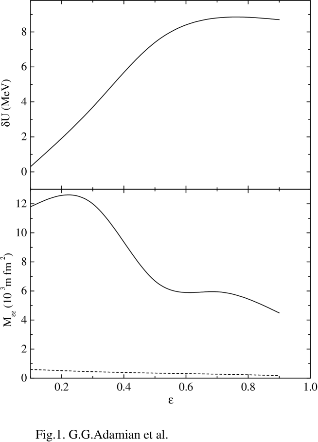
FIG. 1.: Dependence of the mass parameter $M_{\varepsilon\varepsilon}$ (lower part) and of the shell correction $\delta U$ (upper part) on $\varepsilon$ for the system ¹¹⁰Pd+¹¹⁰Pd at $\lambda=1.6$. In the calculation of $M_{\varepsilon\varepsilon}$ an excitation energy of 30 MeV of the DNS and adiabatic single particle states are used. The mass parameter $M_{\varepsilon\varepsilon}^{WW}$ calculated in the Werner-Wheeler approximation is presented by a dashed line in the lower part. Units: $m$ fm² with $m=$nucleon mass.

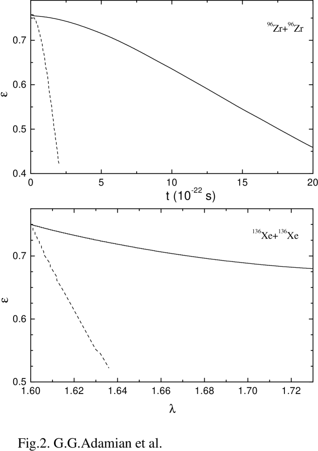
FIG. 2.: Upper part: Time-dependence of the neck parameter $\varepsilon$ in the system ⁹⁶Zr+⁹⁶Zr calculated with microscopical (solid curve) and Werner–Wheeler (dashed curve) mass parameters. Lower part: Trajectories in the ($\lambda$,$\varepsilon$)-plane calculated for the system ¹³⁶Xe+¹³⁶Xe with microscopical mass parameters (solid curve) and with Werner–Wheeler mass parameters (dashed curve). The end points of the solid and dashed curves in the drawing are at time $t=2\times 10^{-21}$s and $t=2\times 10^{-22}$s, respectively.

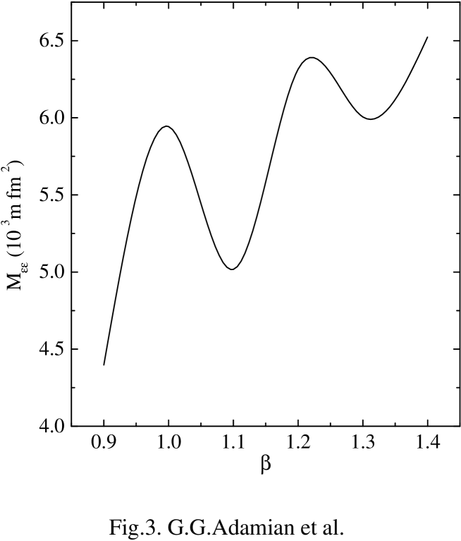
FIG. 3.: Mass parameter $M_{\varepsilon\varepsilon}$ as a function of deformation $\beta$ calculated for the system ¹¹⁰Pb+¹¹⁰Pb at the touching configuration with excitation energy 30 MeV and adiabatic single particle states. Units: $m$ fm² with $m=$nucleon mass.

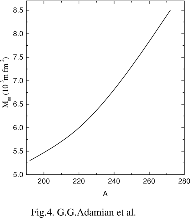
FIG. 4.: Mass parameter $M_{\varepsilon\varepsilon}$ as a function of the mass number $A$ of symmetric systems ($\eta=0$) calculated with adiabatic single particle states for $\beta_{i}=1$, $\lambda=1.6$, and $\varepsilon=0.75$. Units: $m$ fm² with $m=$nucleon mass.

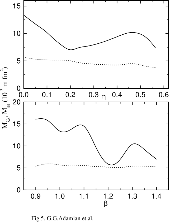
FIG. 5.: Upper part: Mass parameters $M_{\lambda\lambda}$ (solid line) and $M_{\varepsilon\varepsilon}$ (dotted line) as functions of mass asymmetry $\eta$ at the touching configuration for DNS which leads to the same compound nucleus ²²⁰U. The value of the neck coordinate is $\varepsilon$=0.75 and excitation energy of the DNS is 30 MeV. The calculation is done with spherical nuclei. Lower part: The same as in the upper part, but as a function of deformation $\beta$ for the reaction ¹¹⁰Pd+¹¹⁰Pd ($\eta=0$). Diabatic single particle states are used. Units: $m$ fm² with $m=$nucleon mass.

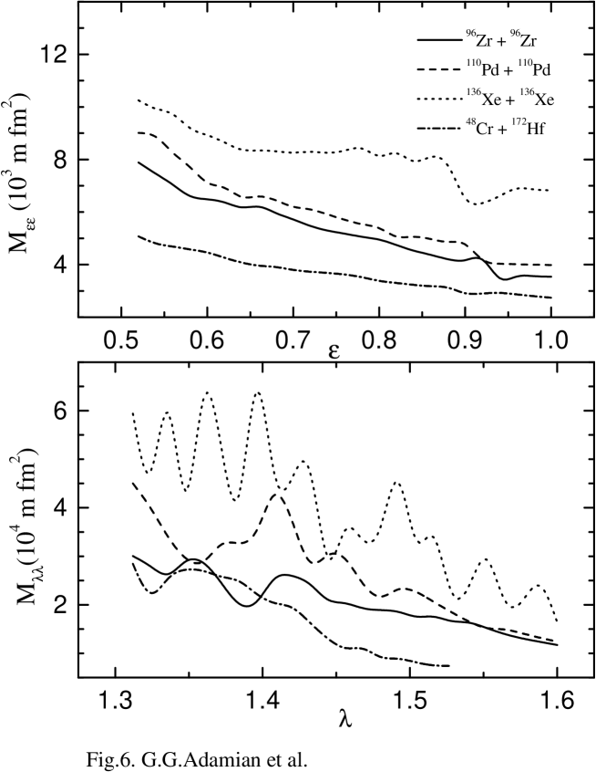
FIG. 6.: Upper part: Mass parameter $M_{\varepsilon\varepsilon}$ as a function of the neck coordinate $\varepsilon$ at the touching configuration in the reactions: ⁹⁶Zr+⁹⁶Zr (solid line), ¹¹⁰Pd+¹¹⁰Pd (dashed line), ¹³⁶Xe+¹³⁶Xe (dotted line) and ⁴⁸Ca+¹⁷²Hf (dashed–dotted line). The excitation energy of the DNS in these reactions is 30 MeV. Lower part: The same as in the upper part, but for $M_{\lambda\lambda}$ as a function of the elongation $\lambda$. Diabatic single particle states are used. Units: $m$ fm² with $m=$nucleon mass.

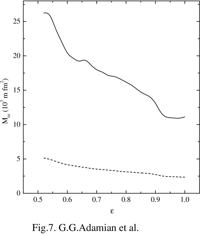
FIG. 7.: Mass parameter $M_{\varepsilon\varepsilon}$ as a function of $\varepsilon$ at the touching configuration in the ¹¹⁰Pd+¹¹⁰Pd reaction for temperatures $T_{0}=1$ MeV (solid line) and $1.5$ MeV (dashed line). Diabatic single particle states are used. Units: $m$ fm² with $m=$nucleon mass.

- [1] M. Brack, J. Damgaard, A.S. Jensen, H.C. Pauli, V.M. Strutinsky and C.Y. Wong, Rev. Mod. Phys. 44 (1972) 320.
- [2] G.D. Adeev, I.A. Gamalya and P.A. Cherdantsev, Soviet J. Nucl. Phys. 12 (1971) 148; Bulletin Academy of Science of USSR, Physics 36 (1972) 583.
- [3] J. Maruhn and W. Greiner, Z. Phys. A 251 (1972) 431.
- [4] J. Maruhn, W. Scheid and W. Greiner, in Heavy ion collisions. Ed. R. Bock (North-Holland, Amsterdam, 1980) vol. 2., p. 397.
- [5] W.J. Swiatecki, Progr. Part. Nucl. Phys. 4 (1980) 383; Phys. Scr. 24 (1981) 113.
- [6] V.V. Volkov, Deep inelastic nuclear reactions (Energoizdat, Moscow, 1982).
- [7] V.V. Volkov, in Proc. Int. School-Seminar on Heavy Ion Physics, Dubna, 1986 (JINR, Dubna, 1987) p.528; Izv. AN SSSR ser. fiz. 50 (1986) 1879; in Proc. Int. Conf. on Nuclear Reaction Mechanisms, Varenna, 1991, ed. E.Gadioli (Ricerca Scientifica, 1991) p.39.
- [8] P. Fröbrich, Phys. Rep. 116 (1984) 337.
- [9] W.U. Schröder and J.R. Huizenga, in Treatise on heavy-ion science. Ed. D.A. Bromley (Plenum, New York, 1984) vol. 2., p. 115.
- [10] N.V. Antonenko, E.A. Cherepanov, A.K. Nasirov, V.B. Permjakov and V.V. Volkov, Phys. Lett. B 319 (1993) 425; Phys. Rev. C 51 (1995) 2635; G.G. Adamian, N.V. Antonenko, W. Scheid, Nucl. Phys. A 618 (1997) 176; G.G. Adamian, N.V. Antonenko, W. Scheid, V.V. Volkov, Nucl. Phys. A 627 (1997) 332; A 633 (1998) 154. R.V. Jolos, A.K. Nasirov, A.I. Muminov, Europ.Phys.J. A 4 (1999) 246; E.A. Cherepanov, Pramana 23 (1999) 1.
- [11] G.G. Adamian, N.V. Antonenko, S.P. Ivanova and W. Scheid, Nucl. Phys. A 646 (1999) 29.
- [12] G.G. Adamian, N.V. Antonenko and Yu.M. Tchulvil’sky, Phys. Lett. B 451 (1999) 289.
- [13] A. Díaz-Torres, G.G. Adamian, N.V. Antonenko and W. Scheid, submitted for publication.
- [14] Yu.F. Smirnov and Yu.M. Tchulvil’sky, Phys. Lett. B 134 (1984) 25; O.F. Nemetz, V.G. Neudatchin, A.T. Rudchik, Yu.F. Smirnov and Yu.M. Tchuvil’sky, Nucleonic clusters in nuclei and the many-nucleon transfer reactions (Kiev: Naukova Dumka, 1988).
- [15] G. Bertsch, in Frontiers and borderlines in many–particles physics, Enrico Fermi School (CIV, Corso, 1988) p.41.
- [16] G.G.Adamian, N.V.Antonenko and R.V.Jolos, Nucl. Phys. A 584 (1995) 205.
- [17] J. Richert, T. Sami and H.A. Weidenmüller, Phys. Rev. C 26 (1982) 1018.
- [18] H. Hofmann, Phys. Rep. 284 (1997) 139.
- [19] F.A. Ivanyuk et al., Phys. Rev. C 55 (1997) 1730.
- [20] V. Schneider, J.Maruhn and W.Greiner, Z. Phys. A 323 (1986) 111.
- [21] W. Nörenberg, Phys. Lett. B 115 (1982) 179.
- [22] A. Lukasiak, W. Cassing and W. Nörenberg, Nucl. Phys. A 426 (1884) 181; W. Cassing and W. Nörenberg, Nucl. Phys. A 433 (1985) 467.
- [23] J.R. Primack, Phys. Rev. Lett. 17 (1966) 539.
- [24] J.J. Griffin, Nucl. Phys. A 170 (1971) 395.
- [25] T. Lederberger and H.C. Pauli, Nucl. Phys. A 207 (1973) 1.
- [26] V.M. Kolomietz and P.J. Siemens, Nucl. Phys. A 314 (1979) 141.
- [27] S. Yamaji, F.A. Ivanyuk and H. Hofmann, Nucl.Phys. A 612 (1997) 1.
- [28] W. Greiner and J.A. Maruhn, Nuclear Models (Springer-Verlag, Berlin/Heidelberg, 1996).
- [29] F.A. Ivanyuk, Z. Phys. A 334 (1989) 69; F.A. Ivanyuk and K.R.Pomorski, Phys. Rev. C 53 (1996) 1861.
- [30] H. Hofmann et al, Nucl. Phys. A 598 (1996) 187.
- [31] X. Wu et al., Phys. Rev. Lett. 79 (1997) 4542.
- [32] K. Fujikawa and H. Terashima, Phys. Rev. E 58 (1998) 7063.
- [33] J. Schirmer, S. Knaak and G. Güssmann, Nucl. Phys. A 199 (1973) 31.
- [34] A.Bohr and B.R.Mottelson, Nuclear Structure, vol. 1 (W.A. Benjamin, INC., Massachusetts, 1975).
- [35] A.S.Jensen, P.J.Siemens and H.Hofmann, in Nucleon-nucleon interaction and the many-body problem, Eds.: S.S.Wu and T.T.S.Kuo, World Scientific (1984).
- [36] A. Díaz-Torres, N.V. Antonenko and W. Scheid, Nucl. Phys. A 652 (1999) 61.
- [37] A.V. Ramayya et al., Phys. Rev. Lett. 81 (1998) 947.