NNLO Corrections to Nucleon-Nucleon Scattering
and Perturbative Pions

Abstract

The ${}^{1}S_{0}$, ${}^{3}S_{1}$, and ${}^{3}D_{1}$ nucleon-nucleon scattering phase shifts are calculated at next-to-next-to-leading order (NNLO) in an effective field theory. Predictions for the ${}^{1}P_{1}$, ${}^{3}P_{0,1,2}$, ${}^{1}D_{2}$, and ${}^{3}D_{2,3}$ phase shifts at this order are also compared with data. The calculations treat pions perturbatively and include the NNLO contributions from order $Q_{r}^{3}$ and $Q_{r}^{4}$ radiation pion graphs. In the ${}^{3}S_{1}$, ${}^{3}D_{1}$, and ${}^{3}P_{0,2}$ channels we find large disagreement with the Nijmegen partial wave analysis at NNLO. These spin triplet channels have large corrections from graphs with two potential pion exchange which do not vanish in the chiral limit. We compare our results to calculations within the Weinberg approach, and find that in some spin triplet channels the summation of potential pion diagrams seems to be necessary to reproduce the observed phase shifts. In the spin singlet channels the nonperturbative treatment of potential pions does not afford a significant improvement over the perturbative approach.

I Introduction

Understanding how nuclear forces emerge from the fundamental theory of Quantum Chromodynamics (QCD) remains an outstanding problem in theoretical physics. To study the physics of hadrons at scales where QCD is strongly coupled, it is useful to employ the technique of effective field theories. Model independent predictions for low energy nuclear phenomena can be made by using an effective Lagrangian which includes nucleons and pions as explicit degrees of freedom and all possible interactions that are consistent with the symmetries of the underlying QCD theory. This method, known as chiral perturbation theory, has been successfully applied to processes involving 0 and 1 nucleons (see e.g. [1, 2, 3]).

Weinberg [4] originally proposed using effective field theory for few body problems in nuclear physics. Weinberg’s procedure applies ordinary chiral perturbation theory power counting to the nucleon-nucleon potential and then solves the Schrödinger equation using this potential. Phenomenological studies of NN scattering phase shifts and deuteron properties which use this technique can be found in Refs. [5, 6, 7].

Application of effective field theory to two nucleon systems is complicated by the existence of a shallow bound state in the spin triplet channel and the large scattering length in the spin singlet channel. In Refs. [8, 9], Kaplan, Savage, and Wise (KSW) proposed a new power counting which accounts for these effects. This approach is more like ordinary chiral perturbation theory in that power counting is applied to the amplitude rather than the potential. All observables are expanded in powers of $Q/\Lambda$, where $Q$ is either $m_{\pi}$ or $p$ (the nucleon momentum), and $\Lambda$ is the range of the effective field theory. Because the S-wave scattering lengths (denoted by $a$) are large, powers of $pa$ must be summed to all orders [10]. This requires a nonperturbative treatment of the leading 4 nucleon operators with no derivatives. Higher derivative operators and pions are treated perturbatively. The perturbative treatment of pions makes it possible to obtain analytic expressions for amplitudes. One theoretically appealing aspect of the KSW power counting is that all ultraviolet divergences appearing in loop graphs are cancelled by contact operators appearing at either the same or a lower order in the expansion. This is in contrast with Weinberg’s approach in which unsubtracted divergences introduce cutoff dependence which is cancelled at higher orders in the expansion. The residual dependence on the cutoff gives an estimate of the size of higher order corrections.

It is clear from naive dimensional analysis that the KSW expansion will converge slowly. To see this, compare the contribution to the amplitude from single pion exchange and the pion box diagram:

$$\begin{picture}(25.0,20.0)(1.0,1.0)\put(-10.0,-6.0){\line(1,0){20.0}} \put(-10.0,14.0){\line(1,0){20.0}} \put(0.0,-5.0){\line(0,1){4.0}}\put(0.0,2.0){\line(0,1){4.0}}\put(0.0,9.0){\line(0,1){4.0}} \end{picture}\!\!\!\!\!\!={g_{A}^{2}\over 2f^{2}}\ A\!\left({p\over m_{\pi}}\right),\qquad\qquad\begin{picture}(25.0,20.0)(1.0,1.0)\put(-15.0,-6.0){\line(1,0){30.0}} \put(-15.0,14.0){\line(1,0){30.0}} \put(-8.0,-6.0){\line(0,1){4.0}}\put(-8.0,1.0){\line(0,1){4.0}}\put(-8.0,8.0){\line(0,1){4.0}} \put(8.0,-6.0){\line(0,1){4.0}}\put(8.0,1.0){\line(0,1){4.0}}\put(8.0,8.0){\line(0,1){4.0}} \end{picture}\!\!\!=\left({g_{A}^{2}\over 2f^{2}}\right)^{2}{Mm_{\pi}\over 4\pi}\ B\!\left({p\over m_{\pi}}\right)\,,$$ (1)

where $A,B$ are dimensionless functions. The factor of $M$, the nucleon mass, comes from performing the energy integral by contour integration and taking a pole from one of the nucleon propagators. The factor of $1/(4\pi)$ is an estimate of the size of the loop correction. (If a pion pole is taken the contribution is smaller by $m_{\pi}/M$ [11].) From Eq. (1) one expects an expansion parameter of order $(g_{A}^{2}m_{\pi}M)/(8\pi f^{2})\equiv m_{\pi}/\Lambda_{NN}\simeq 0.5$ [9]. This suggests that perturbative pions will converge, albeit slowly.

Many processes involving two nucleons have been computed to next-to-leading order (NLO) in the KSW expansion [12, 13]. The results of some of these calculations are reviewed in [14]. Typically, one finds 30%–40% errors at leading order (LO) and 10% errors at NLO. These results suggest an expansion parameter $Q/\Lambda\sim 1/3$ or $\Lambda\approx 400\,{\rm MeV}$. This is consistent with the estimate of the expansion parameter given above. Obviously, it is important to extend existing calculations to higher orders to see if the convergence of the expansion persists.

At the present time, few NNLO calculations are available in the theory with pions. The deuteron quadrupole moment is calculated to NNLO in Ref. [15]. The result of the NNLO calculation of the ${}^{1}S_{0}$ phase shift has been presented in Ref.[16, 17] and independently in Ref.[18]. However, these ${}^{1}S_{0}$ calculations are incomplete because the full order $Q$ contributions from radiation pion graphs were not included. The ${}^{3}S_{1}-{}^{3}D_{1}$ mixing parameter is calculated to NNLO in Ref.[19], where it is demonstrated that the expansion is converging for $p\leq 140\,{\rm MeV}$. For these momenta, the error is comparable to that of calculations within the Weinberg approach [6].

In this paper, we present NNLO calculations of the ${}^{1}S_{0}$, ${}^{3}S_{1}$, and ${}^{3}D_{1}$ phase shifts in nucleon-nucleon scattering, including contributions from radiation pions. At this order we find that the radiation pion diagrams have trivial momentum dependence and their effect cannot be distinguished from the contributions of a local operator. In the ${}^{1}S_{0}$ channel, the NNLO fit agrees with data to $<1$% accuracy for $p\simeq m_{\pi}$. In this channel, the KSW expansion works as expected. However, in the spin triplet channel we find that the expansion breaks down at NNLO. For the ${}^{3}S_{1}$ and ${}^{3}D_{1}$ phase shifts, the NNLO calculation actually does worse at fitting the data than the NLO prediction. In the ${}^{3}S_{1}$ channel, the NNLO corrections are as large as the NLO corrections for $p=m_{\pi}$. In the ${}^{3}D_{1}$ channel there is no sign of convergence for any value of $p$. We find that the failure of the EFT expansion in these two triplet channels is due to large non-analytic corrections that grow with $p$ coming from graphs with two potential pions. These terms do not appear in the spin singlet channel. The reason for the difference in the quality of the perturbative expansions in the two channels is that the potential between nucleons arising from pion exchange is much more singular in the spin triplet channel than in the singlet channel. We elaborate on this point in section V of the paper.

Next, we examine the NNLO predictions for the $P$ and $D$ wave phase shifts drawing on results from Ref. [11]. At LO these phase shifts vanish. In these channels the only contributions at NLO and NNLO come from potential pion exchange. Contact interaction and radiative pion contributions do not enter until higher order. Thus predictions for these phase shifts contain no free parameters, and it is possible to unambiguously test the perturbative treatment of pions. In the spin singlet channels (${}^{1}P_{1}$, ${}^{1}D_{2}$) corrections from two potential pion exchange are small, and the errors at $p=m_{\pi}$ are (13%, 33%). At $p=m_{\pi}$, the NNLO predictions for the ${}^{3}P_{1}$, ${}^{3}D_{2}$ channels have errors of the expected size (15%, 8%). In the ${}^{3}P_{0}$, ${}^{3}P_{2}$ channels errors are bigger than expected (170%, 52%). Like the ${}^{3}S_{1}$ and ${}^{3}D_{1}$ channels, these spin triplet channels have non-analytic contributions that grow with $p$.

Our final section includes a comparison of our calculations with those of Refs.[6, 7] which use the Weinberg approach. In spin singlet channels the corrections obtained by summing perturbative potential pion exchange to all orders are negligible. In particular, in the ${}^{1}P_{1}$ and ${}^{1}D_{2}$ channels, single pion exchange gives the same answer as the LO Weinberg calculation which treats potential pions nonperturbatively. Here corrections from soft and radiation pion graphs as well as contact interactions appear to be much more important. In the KSW expansion, these effects appear at one higher order than the results presented in this paper.

In some spin triplet channels (${}^{3}S_{1}$, ${}^{3}P_{1}$, ${}^{3}D_{1}$) the summation of potential pions gives significant improvement relative to the calculation which treats the pion perturbatively. There are also spin triplet channels where nonperturbative potential pions seem to be less important than soft pion graphs and four nucleon operators. This is true in the ${}^{3}P_{0}$ and ${}^{3}P_{2}$ channels, where the LO calculation in the Weinberg scheme does no better than the LO term in the KSW expansion. Finally, in the ${}^{3}D_{2,3}$ channels, the KSW expansion at NNLO gives predictions that are as accurate as the NNLO Weinberg calculations and so a nonperturbative treatment of pions does not seem to be necessary in these channels.

The rest of the paper will be organized as follows. In section II, the formalism relevant for our calculation is introduced. We define all operators appearing in the Lagrangian to the order we are working and discuss the solution to their renormalization group equations (RGE). Solving the RGE perturbatively ensures that observables are renormalization scale independent, as in pion chiral perturbation theory. We also discuss our method for fitting the constants at each order in the expansion. In section III, expressions are presented for the ${}^{1}S_{0}$, ${}^{3}S_{1}$ and ${}^{3}D_{1}$ amplitudes up to NNLO. Detailed comparison of the theoretical phase shifts with the Nijmegen phase shift analysis [20] appears in this section. In Section IV, we look at NLO and NNLO contributions to nucleon-nucleon scattering in the ${}^{1}P_{1}$, ${}^{3}P_{0,1,2}$, ${}^{1}D_{2}$, and ${}^{3}D_{2,3}$ waves. In the final section, we discuss our results and their implications for the perturbative treatment of pions. Details of the calculations are contained in the Appendices. In Appendix A we describe a trace formalism for projecting partial wave amplitudes from Feynman diagrams. In Appendix B we give explicit expressions for all individual graphs at NNLO, except for graphs involving radiation pions. We also describe a general strategy for analytically evaluating massive non-relativistic multi-loop Feynman diagrams. In Appendix C, the S-wave radiation pion contribution is discussed in detail. The power counting for radiation and soft pions is reviewed and the complete order $Q$ contribution is evaluated.

II Formalism

In this paper, we will follow the notation in Refs.[9, 19, 21]. The relevant Lagrangian for NN scattering at NNLO is

$${\cal L} = \frac{f^{2}}{8}{\rm Tr}\,(\partial^{\mu}\Sigma\>\partial_{\mu}\Sigma^{\dagger})+\frac{f^{2}\omega}{4}\,{\rm Tr}(m_{q}\Sigma+m_{q}\Sigma^{\dagger})+N^{\dagger}\bigg{(}iD_{0}+\frac{\vec{D}^{2}}{2M}\bigg{)}N$$ (2)

$$+ \frac{ig_{A}}{2}\,N^{\dagger}\sigma_{i}(\xi\partial_{i}\xi^{\dagger}-\xi^{\dagger}\partial_{i}\xi)N-{C_{0}^{(s)}}{\cal O}_{0}^{(s)}+\frac{C_{2}^{(s)}}{8}{\cal O}_{2}^{(s)}-{D_{2}^{(s)}}\omega{\rm Tr}(m^{\xi}){\cal O}_{0}^{(s)}$$ (3)

$$- \frac{{C_{4}^{(s)}}}{64}{\cal O}_{4}^{(s)}+\frac{E_{4}^{(s)}}{8}\omega{\rm Tr}(m^{\xi}){\cal O}_{2}^{(s)}-\frac{D_{4}^{(s)}}{2}\omega^{2}\Big{\{}{\rm Tr}^{2}(m^{\xi})+2{\rm Tr}[(m^{\xi})^{2}]\Big{\}}{\cal O}_{0}^{(s)}$$ (4)

$$- C_{2}^{(SD)}\,{\cal O}_{2}^{(SD)}+\ldots\,.$$ (5)

Here $g_{A}=1.25$ is the nucleon axial-vector coupling, $\Sigma=\xi^{2}=\exp(2\,i\,\Pi/f)$ where

$$\Pi=\left(\begin{array}[]{cc}\pi^{0}/\sqrt{2}&\pi^{+}\\ \pi^{-}&-\pi^{0}/\sqrt{2}\end{array}\right)\,,$$ (8)

$f=131\,{\rm MeV}$ is the pion decay constant, the chiral covariant derivative is $D_{\mu}=\partial_{\mu}+\frac{1}{2}(\xi\partial_{\mu}\xi^{\dagger}+\xi^{\dagger}\partial_{\mu}\xi)$, and $m^{\xi}=\frac{1}{2}(\xi m_{q}\xi+\xi^{\dagger}m_{q}\xi^{\dagger})$, where $m_{q}={\rm diag}(m_{u},m_{d})$ is the quark mass matrix. At the order we are working $\omega{\rm Tr}(m^{\xi})=\omega(m_{u}+m_{d})=m_{\pi}^{2}=(137\,{\rm MeV})^{2}$. In Eq. (2), $s={}^{1}S_{0}$ or ${}^{3}S_{1}$. Below this superscript will be dropped when it is clear from the context which channel is being referred to or when the reference is to both channels. The two-body nucleon operators are:

$${\cal O}_{0}^{(s)} = (N^{T}P^{(s)}_{i}N)^{\dagger}(N^{T}P^{(s)}_{i}N)\,,$$ (9)

$${\cal O}_{2}^{(s)} = (N^{T}P^{(s)}_{i}N)^{\dagger}(N^{T}P^{(s)}_{i}\>\tensor{\nabla}^{\,2}N)+h.c.\,,$$ (10)

$${\cal O}_{4}^{(s)} = (N^{T}P^{(s)}_{i}N)^{\dagger}(N^{T}P_{i}^{(s)}\>\tensor{\nabla}^{\,4}N)+h.c.+2(N^{T}P_{i}^{(s)}\tensor{\nabla}^{\,2}N)^{\dagger}(N^{T}P_{i}^{(s)}\>\tensor{\nabla}^{\,2}N)\,,$$ (11)

$${\cal O}_{2}^{(SD)} = (N^{T}P^{(^{3}S_{1})}_{i}N)^{\dagger}(N^{T}P^{(^{3}D_{1})}_{i}N)+h.c.\,,$$ (12)

where the projection matrices are

$$P_{i}^{({}^{1}\!S_{0})}={(i\sigma_{2})\,(i\tau_{2}\tau_{i})\over 2\sqrt{2}}\,,\qquad P_{i}^{({}^{3}\!S_{1})}={(i\sigma_{2}\sigma_{i})\,(i\tau_{2})\over 2\sqrt{2}}\,,$$ (13)

$$P_{i}^{({}^{3}\!D_{1})}=\frac{n}{4\sqrt{n-1}}\>\Big{(}\tensor{\nabla}_{i}\tensor{\nabla}_{j}-\frac{\delta_{ij}}{n}\>\tensor{\nabla}^{\,2}\Big{)}\>P_{j}^{({}^{3}\!S_{1})}\,,$$ (14)

and $\tensor{\nabla}=\overleftarrow{\nabla}-\overrightarrow{\nabla}$. The derivatives in Eqs. (9) and (13) should really be chirally covariant, however, only the ordinary derivatives are needed for the calculations in this paper.

Ultraviolet divergences are regulated using dimensional regularization. All spin and isospin traces are done in $n$ dimensions, where $d=n+1$ is the space-time dimension. Regulating the theory in this way preserves the chiral and rotational symmetry of the theory as well as the Wigner symmetry [22, 23] of the leading order Lagrangian, as discussed in Ref.[19].

The KSW power counting is manifest in renormalization schemes such as power divergence subtraction (PDS) [8, 9] or off-shell momentum subtraction (OS) [24, 25, 21]. (In this paper the PDS scheme will be used.) In these schemes the coefficients of the S-wave operators in Eq. (9) scale as $C_{2n}^{(s)}\sim 1/(M\Lambda^{n}\mu^{n+1})$, where $\mu$ is the renormalization scale, and $\Lambda$ is the range of the effective field theory. The renormalization scale is chosen to be on the order of the nucleon momentum $p$ which is of order $m_{\pi}$. Letting $\mu\sim p\sim m_{\pi}\sim Q$ the scaling of the coefficients in Eq. (2) is:

$${\rm LO} : \qquad C_{0}^{(s)}(\mu)\sim 1/Q$$ (15)

$${\rm NLO} : \qquad p^{2}\,C_{2}^{(s)}(\mu)\sim Q^{0},\,\,\,m_{\pi}^{2}\,D_{2}^{(s)}(\mu)\sim Q^{0}$$ (16)

$${\rm NNLO} : \qquad p^{4}\,C_{4}^{(s)}(\mu)\sim Q,\,\,\,m_{\pi}^{2}p^{2}\,E_{4}^{(s)}(\mu)\sim Q,\,\,\,m_{\pi}^{4}\,D_{4}^{(s)}(\mu)\sim Q\,,\,\,\,p^{2}C_{2}^{(SD)}(\mu)\sim Q\,.$$ (17)

Note that from simple dimensional analysis one would expect these coefficients to scale as $C_{2n}\sim 1/(M\Lambda^{2n+1})$. However, these coefficients are larger than naive dimensional analysis predicts because the theory flows to a non-trivial fixed point for $a\to\pm\infty$. (See Refs. [9, 26, 27] for a more detailed explanation.) Since $C_{0}^{(s)}(\mu)\sim 1/Q$, and each nucleon loop gives a factor of $Q$, power counting demands that graphs with $C_{0}$’s be summed to all orders. This sums all powers of $ap$. Operators with derivatives or insertions of the quark mass matrix scale as $Q^{n}$, $n\geq 0$, and are treated perturbatively.

In Eq. (2) we have not included four nucleon operators for partial waves with $L\geq 1$ because these operators enter at order $Q^{2}$ or higher. For example, the coefficients of the four P-wave operators with two derivatives are not enhanced by the renormalization group flow near the fixed point and therefore scale as $1/(M\Lambda^{3})$. Thus, these P-wave terms in the Lagrangian are order $Q^{2}/(M\Lambda^{3})$. As a result the order $Q$ predictions for partial waves with $L\geq 1$ come completely from pion exchange and have no free parameters.

There is another term in the Lagrangian in Eq. (2) with an S-wave four-derivative operator distinct from ${\cal O}_{4}^{(s)}$, ${\cal L}=\tilde{C}_{4}^{(s)}\>\tilde{\cal O}_{4}^{(s)}$ where

$$\tilde{\cal O}_{4}^{(s)} = \Big{[}(N^{T}P^{(s)}_{i}N)^{\dagger}(N^{T}P_{i}^{(s)}\>\tensor{\nabla}^{\,4}N)+h.c.-2(N^{T}P_{i}^{(s)}\tensor{\nabla}^{\,2}N)^{\dagger}(N^{T}P_{i}^{(s)}\>\tensor{\nabla}^{\,2}N)\Big{]}\,.$$ (18)

For the process $N(p_{1})N(p_{2})\to N(p_{3})N(p_{4})$ this operator vanishes on-shell since energy-momentum conservation gives $(\vec{p}_{1}-\vec{p}_{2})^{2}=(\vec{p}_{3}-\vec{p}_{4})^{2}$. In deriving the RGE’s only on-shell amplitudes are relevant. In fact the off-shell Green’s functions do not have to be $\mu$ independent, as illustrated by the off-shell $C_{2}$ amplitude given in Eq. (LABEL:offC2) of Appendix C. Thus, to derive an RGE for $\tilde{C}_{4}^{(s)}(\mu)$ it is necessary to consider an on-shell process in which this coefficient gives a non-zero contribution. Although $\tilde{C}_{4}^{(s)}(\mu)$ does not contribute to NN scattering, it may contribute to interactions with photons when the operator in Eq. (18) is gauged. Diagrams with two ${\cal O}_{2}^{(s)}$ operators renormalize ${\cal O}_{4}^{(s)}$ making $C_{4}^{(s)}(\mu)\sim 1/\mu^{3}$. The fact that ${\cal O}_{4}^{(s)}$ rather than ${\cal O}_{4}^{(s)}-\tilde{\cal O}_{4}^{(s)}$ has an enhanced coefficient differs from the conclusion in Ref. [28].

Relativistic corrections contribute at order $Q$ to the S-wave amplitudes. They are suppressed relative to the leading order amplitude by $(Q/M)^{2}$ rather than $(Q/\Lambda)^{2}$. In Ref.[28] these corrections are computed and found to be negligible relative to other order $Q$ contributions. Therefore they are left out of our analysis.

For momenta $p\gtrsim m_{\pi}$ pions should be included in the theory. There are three types of contributions from pions: radiation, potential, and soft. In evaluating non-relativistic loop diagrams the energy integrals are performed using contour integration. When the residue of a nucleon pole is taken the pion propagators in the loop are potential pions. When the residue of a pion pole is taken the pion will be either radiation or soft. Potential pion exchange scales as $Q^{0}$, and is therefore perturbative. Radiation and soft pions begin to contribute at order $Q$ and $Q^{2}$ respectively. The power counting for pions is discussed in detail in Appendix C. Because pion exchange is treated perturbatively the dominant scaling of the $C_{2n}(\mu)$ coefficients is the same as in the theory without pions.

The $Q$ scaling in Eq. (15) can be determined by computing the beta functions for the four nucleon couplings appearing in Eq. (2) to the order we are working. The procedure used for computing beta functions in the PDS scheme is described briefly in Appendix B and in detail in Ref. [21]. Our results are slightly different than Ref.[21] because all spin and isospin traces are performed in $n$ dimensions rather than 3 dimensions. For the ${}^{1}S_{0}$ channel, the beta functions to NNLO are:

$$\mu{\partial\over\partial\mu}C_{0} = {M\mu\over 4\pi}(C_{0})^{2}\left[1+2{g_{A}^{2}\over 2f^{2}}{M\mu\over 4\pi}+3\left({g_{A}^{2}\over 2f^{2}}{M\mu\over 4\pi}\right)^{2}\right]\,,$$ (19)

$$\mu{\partial\over\partial\mu}C_{2} = 2{M\mu\over 4\pi}C_{0}C_{2}\left(1+2{g_{A}^{2}\over 2f^{2}}{M\mu\over 4\pi}\right)\,,$$ (20)

$$\mu{\partial\over\partial\mu}D_{2} = 2{M\mu\over 4\pi}C_{0}D_{2}\left(1+2{g_{A}^{2}\over 2f^{2}}{M\mu\over 4\pi}\right)+{g_{A}^{2}\over 2f^{2}}\left({M\over 4\pi}\right)^{2}(C_{0})^{2}$$ (22)

$$+2\left({Mg_{A}^{2}\over 8\pi f^{2}}\right)^{2}C_{0}\left(1+{M\mu\over 4\pi}C_{0}\right)+\beta_{D_{2}}^{{\rm rad}}\,,$$

$$\mu{\partial\over\partial\mu}C_{4} = {M\mu\over 4\pi}\Big{[}2\,C_{0}C_{4}+(C_{2})^{2}\Big{]}\,,$$ (23)

$$\mu{\partial\over\partial\mu}E_{4} = {M\mu\over 4\pi}\Big{[}2\,C_{0}E_{4}+2D_{2}\,C_{2}\Big{]}+2\,C_{2}\,C_{0}\,{g_{A}^{2}\over 2f^{2}}\left({M\over 4\pi}\right)^{2}\,,$$ (24)

$$\mu{\partial\over\partial\mu}D_{4} = {M\mu\over 4\pi}\Big{[}2\,C_{0}D_{4}+(D_{2})^{2}\Big{]}+2\,D_{2}\,C_{0}\,{g_{A}^{2}\over 2f^{2}}\left({M\over 4\pi}\right)^{2}\,,$$ (25)

where the contribution $\beta_{D_{2}}^{{\rm rad}}$ from radiation pions is given in Eq. (C65). All coupling constants are functions of $\mu$. In the ${}^{3}S_{1}$ channel, the beta functions for $C_{0}$, $C_{2}$, and $D_{2}$ are:

$$\mu{\partial\over\partial\mu}C_{0} = {M\mu\over 4\pi}(C_{0})^{2}\left(1+2{g_{A}^{2}\over 2f^{2}}{M\mu\over 4\pi}\right)+4{M\mu\over 4\pi}\left({g_{A}^{2}\over 2f^{2}}\right)^{2}\,,$$ (26)

$$\mu{\partial\over\partial\mu}C_{2} = 2{M\mu\over 4\pi}C_{0}C_{2}\left(1+2{g_{A}^{2}\over 2f^{2}}{M\mu\over 4\pi}\right)+12\left({Mg_{A}^{2}\over 8\pi f^{2}}\right)^{2}C_{0}\left(1+{M\mu\over 4\pi}C_{0}\right)\,,$$ (27)

$$\mu{\partial\over\partial\mu}D_{2} = 2{M\mu\over 4\pi}C_{0}D_{2}\left(1+2{g_{A}^{2}\over 2f^{2}}{M\mu\over 4\pi}\right)+{g_{A}^{2}\over 2f^{2}}\left({M\over 4\pi}\right)^{2}(C_{0})^{2}$$ (29)

$$+7\left({Mg_{A}^{2}\over 8\pi f^{2}}\right)^{2}C_{0}\left(1+{M\mu\over 4\pi}C_{0}\right)+\beta_{D_{2}}^{{\rm rad}}\,,$$

and the beta functions for $C_{4}$, $E_{4}$ and $D_{4}$ are identical to those in the ${}^{1}S_{0}$ channel. (We have corrected a sign error in the $C_{2}^{(^{3}S_{1})}$ beta function computed in Ref. [29].) The running of $C_{2}^{SD}(\mu)$ is discussed in Ref. [19]. Terms in the beta functions that vanish as $\mu\to 0$ are from linear power divergences and are renormalization scheme dependent. These terms are necessary for a consistent power counting near the $a\to\pm\infty$ fixed points. Taking $g_{A}\to 0$ gives the dominant power contributions, and these terms are the same in renormalization schemes with a manifest power counting like PDS or OS. Finally, terms that do not vanish as $\mu\to 0$ correspond to logarithmic divergences and are scheme independent.

It is desirable that the amplitude, and hence all physical quantities, like the scattering length, be $\mu$ independent at each order in the expansion. This can be accomplished by expanding the coupling constants in $Q$ [25]:

$$C_{0} \rightarrow C_{0}+C_{0}^{(0)}+C_{0}^{(1)}$$ (30)

$$C_{2} \rightarrow C_{2}+C_{2}^{(-1)}$$ (31)

$$D_{2} \rightarrow D_{2}+D_{2}^{(-1)}\,.$$ (32)

The first piece of $C_{0}$ is treated nonperturbatively (i.e. $C_{0}\sim Q^{-1}$), while $C_{0}^{(0)}\sim Q^{0},C_{0}^{(1)}\sim Q$. Because of the perturbative expansion of the couplings in Eq. (30) there are ten constants of integration that appear in the calculation of the NNLO S-wave phase shifts. However, the NNLO amplitude depends only on six independent linear combinations of these constants. The coupling constants are also subject to two further constraints:

1. At this order, $C_{4}$, $E_{4}$ and $D_{4}$ are determined entirely in terms of lower order couplings as a consequence of solving the RGE’s and applying the KSW power counting.

2. Spurious double and triple poles in the NLO and NNLO amplitudes must be cancelled in order to obtain a good fit at low momentum.

An example of constraint 1 is provided by the solution of the RGE for $C_{4}$ given in Eq. (19) [9]:

$$C_{4}={(C_{2})^{2}\over C_{0}}+\rho{M\over 4\pi}(C_{0})^{2}\,,$$ (33)

where $\rho$ is a constant of integration. In the theory without pions, $\rho$ is proportional to the shape parameter, which is $\sim Q^{0}$ in the KSW power counting. In the theory with pions $\rho\sim Q^{0}$ too, since its size is determined by the scale $\Lambda$. Therefore, $(C_{2})^{2}/C_{0}\sim Q^{-3}$, while $\rho(C_{0})^{2}M/(4\pi)\sim Q^{-2}$. The second term is subleading in the $Q$ expansion, and should be omitted at NNLO, so $C_{4}=(C_{2})^{2}/C_{0}$. Solving Eq. (19) gives similar relations for $E_{4}$, and $D_{4}$:

$$E_{4}={2C_{2}D_{2}\over C_{0}}+{\cal O}(Q^{-2})\,,\qquad\quad D_{4}={(D_{2})^{2}\over C_{0}}+{\cal O}(Q^{-2})\,,$$ (34)

assuming that the constants of integration are order $Q^{0}$. The beta functions for $E_{4}$ and $D_{4}$ have contributions from chiral logarithms, which are determined by the $\ln(\mu)$ in $D_{2}$.

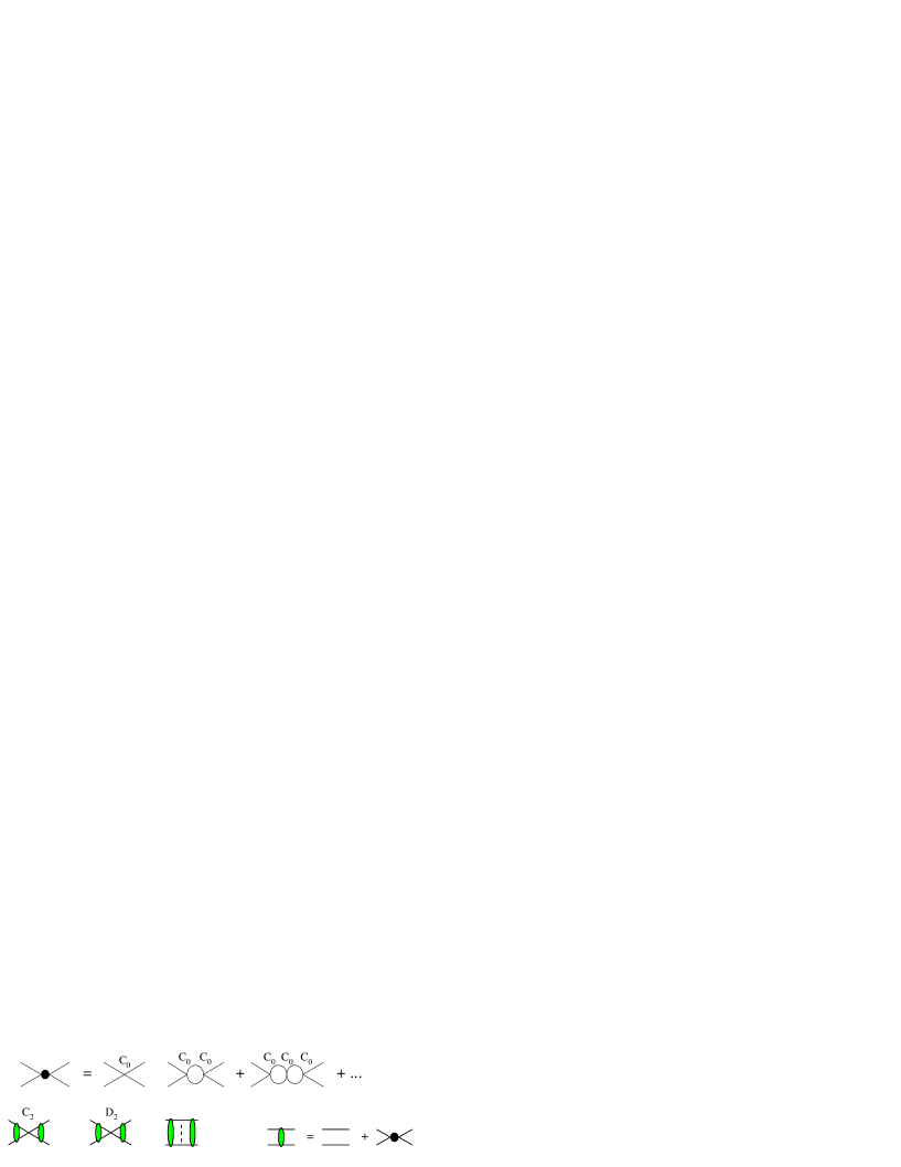
FIG. 1.: Order $1/Q$ (first row) and $Q^{0}$ (second row) diagrams for NN scattering. The solid lines are nucleons and the dashed line is a potential pion.

Constraint 2 is due to the nonperturbative treatment of $C_{0}$, which gives rise to spurious poles at higher orders in the expansion. The leading order amplitude ${\cal A}_{-1}$ has a simple pole at $p=i\gamma$. The NLO amplitude is proportional to ${\cal A}_{-1}^{2}$, and therefore has a double pole, while the NNLO amplitude has terms proportional to ${\cal A}_{-1}^{2}$ and ${\cal A}_{-1}^{3}$. To obtain a good fit at low momentum, parameters need to be fixed so that the amplitude has only a simple pole at each order in the expansion. This requires that ${\cal A}_{-1}$ have its pole in the correct location and that the residues of the spurious double and triple poles vanish. This requirement leads to the following good fit conditions [25]:

$$\left.{1\over{\cal A}_{-1}}\right|_{p=p^{*}}\!\!\!\!=0\,,\qquad\left.{{\cal A}_{0}\over({\cal A}_{-1})^{2}}\right|_{p=p^{*}}\!\!\!\!=0\,,\qquad\left.{{\cal A}_{1}\over{(\cal A}_{-1})^{2}}\right|_{p=p^{*}}\!\!\!\!=0\,,\qquad$$ (35)

where $p^{*}$ is the location of the pole. The second condition first appears at NLO, the third at NNLO. The residue of the triple pole in ${\cal A}_{1}$ vanishes by the second equation in Eq. (35). The first equation results in $\gamma=-ip^{*}$, while the other equations give constraints which eliminate two of the remaining parameters. In order to solve the constraints in Eq. (35) we must allow the coupling constants $C_{0}^{(0)}$ and $C_{0}^{(1)}$ to have non-analytic dependence on $m_{\pi}$. Ideally, all $m_{\pi}$ dependence should be explicit in the Lagrangian and the coupling $C_{0}$ should only depend on short distance scales. However, the fine tuning that results in the large scattering lengths is a consequence of a delicate cancellation between long and short distance contributions, and in order to put the pole in the physical location, one must induce explicit $m_{\pi}$ dependence in the perturbative parts of $C_{0}$ [16, 30]. Eq. (35) will be applied to both S-wave channels. After imposing these conditions, there is one free parameter at NLO and two free parameters at NNLO.

III Amplitudes and Phase Shifts

A ${}^{1}S_{0}$ channel

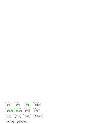
FIG. 2.: Order $Q$ contact interaction and potential pion graphs for the ${}^{1}S_{0}$ and ${}^{3}S_{1}$ channels. At this order the first three graphs do not introduce new parameters as explained in the text. Radiation pion diagrams with order $Q$ contributions are shown in Appendix C.

In this section, we present the NNLO calculation of the ${}^{1}S_{0}$ phase shift. At NLO the amplitude involves the diagrams in Fig. 1 calculated in Ref. [9]. Graphs contributing to the NNLO amplitude include those with one insertion of an order $Q$ operator and those with two insertions of either a potential pion or order $Q^{0}$ operator. These graphs are shown in Fig.2. A discussion of the techniques used to evaluate these graphs and explicit expressions for each individual graph are given in Appendix B. The NNLO amplitude also receives contributions from graphs with radiation pions which are discussed in Appendix C.

By expanding $\exp(2i\delta)=1+ipM{\cal A}/(2\pi)$ in powers of $Q$ we obtain expressions for the ${}^{1}S_{0}$ phase shift $\delta=\delta^{(0)}+\delta^{(1)}+\delta^{(2)}$ (where $\delta^{(n)}\sim Q^{n}$) in terms of the amplitudes ${\cal A}={\cal A}_{-1}+{\cal A}_{0}+{\cal A}_{1}$ (where $A_{n}\sim Q^{n}$),

$${\delta}^{(0)} = {1\over 2i}\,{\rm ln}\left(1+{ipM\over 2\pi}{\cal A}_{-1}\right)\,,\qquad{\delta}^{(1)}={pM\over 4\pi}{{\cal A}_{0}\over 1+{ipM\over 2\pi}{\cal A}_{-1}}\,,$$ (36)

$${\delta}_{0}^{(2)} = {pM\over 4\pi}{{\cal A}_{1}\over 1+{ipM\over 2\pi}{\cal A}_{-1}}-i\left({pM\over 4\pi}\right)^{2}\left({{\cal A}_{0}\over 1+{ipM\over 2\pi}{\cal A}_{-1}}\right)^{2}\,.$$ (37)

Our final result for the amplitude at NNLO is quite simple:

$${\cal A}_{-1} = -{4\pi\over M}{1\over\gamma+ip}\,,$$ (38)

$${{\cal A}_{0}} = -{\cal A}_{-1}^{2}(\zeta_{1}\,p^{2}+\zeta_{2}\,m_{\pi}^{2})$$ (40)

$$+{g_{A}^{2}\over 2f^{2}}{\cal A}_{-1}^{2}\Big{(}{Mm_{\pi}\over 4\pi}\Big{)}^{2}\bigg{[}{(\gamma^{2}-p^{2})\over 4p^{2}}{\rm ln}\Big{(}1+{4p^{2}\over m_{\pi}^{2}}\Big{)}-\,{\gamma\over p}{\rm tan}^{-1}\left({2p\over m_{\pi}}\right)\bigg{]}\,,$$

$${{\cal A}_{1}} = {{\cal A}_{0}^{2}\over{\cal A}_{-1}}-{\cal A}_{-1}^{2}\Big{(}\zeta_{3}\,m_{\pi}^{2}+\zeta_{4}\,p^{2}+\zeta_{5}{p^{4}\over m_{\pi}^{2}}\Big{)}+{{\cal A}_{0}}{Mg_{A}^{2}\over 8\pi f^{2}}\,{m_{\pi}^{2}\over p}\bigg{[}{\gamma\over 2p}\>{\rm ln}\Big{(}1+{4p^{2}\over m_{\pi}^{2}}\Big{)}$$ (44)

$$-{\rm tan}^{-1}\Big{(}{2p\over m_{\pi}}\Big{)}\bigg{]}+{M{\cal A}_{-1}^{2}\over 4\pi}\Big{(}{Mg_{A}^{2}\over 8\pi f^{2}}\Big{)}^{2}{m_{\pi}^{4}\over 4p^{3}}\Bigg{\{}2(\gamma^{2}-p^{2})\,{\rm Im}\,{\rm Li_{2}}\Big{(}{-m_{\pi}\over m_{\pi}-2ip}\Big{)}$$

$$-4\gamma\,p\>{\rm Re}\,{\rm Li_{2}}\Big{(}{-m_{\pi}\over m_{\pi}-2ip}\Big{)}-{\gamma\,p\,\pi^{2}\over 3}-(\gamma^{2}+p^{2})\bigg{[}{\rm Im}\,{\rm Li_{2}}\Big{(}{m_{\pi}+2ip\over-m_{\pi}+2ip}\Big{)}$$

$$+{\gamma\over 4p}\ln^{2}\Big{(}1+\frac{4p^{2}}{m_{\pi}^{2}}\Big{)}-\tan^{-1}\Big{(}\frac{2p}{m_{\pi}}\Big{)}\ln\Big{(}1+\frac{4p^{2}}{m_{\pi}^{2}}\Big{)}\bigg{]}\Bigg{\}}\,.$$

Using Eq. (38) it is easy to verify that the S-matrix is unitary to the order we are working. The six linearly independent constants appearing in the amplitude are $\gamma,\zeta_{1},\zeta_{2},\zeta_{3},\zeta_{4},\zeta_{5}$:

$$\gamma = \,\,{4\pi\over MC_{0}}+\mu\ \,,\qquad\quad\zeta_{1}=\,\left[{C_{2}\over(C_{0})^{2}}\right]\,,$$ (45)

$$\zeta_{2} = \left[{D_{2}\over(C_{0})^{2}}-{g_{A}^{2}\over 4f^{2}}\Big{(}{M\over 4\pi}\Big{)}^{2}{\rm ln}\Big{(}{\mu^{2}\over m_{\pi}^{2}}\Big{)}\right]+\frac{1}{m_{\pi}^{2}}\left[{C_{0}^{(0)}\over(C_{0})^{2}}+{g_{A}^{2}\over 2f^{2}}\Big{(}{M\over 4\pi}\Big{)}^{2}(\gamma^{2}\!-\!\mu^{2})\right]\,,$$ (46)

$$\zeta_{3} = -{g_{A}^{2}\over 2f^{2}}{Mm_{\pi}\over 4\pi}\left[{C_{2}\over(C_{0})^{2}}\right]+{1\over m_{\pi}^{2}}\left[{C_{0}^{(1)}\over(C_{0})^{2}}-{(C_{0}^{(0)})^{2}\over(C_{0})^{3}}-\left({g_{A}^{2}\over 2f^{2}}\right)^{2}\left({M\over 4\pi}\right)^{3}(\mu^{3}-\gamma^{3})\right]$$ (49)

$$-{2\gamma\over m_{\pi}^{2}}\,{Mg_{A}^{2}\over 8\pi f^{2}}\left[{C_{0}^{(0)}\over(C_{0})^{2}}+{g_{A}^{2}\over 2f^{2}}\left({M\over 4\pi}\right)^{2}(-\mu^{2}+\gamma^{2})\right]-2{M\gamma\over 4\pi}\Big{(}\frac{Mg_{A}^{2}}{8\pi f^{2}}\Big{)}^{2}\Big{(}\ln 2-\frac{3}{2}\Big{)}$$

$$+m_{\pi}^{2}\left\{{D_{4}\over(C_{0})^{2}}\!\!-\!{D_{2}^{2}\over(C_{0})^{3}}\right\}\!\!+\!\left[{D_{2}^{(-1)}\over(C_{0})^{2}}-{2D_{2}C_{0}^{(0)}\over(C_{0})^{3}}-{g_{A}^{2}\over f^{2}}{M\gamma\over 4\pi}{D_{2}\over(C_{0})^{2}}\right]+\zeta_{3}^{rad}\,,$$

$$\zeta_{4} = \left[{C_{2}^{(-1)}\over(C_{0})^{2}}-{2\,C_{2}\,C_{0}^{(0)}\over(C_{0})^{3}}-{g_{A}^{2}\over f^{2}}{M\gamma\over 4\pi}{C_{2}\over(C_{0})^{2}}\right]+m_{\pi}^{2}\ \left\{{E_{4}\over(C_{0})^{2}}-{2\,C_{2}\,D_{2}\over(C_{0})^{3}}\right\}\,,$$ (50)

$$\zeta_{5} = m_{\pi}^{2}\ \left\{{C_{4}\over(C_{0})^{2}}-{(C_{2})^{2}\over(C_{0})^{3}}\right\}\,.$$ (51)

$\zeta_{1}-\zeta_{5}$ are dimensionless constants. Note that $\zeta_{2}-\zeta_{5}$ include factors of $m_{\pi}$ and are not simply short distance quantities. After solving the RGE’s in Eq. (19) one finds that all quantities in square and curly brackets are separately $\mu$ independent. Furthermore, the quantities in curly brackets vanish at NNLO in the $Q$ expansion due to Eqs. (33) and (34). In Eq. (45) the order $Q$ radiation pion contributions appear in $\zeta_{3}^{rad}$ given in Eq. (C63) of Appendix C. At order $Q$, the effect of radiation pions turns out to be indistinguishable from corrections coming from contact interactions.

For the ${}^{1}S_{0}$ channel, the location of the pole is determined by solving

$$-{1\over a}+{r_{0}\over 2}(p^{*})^{2}-ip^{*}=0\,.$$ (52)

This fixes $\gamma=-7.88\,{\rm MeV}$. Note that adding the shape parameter correction to Eq. (52) changes the location of the pole by less than $0.01\%$. The NLO good fit condition in Eq. (35) relates the constants $\zeta_{1}$ and $\zeta_{2}$,

$$\zeta_{2}={\gamma^{2}\over m_{\pi}^{2}}\,\zeta_{1}-{M\over 4\pi}\,{g_{A}^{2}M\over 8\pi f^{2}}\,{\rm log}\left(1+{2\gamma\over m_{\pi}}\right)\,,$$ (53)

leaving one new parameter in the fit at NLO. At NNLO, $\zeta_{5}=0$ once we impose $C_{4}=C_{2}^{2}/C_{0}$. This leaves $\zeta_{3}$ and $\zeta_{4}$, which are related by the NNLO good fit condition

$$\zeta_{3}=\frac{\gamma^{2}}{m_{\pi}^{2}}\,\zeta_{4}+\Big{(}{Mg_{A}^{2}\over 8\pi f^{2}}\Big{)}^{2}{M\over 4\pi}\ {m_{\pi}^{2}\over\gamma}\bigg{[}{\rm Re}\,{\rm Li}\Big{(}{-m_{\pi}\over m_{\pi}+2\gamma}\Big{)}+\frac{\pi^{2}}{12}\bigg{]}\,.$$ (54)

Since $\zeta_{1}$ and $\zeta_{4}$ are multiplied by $\gamma^{2}/m_{\pi}^{2}$ in Eqs. (53) and (54) these conditions basically fix the values of $\zeta_{2}$ and $\zeta_{3}$. We have chosen to fix $\zeta_{1}$ and $\zeta_{4}$ by performing a weighted least squares fit to the Nijmegen partial wave analysis[20]. The ranges $p=7-80\,{\rm MeV}$ and $p=7-200\,{\rm MeV}$ were used at NLO and NNLO respectively, with low momentum weighted more heavily. Using $M=939\,{\rm MeV}$, $m_{\pi}=137\,{\rm MeV}$, $g_{A}=1.25$, and $f=131\,{\rm MeV}$ the parameters for the ${}^{1}S_{0}$ channel are:

$${\rm NLO}: \qquad\zeta_{1}=0.216;\qquad\zeta_{2}=0.0318;$$ (55)

$${\rm NNLO}: \qquad\zeta_{1}=0.0777;\qquad\zeta_{2}=0.0313;\qquad\zeta_{3}=0.1831;\qquad\zeta_{4}=0.245\,.$$ (56)

The value of these parameters depend on the range of momentum used in the fit, for instance using the range $p=7-150\,{\rm MeV}$ at NLO gives $\zeta_{1}=0.25$. From the power counting we expect $\zeta_{1}\sim M/(4\pi\Lambda)$ at NLO and $\zeta_{1}+\zeta_{4}\sim M/(4\pi\Lambda)$ at NNLO. For $\Lambda\simeq 300\,{\rm MeV}$, $M/(4\pi\Lambda)\simeq 0.25$ in reasonable agreement with the fits.

    

FIG. 3.: Fit to the ${}^{1}S_{0}$ phase shift $\delta$. The solid line is the Nijmegen fit [20] to the data. In a), the long dashed, short dashed, and dotted lines are the LO, NLO, and NNLO results respectively. In b) we show two other NNLO fits with a different choice of parameters as described in the text.

The ${}^{1}S_{0}$ phase shift is shown in Fig. 3a. The solid line is the result of the Nijmegen phase shift analysis [20]. The ${}^{1}S_{0}$ phase shift has an expansion in powers of $Q$, and we plot the LO, NLO and NNLO results. The LO phase shift at $p=m_{\pi}$ is off by $48\%$. At NLO, the error is $17\%$. At NNLO, the error in the ${}^{1}S_{0}$ channel is less than $1\%$ at $p=m_{\pi}$, and the NNLO result gives improved agreement with the data even at $p\sim 400\,{\rm MeV}$.

Note that $\zeta_{3}\sim Q$ is larger than $\zeta_{2}\sim Q^{0}$ because from Eqs. (53) and (54), $\zeta_{3}/\zeta_{2}\sim m_{\pi}^{2}/(\gamma\Lambda_{NN})$. The parameter $\zeta_{2}$ is stable because it is fixed by the NLO good fit condition. On the other hand, $\zeta_{1}$ changes by a factor of 2.8 going from NLO to NNLO. One expects the value of coupling constants to change somewhat at each order in the expansion, but a factor of three difference is surprising. It is also disturbing that $\zeta_{4}$ is greater than $\zeta_{1}$, since, on the basis of the RGE and KSW power counting, it is expected that $\zeta_{4}<\zeta_{1}$ [21]. It is possible to do a fit and impose the constraints that $\zeta_{1}$ is close to its NLO value and $\zeta_{4}\leq\zeta_{1}$. If this is done the error at $p\simeq m_{\pi}$ is $\approx 10\%$, which is still an improvement relative to the NLO calculation and consistent with an expansion parameter of order $1/2$. This fit is shown as the dotted line in Fig. 3b.

The potential diagrams for the ${}^{1}S_{0}$ phase shift at NNLO were also computed by Rupak and Shoresh  [16]. To fit $\zeta_{1}$ and $\zeta_{4}$ they essentially demand that the experimental value of the effective range is reproduced at both NLO and NNLO. For the observable $\sin^{2}\delta$ at $p\simeq m_{\pi}$, they find $\simeq 80\%$, $\simeq 65\%$, and $\simeq 5\%$ errors at LO, NLO, and NNLO respectively [17].

Kaplan and Steele [30] have proposed that when the perturbative expansion of coupling constants is made the sub-dominant couplings should not be treated as new parameters. As an example, in their fitting procedure, $C_{2}^{(-1)}$ is given by

$$C_{2}^{(-1)}={2\,C_{2}\,C_{0}^{(0)}\over[C_{0}]^{2}}\,.$$ (57)

Imposing this condition fixes the value of $\zeta_{4}$ so that there is one less free parameter at NNLO. Kaplan and Steele motivated this fitting procedure by arguing that adding pions should only change long distance physics. Therefore, the number of free parameters in the theory with pions should be the same as in the pionless theory. It is worth pointing out that Ref. [30] made use of toy models in which the pions were represented as a contribution to the potential which is either a delta-shell removed a finite distance from the origin or a pure Yukawa. In these models it makes sense to think of the “pion” as purely long-distance because the pion effects are cleanly seperated even in the presence of loop corrections.

In a realistic effective field theory ultraviolet divergences from loops with pions do not allow a clean separation of long and short distance scales. As an example consider $C_{2}^{(^{3}S_{1})}=C_{2}+C_{2}^{(-1)}+C_{2}^{(0)}+\ldots$. Here $C_{2}$ first appears in the NLO diagrams in Fig. 1 and introduces a short distance effective range-like constant. At NNLO the diagram in Fig. 2k appears and has a logarithmic ultraviolet divergence that must be absorbed by $C_{2}^{(-1)}$. This induces a $\ln(\mu/K)$ dependence into the coupling $C_{2}^{(-1)}$ (as is clear from Eq. (81)). Since the constant $K$ is undetermined it is clear that $C_{2}^{(-1)}$ cannot be determined from lower order couplings. Note that if this $\ln(\mu)$ is instead absorbed into the leading order $C_{2}$ then this would induce additional $\ln(\mu)$ dependence into the part of the NNLO amplitude that depends on $C_{2}$.

In the ${}^{1}S_{0}$ channel $C_{2}^{(-1)}$ does not receive a logarithmic renormaliztion. However, there is a new logarithmic divergence that must be absorbed into $C_{2}^{(0)}$ coming from Fig. 8a [29]. Therefore, $C_{2}^{(0)}$ must be treated as a parameter. It is not possible to renormalize the theory in a $\mu$ independent way without introducing more parameters than exist in the pionless theory. The power law sensitivity to the choice of $\mu$ makes the $\mu$ independence of observables an essential criteria. Since, in general, higher order terms in the expansion of couplings receive ultraviolet renormalizations, we prefer to treat all $C_{2n}^{(m)}$ as free parameters whose size is only restricted by their RGE’s. This then implies that $\zeta_{4}$ is a free parameter in both the ${}^{1}S_{0}$ and ${}^{3}S_{1}$ channels. However, in the ${}^{1}S_{0}$ channel at NNLO imposing the relation in Eq. (57) does give a $\mu$ independent amplitude. In this case the result of the fit is shown by the dashed line in Fig. 3b. In general the choice of fit parameters is somewhat arbitrary, and a true test of the values can only be made by using them to predict an independent observable.

${}^{1}S_{0}$			$r_{0}$	$v_{2}$	$v_{3}$	$v_{4}$
	Fit[31]		$2.73\,{\rm fm}$	$-0.48\,{\rm fm^{3}}$	$3.8\,{\rm fm^{5}}$	$-17\,{\rm fm^{7}}$
	NLO		$2.65\,{\rm fm}$	$-3.3\,{\rm fm^{3}}$	$19\,{\rm fm^{5}}$	$-117\,{\rm fm^{7}}$
	NNLO		$2.63\,{\rm fm}$	$-1.2\,{\rm fm^{3}}$	$2.9\,{\rm fm^{5}}$	$-0.7\,{\rm fm^{7}}$

TABLE I.: Predictions for terms in the ${}^{1}S_{0}$ effective range expansion.

Finally, we present NNLO corrections to the higher order terms in the effective range expansion

$$p\,{\rm cot}(\delta)=-{1\over a}+{r_{0}\over 2}p^{2}+v_{2}p^{4}+v_{3}p^{4}+v_{4}p^{4}+\ldots\,.$$ (58)

Using the NLO expression for $p\,{\rm cot}(\delta)$, Cohen and Hansen [31] obtained predictions for $v_{2},v_{3}$ and $v_{4}$. At NLO, the effective field theory predictions for $v_{2}$, $v_{3}$, and $v_{4}$ disagree with the $v_{i}$ obtained from a fit to the Nijmegen phase shift analysis. The NNLO predictions for the shape parameters are shown in Table I. The prediction for $r_{0}$ is not better at NNLO than at NLO, but is still well within the expected errors. The NNLO $v_{i}$ predictions depend on $\zeta_{1}$ and $\zeta_{2}$. We see that the NNLO correction substantially reduces the discrepancy between the effective field theory prediction and the fit to the Nijmegen phase shift analysis, but the discrepancy is still quite large. This gives some evidence that the EFT expansion is converging on the true values of the $v_{i}$, albeit slowly. Effective field theory predictions for the shape parameters have been studied in toy models where one is able to go to very high orders in the $Q$ expansion [32]. In the toy models, the effective field theory did eventually reproduce the shape parameters, but the observed convergence is rather slow.

B ${}^{3}S_{1}$ channel

The S matrix for the ${}^{3}S_{1}$ and ${}^{3}D_{1}$ channels is $2\times 2$ and can be parameterized using the convention in Ref. [33] :

$$S={\mathbf{1}}+\frac{i\,Mp}{2\pi}\left(\begin{array}[]{cc}{\cal A}^{SS}&{\cal A}^{SD}\\ {\cal A}^{SD}&{\cal A}^{DD}\end{array}\right)=\left(\begin{array}[]{cc}e^{2i\bar{\delta}_{0}}\cos 2\bar{\epsilon}_{1}&i\,e^{i\bar{\delta}_{0}+i\bar{\delta}_{2}}\sin 2\bar{\epsilon}_{1}\\ i\,e^{i\bar{\delta}_{0}+i\bar{\delta}_{2}}\sin 2\bar{\epsilon}_{1}&e^{2i\bar{\delta}_{2}}\cos 2\bar{\epsilon}_{1}\end{array}\right)\,.$$ (63)

The phase shifts and mixing angle are expanded in powers of $Q/\Lambda$:

$$\bar{\delta}_{0}=\bar{\delta}_{0}^{(0)}+\bar{\delta}_{0}^{(1)}+\bar{\delta}_{0}^{(2)}+\ldots\,,\quad\bar{\delta}_{2}=0+\bar{\delta}_{2}^{(1)}+\bar{\delta}_{2}^{(2)}+\ldots\,,\quad\bar{\epsilon}_{1}=0+\bar{\epsilon}_{1}^{(1)}+\bar{\epsilon}_{1}^{(2)}+\ldots\,.$$ (64)

The phase shifts and mixing angles start at one higher order in $Q$ than the amplitudes because of the factor of $p$ in Eq. (63). In the PDS scheme, expressions for $\bar{\delta}_{0}^{(0,1)}$, $\bar{\delta}_{2}^{(1)}$, and $\bar{\epsilon}_{1}^{(1)}$ are given in Ref. [9]. The prediction for $\bar{\epsilon}_{1}^{(2)}$ is given in Ref. [19] and is discussed in section IIIC, and the prediction for $\bar{\delta}_{2}^{(2)}$ is given in section IIID.

Expressions for the terms in Eq. (64) in terms of the scattering amplitude are obtained by expanding both sides of Eq. (63) in powers of $Q$. This gives

$$\bar{\delta}_{0}^{(0)} = {1\over 2i}\,{\rm ln}\left(1+{ipM\over 2\pi}{\cal A}_{-1}^{SS}\right)\,,\qquad\bar{\delta}_{0}^{(1)}={pM\over 4\pi}{{\cal A}^{SS}_{0}\over 1+{ipM\over 2\pi}{\cal A}^{SS}_{-1}}\,,$$ (65)

$$\bar{\delta}_{0}^{(2)} = {pM\over 4\pi}{{\cal A}^{SS}_{1}\over 1+{ipM\over 2\pi}{\cal A}^{SS}_{-1}}-i\left({pM\over 4\pi}\right)^{2}\left[\left({{\cal A}^{SS}_{0}\over 1+{ipM\over 2\pi}{\cal A}^{SS}_{-1}}\right)^{2}+{({\cal A}^{SD}_{0})^{2}\over 1+{ipM\over 2\pi}{\cal A}^{SS}_{-1}}\right]\,.$$ (66)

In $\bar{\delta}^{(2)}_{0}$ the terms that depend on $A_{0}^{SS}$ and $A_{0}^{SD}$ are purely imaginary and cancel the imaginary part of the term proportional to ${\cal A}_{1}^{SS}$ as required by unitarity. The order $Q^{0}$ mixing amplitude is[9]

$${\cal A}_{0}^{SD} = \sqrt{2}\frac{Mg_{A}^{2}}{8\pi f^{2}}\>{\cal A}_{-1}^{SS}\bigg{\{}-\frac{3m_{\pi}^{3}}{4p^{2}}+\Big{(}\frac{m_{\pi}^{2}}{2p}+\frac{3m_{\pi}^{4}}{8p^{3}}\Big{)}\tan^{-1}\Big{(}\frac{2p}{m_{\pi}}\Big{)}+\frac{3\gamma m_{\pi}^{2}}{4p^{2}}-\frac{\gamma}{2}$$ (68)

$$\qquad\qquad\qquad\quad-\Big{(}\frac{\gamma m_{\pi}^{2}}{4p^{2}}+\frac{3\gamma m_{\pi}^{4}}{16p^{4}}\Big{)}\ln\Big{(}1+\frac{4p^{2}}{m_{\pi}^{2}}\Big{)}\bigg{\}}\,.$$

The diagrams which contribute to the ${}^{3}S_{1}$ amplitude up to NNLO are shown in Figs. 1 and 2 and give

$${\cal A}^{SS}_{-1} = -{4\pi\over M}{1\over\gamma+ip}\,,$$ (69)

$${{\cal A}^{SS}_{0}} = -\Big{[}{\cal A}^{SS}_{-1}\Big{]}^{2}(\zeta_{1}\,p^{2}+\zeta_{2}\,m_{\pi}^{2})$$ (71)

$$+\Big{[}{\cal A}^{SS}_{-1}\Big{]}^{2}{g_{A}^{2}\over 2f^{2}}\Big{(}{Mm_{\pi}\over 4\pi}\Big{)}^{2}\bigg{[}{(\gamma^{2}-p^{2})\over 4p^{2}}\>{\rm ln}\Big{(}1+{4p^{2}\over m_{\pi}^{2}}\Big{)}-\,{\gamma\over p}\>{\rm tan}^{-1}\left({2p\over m_{\pi}}\right)\bigg{]}\,,$$

$${{\cal A}_{1}^{SS}} = {[{\cal A}^{SS}_{0}]^{2}\over{\cal A}^{SS}_{-1}}+{ipM\over 4\pi}\Big{[}{\cal A}_{0}^{SD}\Big{]}^{2}+{{\cal A}^{SS}_{0}}\>{Mg_{A}^{2}\over 8\pi f^{2}}\>{m_{\pi}^{2}\over p}\bigg{[}{\gamma\over 2p}\>{\rm ln}\Big{(}1+{4p^{2}\over m_{\pi}^{2}}\Big{)}-{\rm tan}^{-1}\Big{(}{2p\over m_{\pi}}\Big{)}\bigg{]}$$ (72)

$$- \Big{[}{\cal A}^{SS}_{-1}\Big{]}^{2}\,\Big{(}\zeta_{3}\,m_{\pi}^{2}+\zeta_{4}\,p^{2}+\zeta_{5}{p^{4}\over m_{\pi}^{2}}\Big{)}$$ (73)

$$+ \Big{[}{\cal A}^{SS}_{-1}\Big{]}^{2}\,{M\over 4\pi}\,\Big{(}{Mg_{A}^{2}\over 8\pi f^{2}}\Big{)}^{2}\Bigg{[}{-6\gamma^{2}m_{\pi}^{3}+9\gamma m_{\pi}^{4}-3m_{\pi}^{5}\over 4p^{2}}+\ln 2\Big{(}\frac{9\gamma m_{\pi}^{6}}{4p^{4}}\!+\!\frac{3\gamma m_{\pi}^{4}}{2p^{2}}\!-\!\frac{9m_{\pi}^{7}}{4p^{4}}\!-\!\frac{3m_{\pi}^{5}}{p^{2}}\Big{)}$$ (80)

$$+\Big{(}6\,p^{2}\!+\!6m_{\pi}^{2}\!-\!\frac{3m_{\pi}^{4}}{4p^{2}}\!-\!\frac{9m_{\pi}^{6}}{8p^{4}}\Big{)}\bigg{[}{p^{2}\!-\!\gamma^{2}\over p}\tan^{-1}\Big{(}\frac{p}{m_{\pi}}\Big{)}-\gamma\,\ln\Big{(}1+\frac{p^{2}}{m_{\pi}^{2}}\Big{)}\bigg{]}$$

$$-\Big{(}\frac{3m_{\pi}^{5}}{p^{3}}\!+\!\frac{9m_{\pi}^{7}}{4p^{5}}\Big{)}\bigg{[}\gamma\,\tan^{-1}\Big{(}\frac{p}{m_{\pi}}\Big{)}-\frac{(\gamma^{2}-p^{2})}{4p}\ln\Big{(}1+\frac{p^{2}}{m_{\pi}^{2}}\Big{)}\bigg{]}$$

$$+\Big{(}\frac{9m_{\pi}^{7}}{8p^{5}}\!+\!\frac{3m_{\pi}^{5}}{2p^{3}}\!-\!\frac{9\gamma m_{\pi}^{6}}{8p^{5}}\!-\!\frac{3\gamma m_{\pi}^{4}}{4p^{3}}\!+\!\frac{\gamma m_{\pi}^{2}}{p}\Big{)}\bigg{[}\gamma\tan^{-1}\Big{(}\frac{2p}{m_{\pi}}\Big{)}+\frac{p}{2}\ln\Big{(}1+\frac{4p^{2}}{m_{\pi}^{2}}\Big{)}\bigg{]}$$

$$+\Big{(}\frac{9m_{\pi}^{8}}{32p^{7}}\!+\!\frac{3m_{\pi}^{6}}{4p^{5}}+\frac{3m_{\pi}^{4}}{4p^{3}}\Big{)}\Bigg{\{}2(\gamma^{2}\!-\!p^{2})\,{\rm Im}\,{\rm Li_{2}}\Big{(}{-m_{\pi}\over m_{\pi}\!-\!2ip}\Big{)}\!-\!4\gamma\,p\>{\rm Re}\,{\rm Li_{2}}\Big{(}{-m_{\pi}\over m_{\pi}\!-\!2ip}\Big{)}\!-\!{\gamma\,p\,\pi^{2}\over 3}$$

$$\ \ \ -(\gamma^{2}+p^{2})\bigg{[}{\rm Im}\,{\rm Li_{2}}\Big{(}{m_{\pi}\!+\!2ip\over-m_{\pi}\!+\!2ip}\Big{)}+{\gamma\over 4p}\ln^{2}\Big{(}1+\frac{4p^{2}}{m_{\pi}^{2}}\Big{)}-\tan^{-1}\Big{(}\frac{2p}{m_{\pi}}\Big{)}\ln\Big{(}1+\frac{4p^{2}}{m_{\pi}^{2}}\Big{)}\bigg{]}\Bigg{\}}$$

$$+\gamma\,\Big{(}\frac{9m_{\pi}^{8}}{32p^{6}}\!+\!\frac{3m_{\pi}^{6}}{4p^{4}}+\frac{m_{\pi}^{4}}{2p^{2}}\Big{)}\bigg{[}\tan^{-1}\Big{(}\frac{2p}{m_{\pi}}\Big{)}-\frac{\gamma}{2p}\ln\Big{(}1+\frac{4p^{2}}{m_{\pi}^{2}}\Big{)}\bigg{]}^{2}\ \Bigg{]}\,.$$

The six linearly independent constants appearing in Eq. (69) are:

$$\gamma = \,\,{4\pi\over MC_{0}}+\mu\ \,,\qquad\quad\zeta_{1}=\,\left[{C_{2}\over(C_{0})^{2}}\right]\,,$$ (81)

$$\zeta_{2} = \left[{D_{2}\over(C_{0})^{2}}-{g_{A}^{2}\over 4f^{2}}\Big{(}{M\over 4\pi}\Big{)}^{2}\,{\rm ln}\Big{(}{\mu^{2}\over m_{\pi}^{2}}\Big{)}\right]+\frac{1}{m_{\pi}^{2}}\left[{C_{0}^{(0)}\over(C_{0})^{2}}+{g_{A}^{2}\over 2f^{2}}\Big{(}{M\over 4\pi}\Big{)}^{2}(\gamma^{2}\!-\!\mu^{2})\right]\,,$$ (82)

$$\zeta_{3} = -{g_{A}^{2}\over 2f^{2}}{Mm_{\pi}\over 4\pi}\left[{C_{2}\over(C_{0})^{2}}\right]-{1\over m_{\pi}^{2}}{M\over 4\pi}\Big{(}{Mg_{A}^{2}\over 8\pi f^{2}}\Big{)}^{2}\Big{(}\gamma^{3}-6m_{\pi}\gamma^{2}-\frac{7}{2}m_{\pi}^{2}\gamma+4m_{\pi}^{3}\Big{)}$$ (86)

$$+{1\over m_{\pi}^{2}}\left[{C_{0}^{(1)}\over(C_{0})^{2}}-{(C_{0}^{(0)})^{2}\over(C_{0})^{3}}-{g_{A}^{2}\over f^{2}}{M\gamma\over 4\pi}{C_{0}^{(0)}\over(C_{0})^{2}}-{M\over 4\pi}\Big{(}{Mg_{A}^{2}\over 8\pi f^{2}}\Big{)}^{2}\Big{(}4\mu\gamma^{2}-6\gamma\mu^{2}+\frac{4}{3}\mu^{3}\Big{)}\right]$$

$$+m_{\pi}^{2}\left\{{D_{4}\over(C_{0})^{2}}\!\!-\!{(D_{2})^{2}\over(C_{0})^{3}}\right\}\!\!+\!\left[{D_{2}^{(-1)}\over(C_{0})^{2}}-{2D_{2}C_{0}^{(0)}\over(C_{0})^{3}}-{g_{A}^{2}\over f^{2}}{M\gamma\over 4\pi}{D_{2}\over(C_{0})^{2}}-5{M\gamma\over 4\pi}\Big{(}{Mg_{A}^{2}\over 8\pi f^{2}}\Big{)}^{2}\ln\Big{(}\frac{\mu^{2}}{m_{\pi}^{2}}\Big{)}\right]$$

$$+\zeta_{3}^{rad}\,,$$

$$\zeta_{4} = \left[{C_{2}^{(-1)}\over(C_{0})^{2}}-{2\,C_{2}C_{0}^{(0)}\over(C_{0})^{3}}-6{M\gamma\over 4\pi}\Big{(}{Mg_{A}^{2}\over 8\pi f^{2}}\Big{)}^{2}\ln\Big{(}\frac{\mu^{2}}{m_{\pi}^{2}}\Big{)}\right]+m_{\pi}^{2}\ \left\{{E_{4}\over(C_{0})^{2}}-{2\,C_{2}\,D_{2}\over(C_{0})^{3}}\right\}\,,$$ (88)

$$-{g_{A}^{2}\over f^{2}}{M\gamma\over 4\pi}\left[{C_{2}\over(C_{0})^{2}}\right]-{M\over 4\pi}\Big{(}{Mg_{A}^{2}\over 8\pi f^{2}}\Big{)}^{2}\Big{(}-3\gamma+6m_{\pi})\,,$$

$$\zeta_{5} = m_{\pi}^{2}\ \left\{{C_{4}\over(C_{0})^{2}}-{(C_{2})^{2}\over(C_{0})^{3}}\right\}\,.$$ (89)

Solving the beta functions in Eq. (26) perturbatively, we find that the quantities in the square and curly brackets are separately $\mu$ independent, and the quantities in curly brackets vanish at NNLO. $\zeta^{rad}_{3}$ includes the radiation pion contributions to the amplitude. The expression for $\zeta_{3}^{rad}$ in the ${}^{3}S_{1}$ channel is obtained from Eq. (C63) by interchanging the spin singlet and spin triplet labels.

FIG. 4.: The ${}^{3}S_{1}$ phase shift for NN scattering. The solid line is the Nijmegen multi-energy fit[20], the long dashed line is the LO effective field theory result, the short dashed line is the NLO result, and the dotted line is the NNLO result. The dash-dotted line shows the result of including the parameter $\zeta_{5}$ which is higher order in the power counting.

The LO amplitude ${\cal A}^{SS}_{-1}$ has a pole at $p=i\gamma$ corresponding to the deuteron bound state. The deuteron has binding energy $B=2.22\,{\rm MeV}$, so $\gamma=\sqrt{MB}=45.7\,{\rm MeV}$. The remaining coefficients, $\zeta_{1}-\zeta_{4}$ are fixed using the same procedure as in the ${}^{1}S_{0}$ channel:

$${\rm NLO}: \qquad\zeta_{1}=0.327;\qquad\zeta_{2}=-0.0936;$$ (90)

$${\rm NNLO}: \qquad\zeta_{1}=0.432;\qquad\zeta_{2}=-0.0818;\qquad\zeta_{3}=0.165;\qquad\zeta_{4}=0.399;$$ (91)

The ${}^{3}S_{1}$ phase shift is shown in Fig. 4. The LO phase shift (long dashed curve) has no free parameters, and at $p=m_{\pi}$ the error is 60%. The NLO phase shift (short dashed curve) has one free parameter ($\zeta_{1}$), which is fit to the Nijmegen multi-energy fit (solid curve). The NLO fit to the data is excellent. However, this agreement is clearly fortuitous because the NNLO phase shift (dotted line) with two free parameters ($\zeta_{1}$, $\zeta_{4}$) does worse at fitting the data than the NLO phase shift. At $p=m_{\pi}$ the error is 30%, exceeding expectations based on an expansion in $1/2$. The error is even greater for larger values of $p$. The dash-dotted line in Fig. 4 shows the result of including the ${\rm N}^{3}{\rm LO}$ parameter $\zeta_{5}=0.26$. Better agreement with the data is found, however, including $\zeta_{5}$ at this order is in violation of the KSW power counting.

Large NNLO corrections also show up in predictions for the effective range expansion parameters. For example, at NLO the effective theory gives an effective range $r_{0}=2.2\,{\rm fm}$, which is within 20% of the experimental value, $r_{0}=2.73\,{\rm fm}$. At NNLO we find $r_{0}=1.3\,{\rm fm}$. The NNLO correction to $r_{0}$ includes a large negative non-analytic contribution from the diagrams with two potential pions.

The failure of the EFT at NNLO in the ${}^{3}S_{1}$ channel is due to large corrections from the two pion exchange graphs in Figs. 2i,k,m. The term which dominates the NNLO amplitude for large $p$ is

$${\cal A}_{1}^{SS}\simeq 6\>[{\cal A}_{-1}^{SS}]^{2}\ {M\over 4\pi}\left({Mg_{A}^{2}\over 8\pi f^{2}}\right)^{2}\>p^{3}\>{\rm tan}^{-1}\left({p\over m_{\pi}}\right)\,.$$ (92)

For $p\gg m_{\pi}$ this term grows linearly with $p$, an effect which can be clearly seen in Fig. 4 (the growth in Fig. 4 is quadratic due to the extra $p$ in Eq. (65)). The contribution in Eq. (92) is large because of the coefficient of $6$ which is much greater than the expansion parameter. For $p\gg m_{\pi}$ the size of this contribution relative to the LO amplitude is $3\pi p^{2}/\Lambda_{NN}^{2}$. The fact that this correction survives in the chiral limit indicates that it comes from the short distance part of potential pion exchange. Large non-analytic corrections are also found in some of the other spin triplet channels at this order.

C ${}^{3}S_{1}-{}^{3}D_{1}$ channel

The ${}^{3}S_{1}-{}^{3}D_{1}$ mixing amplitude at NNLO was presented in Ref. [19]. The result is briefly summarized here for the sake of completeness. The prediction is shown in Fig. 5. For $\bar{\epsilon}_{1}$ the LO (order $Q^{0}$) prediction vanishes and the NLO prediction[9] is parameter free. At NNLO there is one free parameter $C_{2}^{(SD)}(\mu)$ which is fit to the data: $C_{2}^{(SD)}(m_{\pi})=-4.6\,{\rm fm^{4}}$. This value is consistent with the power counting estimate which gives $|C_{2}^{(SD)}(m_{\pi})|\sim 4\pi/(Mm_{\pi}^{2}\Lambda)\simeq 3.6\,{\rm fm^{4}}$ for $\Lambda=300\,{\rm MeV}$. The mixing angle agrees with expected errors for $p\sim m_{\pi}$, but for larger values of momentum there is serious disagreement between theory and experiment. For $p\sim m_{\pi}$ this disagreement is comparable to the uncertainty of a calculation of $\bar{\epsilon}_{1}$ within the Weinberg approach[6]. A more recent analysis [7] gives a more accurate prediction for $\bar{\epsilon}_{1}$, but an analysis of the uncertainty due to the cutoff dependence is not presented.

FIG. 5.: The ${}^{3}S_{1}-{}^{3}D_{1}$ mixing angle for NN scattering. At LO this phase shift is zero. The dotted line is the NLO result [9] and the dash-dotted line is the NNLO result[19]. The solid line is from Nijmegen’s multi-energy partial wave analysis [20].

At the order we are working ${\cal A}^{SD}={\cal A}^{SD}_{0}+{\cal A}^{SD}_{1}$ and

$$\bar{\epsilon}_{1}=\frac{Mp}{4\pi}\Big{|}{\cal A}_{-1}^{SS}\Big{|}\>{\rm Re}\bigg{[}\,{{\cal A}^{SD}\over{\cal A}_{-1}^{SS}}\,\bigg{]}\,.$$ (93)

The behavior of this mixing angle for $p\gg m_{\pi}$ can be examined by taking the $m_{\pi}\to 0$ limit of the mixing amplitude:

$$\sqrt{2}\>{\rm Re}\bigg{[}\,{{\cal A}^{SD}\over{\cal A}_{-1}^{SS}}\,\bigg{]} = \frac{-\gamma}{\Lambda_{NN}}+\frac{3\gamma\,\pi\,p}{5\,\Lambda_{NN}^{2}}-p^{2}\bigg{[}\frac{\sqrt{2}C_{2}^{(SD)}}{C_{0}}-\frac{4\pi C_{2}}{M\Lambda_{NN}C_{0}^{2}}+\frac{21}{100\Lambda_{NN}^{2}}+\frac{6}{5\Lambda_{NN}^{2}}\ln\Big{(}\frac{\mu}{2p}\Big{)}\bigg{]}$$ (95)

$$+\frac{4\pi}{M\Lambda_{NN}}\>\frac{p^{2}}{(p^{2}+\gamma^{2})}\bigg{[}-\frac{C_{2}\gamma^{2}}{(C_{0})^{2}}+\frac{C_{0}^{(0)}}{(C_{0})^{2}}+\frac{g_{A}^{2}}{2f^{2}}\Big{(}\frac{M}{4\pi}\Big{)}^{2}(\gamma^{2}-\mu^{2})\bigg{]}\,,$$

where the $\ln(\mu)$ dependence is cancelled by $C_{2}^{(SD)}$. In this channel the term proportional to $\pi p$ is suppressed by an additional factor of $\gamma$, and the dominant terms in the NNLO calculation for $p\gg m_{\pi}$ are analytic, growing as $p^{2}$. The fit to the low energy data in Ref. [19] did not give a value of $C_{2}^{(SD)}$ that cancelled this growth as can be seen clearly in Fig. 5.

An interesting way to test the EFT for nucleons is to compare the value of $C_{2}^{(SD)}(\mu)$ extracted from our NNLO calculation of $\bar{\epsilon}_{1}$ to the $C_{2}^{(SD)}(\mu)$ extracted from the NNLO calculation of the deuteron quadrupole moment [15]. To make the comparison meaningful the same renormalization scheme must be used (and the same finite constants must be subtracted along with the $p^{2}/\epsilon$ pole). Ref.[15] does not explicitly give $C_{2}^{(SD)}$ counterterms so it is was not possible to compare our value for $C_{2}^{(SD)}(m_{\pi})$ with the value extracted there.

D ${}^{3}D_{1}$ channel

FIG. 6.: The order $Q^{0}$ diagram (a) and order $Q$ diagrams (b and c) that contribute to the P and D wave channels. Only the ${}^{3}D_{1}$ channel gets a contribution from diagram c).

In the KSW expansion, there is no order $1/Q$ contribution to the ${}^{3}D_{1}-{}^{3}D_{1}$ amplitude. Using Eq. (63) we can derive expressions for the ${}^{3}D_{1}$ phase shift up to order $Q^{2}$:

$$\bar{\delta}_{2}^{(1)} = \frac{Mp}{4\pi}\>{\cal A}_{0}^{DD}\,,$$ (96)

$$\bar{\delta}_{2}^{(2)} = \frac{Mp}{4\pi}\>{\cal A}_{1}^{DD}-i\Big{(}\frac{Mp}{4\pi}\Big{)}^{2}\Big{(}A_{0}^{DD}\Big{)}^{2}-i\Big{(}\frac{Mp}{4\pi}\Big{)}^{2}\Big{|}{\cal A}_{-1}^{SS}\Big{|}^{2}\bigg{(}\frac{{\cal A}_{0}^{SD}}{A_{-1}^{SS}}\bigg{)}^{2}\,.$$ (97)

The last two terms in $\bar{\delta}_{2}^{(2)}$ are purely imaginary and cancel the imaginary part of $A_{1}^{DD}$ as required by unitarity. The NLO contribution comes entirely from one pion exchange[9],

$${\cal A}^{DD}_{0}={g_{A}^{2}\over 2f^{2}}\left[-{1\over 2}-{3m_{\pi}^{2}\over 4p^{2}}+\left({m_{\pi}^{2}\over 2p^{2}}+{3m_{\pi}^{4}\over 16p^{4}}\right){\rm ln}\left(1+{4p^{2}\over m_{\pi}^{2}}\right)\right]\,.$$ (98)

Four nucleon operators which mediate transitions between two ${}^{3}D_{1}$-wave states must have at least 4 derivatives. Graphs with these operators do not contribute until order $Q^{3}$ in the KSW expansion. (The leading operator which mediates ${}^{3}D_{1}$ wave transitions is renormalized by graphs with two insertions of the ${\cal O}_{2}^{(SD)}$ operator. An insertion of ${\cal O}^{(SD)}_{2}$ is order $Q$, therefore these graphs are order $Q^{3}$.) At NNLO, the ${}^{3}D_{1}-{}^{3}D_{1}$ amplitude gets contributions from the graphs in Fig. 6.

The only short distance operator which contributes to this amplitude at NNLO is ${\cal O}^{(^{3}S_{1})}_{0}$, whose coefficient is completely determined by the location of the pole in the spin-triplet channel. Therefore, no free parameters appear in the calculation of this amplitude. The NNLO amplitude is:

$${\cal A}^{DD}_{1} = i{Mp\over 4\pi}({\cal A}^{DD}_{0})^{2}+{({\cal A}^{SD}_{0})^{2}\over{\cal A}_{-1}}+{3\over 2}\Big{(}{g_{A}^{2}\over 2f^{2}}\Big{)}^{2}{M\over 4\pi}\Bigg{\{}-{2m_{\pi}\over 7}+{51m_{\pi}^{3}\over 70p^{2}}+{3m_{\pi}^{5}\over 70p^{4}}$$ (99)

$$+ \left({9m_{\pi}^{8}\over 32p^{7}}+{m_{\pi}^{6}\over p^{5}}+{m_{\pi}^{4}\over p^{3}}\right){\rm Im}\left[{\rm Li}_{2}\left({-2p^{2}+im_{\pi}p\over m_{\pi}^{2}}\right)+{\rm Li}_{2}\left({p\over 2p+im_{\pi}}\right)\right]$$ (100)

$$+ \left({9m_{\pi}^{6}\over 8p^{5}}+{7m_{\pi}^{4}\over 4p^{3}}+{4m_{\pi}^{2}\over 5p}-{2p\over 7}\right){\rm tan}^{-1}\left({p\over m_{\pi}}\right)-\left({3m_{\pi}^{6}\over 8p^{5}}+{5m_{\pi}^{4}\over 4p^{3}}+{2m_{\pi}^{2}\over 3p}\right){\rm tan}^{-1}\left({2p\over m_{\pi}}\right)$$ (102)

$$+\left({3m_{\pi}^{7}\over 8p^{6}}+{m_{\pi}^{5}\over 2p^{4}}\right){\rm ln}\left(1+{4p^{2}\over m_{\pi}^{2}}\right)-\left({3m_{\pi}^{8}\over 16p^{7}}+{m_{\pi}^{6}\over 2p^{5}}+{m_{\pi}^{4}\over 3p^{3}}\right){\rm tan}^{-1}\left({2p\over m_{\pi}}\right){\rm ln}\left(1+{4p^{2}\over m_{\pi}^{2}}\right)$$

$$- \left({549m_{\pi}^{7}\over 560p^{6}}+{3m_{\pi}^{5}\over 4p^{4}}\right){\rm ln}\left(1+{p^{2}\over m_{\pi}^{2}}\right)+{4\gamma\over 3}\left[{1\over 2}-{3m_{\pi}^{2}\over 4p^{2}}+\left({m_{\pi}^{2}\over 4p^{2}}+{3m_{\pi}^{4}\over 16p^{4}}\right){\rm ln}\left(1+{4p^{2}\over m_{\pi}^{2}}\right)\right]^{2}\Bigg{\}}\,.$$ (103)

Values for the individual graphs are given in Eqs. (B69) and (B71).

FIG. 7.: ${}^{3}D_{1}$ phase shift for NN scattering. The solid line is from Nijmegen’s multi-energy partial wave analysis[20]. At LO this phase shift is zero. The long dashed line is the NLO result and the short dashed line is the NNLO result. In the first plot the NNLO prediction without including the graph Fig. 6c is displayed as a dotted line. The only parameter entering at this order is $C_{0}^{(^{3}S_{1})}$, which is fixed by the location of the pole in the ${}^{3}S_{1}$ amplitude.

The NLO and NNLO predictions for $\bar{\delta}_{2}$ are plotted in Fig. 7, along with the result of the Nijmegen partial wave analysis. The NLO result gives satisfactory agreement with data up to $300\,{\rm MeV}$. The NNLO calculation is less accurate than the NLO calculation especially for $p>50\,{\rm MeV}$. The error in the NNLO calculation is always greater than the NLO calculation, so for this observable there is no sign of convergence of the KSW expansion at any value of $p$. At NNLO the prediction for the ${}^{3}D_{1}$ phase shift suffers from the same problem as the ${}^{3}S_{1}$ phase shift, namely a large term in the amplitude that grows linearly with $p$ for $p\gg m_{\pi}$. Taking $m_{\pi}\to 0$ we find

$${M\over 4\pi}{\cal A}^{DD} = \frac{-1}{2\Lambda_{NN}}+\frac{1}{\Lambda_{NN}^{2}}\Big{(}\,\frac{ip}{4}+\frac{i\gamma p}{2(\gamma+ip)}-\frac{3\pi\,p}{14}\,\Big{)}\,.$$ (104)

The last term in this equation dominates the phase shift at large momenta.

Note that for low momentum, the inclusion of graph c) in Fig. 6 improves the agreement over a theory which contains only perturbative pion exchange. This can be seen in Fig. 7 where the small dashed line (NNLO with c)) lies closer to the Nijmegen phase shift (solid) than the dotted line (NNLO without c)).

In this section we have presented calculations of the phase shifts and mixing angles in the ${}^{1}S_{0}$, ${}^{3}S_{1}$, and ${}^{3}D_{1}$ channels at NNLO. We found that the ${}^{1}S_{0}$ phase shift agrees well with data up to $p\sim 400$ MeV. However, in the spin triplet channels the effective field theory expansion does not seem to converge. The ${}^{3}S_{1}-{}^{3}D_{1}$ mixing angle $\bar{\epsilon}_{1}$ agrees with data to within errors for $p\lesssim m_{\pi}$. This is not true for the ${}^{3}S_{1}$ and ${}^{3}D_{1}$ phase shifts. In these channels, two pion exchange graphs give corrections which worsen the agreement with data. This suggests that the perturbative treatment of pions is inadequate in spin triplet channels.

IV $P$ and $D$ wave channels

In this section we will examine the ${}^{1}P_{1}$, ${}^{3}P_{0,1,2}$, ${}^{1}D_{2}$, and ${}^{3}D_{2,3}$ channels in an effort to get a better understanding of perturbative pions. In these channels there is no order $Q^{-1}$ contribution, the $Q^{0}$ contribution consists solely of single pion exchange (Fig. 6a), and the order $Q$ contribution comes from the potential box diagram in Fig. 6b. Four nucleon operators only contribute at higher orders in $Q$. Since the coefficients of these operators are not enhanced by the renormalization group flow near the fixed point they have a scaling determined by dimensional analysis. In the P waves contact interactions first appear at order $Q^{2}$, while in the ${}^{1}D_{2}$ and ${}^{3}D_{2,3}$ they first appear at order $Q^{4}$.

FIG. 8.: Order $Q^{2}$ soft pion loop graphs for the $P$ and $D$ wave channels.

In Ref. [11] the phase shifts with $L\geq 2$ were calculated using perturbative pion exchange. In this calculation, the one loop potential box, soft diagrams, and a subset of order $Q^{3}$ corrections were included simultaneously. The potential box in Fig. 6b is order $Q$, while the soft diagrams in Fig. 8 are order $Q^{2}$. At order $Q^{2}$ there are also relativistic corrections and radiation pion contributions. The latter can be absorbed by using the physical value of $g_{A}$ in the one-pion exchange diagram. However, Ref. [11] did not include the double potential box

$$\begin{picture}(25.0,20.0)(1.0,1.0)\put(-15.0,-6.0){\line(1,0){45.0}} \put(-15.0,14.0){\line(1,0){45.0}} \put(-8.0,-6.0){\line(0,1){4.0}}\put(-8.0,1.0){\line(0,1){4.0}}\put(-8.0,8.0){\line(0,1){4.0}} \put(8.0,-6.0){\line(0,1){4.0}}\put(8.0,1.0){\line(0,1){4.0}}\put(8.0,8.0){\line(0,1){4.0}} \put(24.0,-6.0){\line(0,1){4.0}}\put(24.0,1.0){\line(0,1){4.0}}\put(24.0,8.0){\line(0,1){4.0}} \end{picture}\qquad\sim\ \ \Big{(}\frac{g_{A}^{2}}{2f^{2}}\Big{)}^{3}\Big{(}\frac{M}{4\pi}\Big{)}^{2}p^{2}\,,$$ (105)

which is also order $Q^{2}$. Since a complete order $Q^{2}$ amplitude is not yet available, no diagrams of order $Q^{2}$ or higher will be included in our analysis.

The order $Q$, $Q^{2}$ phase shifts are given in terms of the amplitude by:

$${\delta}^{(1)}=\frac{Mp}{4\pi}\>{\cal A}_{0}^{(s)}\,,\qquad\qquad{\delta}^{(2)}=\frac{Mp}{4\pi}\>{\rm Re}\Big{[}{\cal A}_{1}^{(s)}\Big{]}\,.$$ (106)

Projecting Fig. 6a onto the various P and D waves using the projection technique discussed in Appendix A gives the results in Eq. (A17) which agree with Ref. [11]. In these channels, the box graph in Fig. 6b can be evaluated analytically using the techniques discussed in Appendix B. We have instead chosen to calculate the partial wave amplitudes by using the expression for the box graph given in Ref. [11], and doing the final angular integration numerically.

FIG. 9.: P-wave phase shifts for NN scattering. The triangles are values from Nijmegen’s single energy analysis and have errors that are invisible on the scale shown. At LO these phase shifts are zero. The long dashed line is the NLO result and the short dashed line is the NNLO result. There are no free parameters at this order.

FIG. 10.: D-wave phase shifts for NN scattering. The triangles are values from Nijmegen’s single energy analysis and have errors that are invisible on the scale shown. At LO these phase shifts are zero. The long dashed line is the NLO result and the short dashed line is the NNLO result. There are no free parameters at this order.

Results for the P and D wave amplitudes are given in Figs. 9 and 10 respectively. The potential box diagram gives a very small contribution in the singlet channels, in contrast to the triplet channels. For momenta $p\lesssim 110\,{\rm MeV}$ the NNLO calculation gives reasonable agreement in the ${}^{1}P_{1}$, ${}^{3}P_{1}$, ${}^{1}D_{2}$, and ${}^{3}D_{2,3}$ channels, but not in the ${}^{3}P_{0,2}$ channels. For larger momentum, $p\sim 300\,{\rm MeV}$, the error in the ${}^{1}P_{1}$, ${}^{3}P_{0,1}$, and ${}^{1}D_{2}$ channels is very large. This is less of a concern because the KSW power counting is not designed to work for $p\gg m_{\pi}$, but it does indicate a need to modify the KSW power counting for momentum greater than the pion mass.

To get a better idea of what is happening at large momenta it is useful to look at the $m_{\pi}\to 0$ limit of the amplitudes:

$${M\over 4\pi}{\cal A}(^{1}P_{0}) = 0\,,$$ (107)

$${M\over 4\pi}{\cal A}(^{3}P_{0}) = \frac{1}{\Lambda_{NN}}+\frac{1}{\Lambda_{NN}^{2}}\Big{(}\,ip+\frac{2\pi\,p}{5}\,\Big{)}\,,$$ (108)

$${M\over 4\pi}{\cal A}(^{3}P_{1}) = \frac{-1}{2\Lambda_{NN}}+\frac{1}{\Lambda_{NN}^{2}}\Big{(}\,\frac{ip}{4}+\frac{\pi\,p}{10}\,\Big{)}\,,$$ (109)

$${M\over 4\pi}{\cal A}(^{3}P_{2}) = \frac{1}{10\Lambda_{NN}}+\frac{1}{\Lambda_{NN}^{2}}\Big{(}\,\frac{ip}{60}+\frac{3\pi\,p}{50}\,\Big{)}\,,$$ (110)

$${M\over 4\pi}{\cal A}(^{1}D_{2}) = 0\,,$$ (111)

$${M\over 4\pi}{\cal A}(^{3}D_{2}) = \frac{1}{2\Lambda_{NN}}+\frac{1}{\Lambda_{NN}^{2}}\Big{(}\,\frac{ip}{4}+\frac{3\pi\,p}{70}\,\Big{)}\,,$$ (112)

$${M\over 4\pi}{\cal A}(^{3}D_{3}) = \frac{-1}{7\Lambda_{NN}}+\frac{1}{\Lambda_{NN}^{2}}\Big{(}\,\frac{ip}{28}+\frac{3\pi\,p}{49}\,\Big{)}\,.$$ (113)

	$p=300\,{\rm MeV}$		${}^{3}P_{0}$	${}^{3}P_{1}$	${}^{3}P_{2}$	${}^{3}D_{2}$	${}^{3}D_{3}$
	$\delta^{(2)}$		$70^{\circ}$	$18.4^{\circ}$	$9.6^{\circ}$	$7.1^{\circ}$	$6.6^{\circ}$
	$\lim_{m_{\pi}\to 0}\delta^{(2)}$		$75^{\circ}$	$18.8^{\circ}$	$11.3^{\circ}$	$8.0^{\circ}$	$11.5^{\circ}$

TABLE II.: Comparison of the NNLO part of the phase shift to its $m_{\pi}\to 0$ limit at $p=300\,{\rm MeV}$.

For the spin singlet channels there are no corrections which grow with $p$, while the spin triplet channels have non-analytic corrections proportional to $\pi p$. This short distance behavior is similar to what is seen in Section III. At $p=300\,{\rm MeV}$ these particular non-analytic terms dominate all other NNLO corrections as can be seen from Table II. In the ${}^{3}P_{2}$, ${}^{3}D_{2,3}$ channels these corrections improve the agreement with data, while in the ${}^{3}P_{0,1}$ channels they do not.

At lower momenta $p\sim 50\,{\rm MeV}$ the effective theory does a better job of reproducing the phase shifts. Therefore, it seems possible that in these channels predictions for terms in the effective range expansions, $p^{2L+1}\cot\delta=-1/a+r_{0}p^{2}/2+\ldots$, might work fairly well. Equivalently one can match onto the theory with pions integrated out to make predictions for the coefficients of four nucleon operators in the P and D waves. Such an investigation is beyond the scope of this paper.

V Discussion

In this section we summarize our results for the $S$, $P$, and $D$ wave phase shifts. We also discuss in greater detail the nature of the perturbative expansion in the spin singlet and triplet channels.

Errors in each channel at $p=50\,{\rm MeV}$ and $p=m_{\pi}$ are given in Table III. For an expansion parameter of 1/2, we expect roughly 50% error at NLO ($Q^{0}$), and 25% error at NNLO ($Q$). (For the two S-wave phase shifts, which start at one lower order in the expansion, the expected error at NLO and NNLO is 25% and 12.5%, respectively.) At $p=m_{\pi}$, errors are significantly larger than expected in the ${}^{3}S_{1}$, ${}^{3}P_{0,2}$, and ${}^{3}D_{1}$ channels. In the case of the ${}^{3}D_{3}$ channel the percent error is exaggerated due to the smallness of the phase shift, so in this channel the percent error is probably not a figure of merit for examining the quality of the expansion. However, the LO correction in this channel has the wrong sign so there is no sign of convergence of the perturbative expansion. At $p\sim m_{\pi}$, the performance of the effective theory is erratic, working some but not all of the time. The overall agreement with data at $50\,{\rm MeV}$ is better, but there are still channels (${}^{3}P_{0,2},{}^{3}D_{1}$) in which the agreement with data is worse than one expects.

$p=50\,{\rm MeV}$	${}^{1}S_{0}$	${}^{3}S_{1}$	${}^{3}S_{1}-{}^{3}D_{1}$	${}^{1}P_{1}$	${}^{3}P_{0}$	${}^{3}P_{1}$	${}^{3}P_{2}$	${}^{1}D_{2}$	${}^{3}D_{1}$	${}^{3}D_{2}$	${}^{3}D_{3}$
NLO	0.4%	0.2%	42%	4%	10%	23%	90%	3%	35%	9%	-320%∗
NNLO	0.2%	0.1%	14%	5%	50%	0.2%	61%	4%	48%	5%	88%∗
$p=137\,{\rm MeV}$	${}^{1}S_{0}$	${}^{3}S_{1}$	${}^{3}S_{1}-{}^{3}D_{1}$	${}^{1}P_{1}$	${}^{3}P_{0}$	${}^{3}P_{1}$	${}^{3}P_{2}$	${}^{1}D_{2}$	${}^{3}D_{1}$	${}^{3}D_{2}$	${}^{3}D_{3}$
NLO	17%	0.4%	25%	3%	54%	32%	83%	34%	24%	19%	-370%∗
NNLO	0.3%	36%	19%	13%	170%	15%	52%	33%	70%	8%	-110%∗

TABLE III.: Percent errors in the phase shifts for $p=50\,{\rm MeV}$ and $p=137\,{\rm MeV}$ at NLO and NNLO. (^∗ Since the ${}^{3}D_{3}$ phase shift is close to zero the percent errors are not very meaningful. The absolute errors for this phase shift have the expected size.)

The perturbative expansions in the spin triplet and singlet channels are qualitatively different. All triplet channels have non-analytic corrections that grow with p, while the singlet channels do not. This can be understood as follows. First consider the spin singlet channel. In this channel, the potential due to one pion exchange is the sum of a delta function and a Yukawa potential,

$${\vec{q}\cdot\vec{\sigma}_{\alpha\beta}\ \vec{q}\cdot\vec{\sigma}_{\gamma\delta}\over\vec{q}\,^{2}+m_{\pi}^{2}}\quad\rightarrow\quad 1\ \ -\ \ {m_{\pi}^{2}\over(\vec{q}\,^{2}+m_{\pi}^{2})}\,.$$ (114)

The effect of the delta function part of one pion exchange is indistinguishable from the $C_{0}^{(^{1}S_{0})}$ operator and therefore only contributes to S-wave scattering. A well known theorem from quantum mechanics shows that at large energy the Born approximation becomes more accurate for a Yukawa potential. From the point of view of the field theory, this means that the ladder graphs shown in Fig. 11 with Yukawa exchange at the rungs are suppressed by powers of the momentum.

FIG. 11.: Potential pion ladder diagrams.

Using dimensional analysis we see that adding a Yukawa rung gives a factor of

$$\frac{g_{A}^{2}M}{2f^{2}}\>\int{d^{n}k\over(2\pi)^{n}}{m_{\pi}^{2}\over({\vec{k}}\,^{2}+2\vec{k}\cdot\vec{p}\,)\ ({\vec{k}}\,^{2}+m_{\pi}^{2})\cdots}\ \ \sim\ \ \frac{m_{\pi}^{2}}{p\>\Lambda_{NN}}$$ (115)

for $p\gg m_{\pi}$. The one loop pion box diagram in the spin singlet channel gives a contribution which can be eliminated by a shift in $C_{0}^{(^{1}S_{0})}$ and other terms that are suppressed by powers of $m_{\pi}/p$ (see for e.g., Eq. (B29)). Once the short distance effects of pions are absorbed into $C_{0}^{(^{1}S_{0})}$, the remaining piece of two pion exchange is never larger than the estimate given in Eq. (1) and gets smaller as $p$ increases. This is good for the convergence of the perturbative expansion because it means higher order potential pion corrections in singlet channels will be well behaved. In fact the tree level pion exchange graph gives almost the same prediction for the ${}^{1}P_{1}$ and ${}^{1}D_{2}$ phase shifts as the leading order prediction in the Weinberg expansion that sums potential pions to all orders. Thus, the evidence for the behavior of the spin singlet channels is independent of how the parameters in the ${}^{1}S_{0}$ channel are fit to the data.

The S, P and D wave phase shifts are calculated to NNLO within the Weinberg expansion in Refs. [6] and [7]. These studies are complementary since Ref. [6] gives the uncertainty in their NNLO predictions by varying the cutoff from $0.5\,{\rm GeV}$ to $1.0\,{\rm GeV}$, while Ref. [7] explicitly displays their LO, NLO and NNLO results (which are respectively order $p^{0}$, $p^{2}$, and $p^{3}$ in the potential). In comparing our results with those of Refs. [6, 7] it must be noted that these calculations include many effects which do not appear until higher order in the KSW expansion. For example, P-wave contact interactions are included at NLO so the predictions in these channels have a free parameter which is fit to the data. Soft pion effects also enter at this order. These effects enter at order $Q^{2}$ in the KSW power counting (${\rm N}^{3}{\rm LO}$). In the Weinberg expansion the singlet and some triplet phase shifts cannot be fit until these interactions are included [6, 7].

At $p=306\,{\rm MeV}$ the LO result in Ref. [7] is $\delta(^{1}P_{1})=-12^{\circ}$ and $\delta(^{1}D_{2})=2.2^{\circ}$ which is very close to tree level pion exchange which gives $\delta(^{1}P_{1})=-12^{\circ}$ and $\delta(^{1}D_{2})=2.1^{\circ}$. Thus, as expected, the discrepancy between theory and experiment seen in the ${}^{1}P_{1}$ and ${}^{1}D_{2}$ channels in Figs. 9 and 10 is not removed by summing potential pion diagrams. The LO predictions in the Weinberg expansion are shown in Table IV. In the ${}^{1}S_{0}$ channel the result in Table IV is only slightly better than the LO result in Fig. 3a. We conclude that there is little to be gained by summing potential pions in spin-singlet channels.

phase shifts	${}^{1}S_{0}$	${}^{3}S_{1}$	$\bar{\epsilon}_{1}$	${}^{1}P_{1}$	${}^{3}P_{0}$	${}^{3}P_{1}$	${}^{3}P_{2}$	${}^{1}D_{2}$	${}^{3}D_{1}$	${}^{3}D_{2}$	${}^{3}D_{3}$
$p=153\,{\rm MeV}$	$68^{\circ}$	$66^{\circ}$	$3.2^{\circ}$	$-8.6^{\circ}$	$53^{\circ}$	$-9.1^{\circ}$	$2.0^{\circ}$	$1.1^{\circ}$	$-6.4^{\circ}$	$9.0^{\circ}$	$-0.2^{\circ}$
$p=306\,{\rm MeV}$	$57^{\circ}$	$30^{\circ}$	$8.4^{\circ}$	$-12^{\circ}$	$73^{\circ}$	$-22^{\circ}$	$5.6^{\circ}$	$2.2^{\circ}$	$-28^{\circ}$	$31^{\circ}$	$-1.2^{\circ}$

TABLE IV.: Predictions for the phase shifts when diagrams with insertions of $C_{0}^{(s)}$ and potential pions are summed to all orders. The results shown are the leading order predictions from Ref. [7].

In the spin triplet channel, the potential from one pion exchange is much more singular and has terms that go like $1/r^{3}$ for small $r$ (where $r$ is the nucleon separation). In fact, without introducing an ultraviolet cutoff, it is not possible to solve the Schrödinger equation for such a singular potential. In field theory this means that higher potential pion ladder graphs have ultraviolet divergences of the form $p^{2m}/\epsilon$, which must be cancelled by a four nucleon operator with $2m$ derivatives. (Examples of two loop graphs with $p^{2}/\epsilon$ divergences were computed in Ref. [21].) In the spin triplet channel perturbative pions give corrections which go like $(p/\Lambda_{NN})^{k}$, where $k$ is the number of loops. Loop graphs with pions in the spin triplet channel can therefore have finite corrections which grow with $p$ and are non-analytic in $p^{2}$. These short distance pion corrections cannot be compensated by any short distance operator. For the ${}^{3}S_{1}$, ${}^{3}P_{0}$, and ${}^{3}D_{1}$ channels the non-analytic corrections are large and ruin the agreement with the data. In the ${}^{3}P_{2}$ and ${}^{3}D_{3}$ channels the quality of the expansion is poor because the non-analytic correction makes the NLO and NNLO corrections comparable in size.

In the ${}^{3}S_{1}$ channel calculations within the Weinberg approach[6, 7] have small cutoff dependence and agree much better with the Nijmegen partial wave analysis than Fig. 4. The ${}^{3}P_{1}$ and ${}^{3}D_{1}$ channels are also in good agreement. In these channels the summation of potential pions improves the agreement with data. However, in other $P$ and $D$ wave channels the summation of potential pions is not as helpful. At LO Ref. [7] finds large disagreement in the ${}^{3}P_{0}$ and ${}^{3}P_{2}$ channels as can be seen from Table IV. These predictions are similar to what is given by tree level pion exchange. At NNLO the ${}^{3}P_{0}$ phase shift is in reasonable agreement with the data with small cutoff dependence[6]. In the ${}^{3}P_{2}$ channel there is larger cutoff dependence[6] and no sign of convergence of the perturbative expansion at $p\sim 300\,{\rm MeV}$[7]. In the ${}^{3}P_{0,2}$ channels agreement with data is only achieved at the order that a free parameter appears. Soft pion graphs and four nucleon operators appear to be more important than summing potential pions. In the ${}^{3}D_{2,3}$ channels at $p\sim 300\,{\rm MeV}$ our NNLO prediction is of similar quality to the NNLO prediction in Ref. [7], so the summation of potential pions does not seem to be necessary.

The large NNLO corrections in the ${}^{3}S_{1}$, ${}^{3}D_{1}$, and ${}^{3}P_{0,2}$ channels cast considerable doubt on the effectiveness of the KSW power counting for pions. The $\sim 10\%$ accuracy of NLO results [12] remains somewhat mysterious. For momenta $p<m_{\pi}$ the pion can be integrated out. This low energy theory has been shown to be effective in calculations at NNLO [28, 35, 36].

Large perturbative corrections from two pion exchange suggest that a nonperturbative treatment of pions is necessary for nuclear two body problems in some spin triplet channels. This is achieved in Weinberg’s power counting [4] because the potential pion exchange diagrams are summed at leading order. However, the graphs which are resumed by solving the Schrödinger equation have logarithmic divergences of the form $m_{\pi}^{2m}~{}{\rm ln}(\Lambda)$ or $p^{2m}~{}{\rm ln}(\Lambda)$ (this has been shown explicitly for the case $m=1$ in Refs. [9] and [29]). The short distance counterterms necessary to cancel the ${\rm ln}(\Lambda)$ dependence of these graphs are not included until higher order (for $m=1$ this would be $C_{2}p^{2}$ and $D_{2}m_{\pi}^{2}$). The residual cutoff dependence is of the same size as higher corrections. However, it is not a priori clear why the contribution of the graphs included in the summation is larger than the omitted counterterms (see for instance Ref. [37]).

We have seen that in spin triplet channels there are perturbative corrections which survive in the $m_{\pi}\rightarrow 0$ limit, and are enhanced by large numerical factors (the $\pi$’s in Eq. (107)). Empirically these terms tend to dominate the NNLO correction. Furthermore, these corrections are non-analytic in $p^{2}$. Since no unknown counterterm can contribute to their coefficient they can be calculated unambiguously. It would be interesting to see if there are similar large calculable corrections at higher orders. If so, then the advantage of the Weinberg approach relative to the method used here is that it sums these important contributions along with smaller scheme dependent corrections. In three body problems [38], a power counting similar to KSW gives accurate results at very low energies. In these computations, the perturbative treatment of pions and higher derivative operators is crucial because it renders the calculations more tractable (see Ref. [39]) than conventional potential model approaches. For this reason, an approach to two body forces which sums genuinely large calculable corrections from pion exchange analytically or semi-analytically would be worth pursuing.

In this paper we extended calculations of the ${}^{1}S_{0}$, ${}^{3}S_{1}$, and ${}^{3}D_{1}$ phase shifts to NNLO in the KSW power counting, including a complete calculation of radiation pion contributions. At this order the predictions for the $P$ wave and remaining $D$ wave channels were also examined. In spin singlet channels a perturbative treatment of potential pions is justified. The large disagreement for the ${}^{3}S_{1}$ phase shift provides an unambiguous indication that the KSW expansion for pions needs to be modified. This is supported by the failure in the ${}^{3}P_{0}$ channel and the lack of convergence at $p\sim m_{\pi}$ in the ${}^{3}D_{1}$, ${}^{3}P_{2}$, and ${}^{3}D_{3}$ channels.

S.F. was supported in part by NSERC and wishes to thank the Caltech theory group for their hospitality. T.M and I.W.S. were supported in part by the Department of Energy under grant numbers DE-FG03-92-ER 40701 and DOE-FG03-97ER40546.

stuff

A Partial Wave Projection Technique

In this Appendix we discuss a method for obtaining the contribution of a Feynman diagram to a particular partial wave amplitude. We use a trace formalism which allows us to project out the partial wave amplitude before doing loop integrations. This approach has the advantage of being well adapted to situations in which spin (and isospin) traces should be performed in $n=3-2\epsilon$ dimensions.

Consider the process $N(\vec{k}/2-\vec{p}\,)N(\vec{k}/2+\vec{p}\,)\to N(\vec{k}/2+\vec{p}\,^{\prime}\,)N(\vec{k}/2-\vec{p}\,^{\prime}\,)$. We begin by defining two nucleon states[28]

$$\left|NN(s;\vec{k},p)\right\rangle=\frac{p}{\sqrt{4\pi}}\frac{1}{(2\pi)^{3}}\int d\Omega_{\vec{p}}\left[N^{T}(\vec{k}/2+\vec{p})P^{(s)}N(\vec{k}/2-\vec{p})\right]^{\dagger}\>|\,0\,\rangle\,,$$ (A1)

where $s={}^{2S+1}L_{J}$, $p=|\vec{p}\,|$, and the matrix $P^{({}^{2S+1}L_{J})}$ projects onto the desired partial wave. The normalization of the states in Eq (A1) is chosen so that averaging over polarizations

$$\sum_{\rm pol.\ avg}\left\langle NN(\,s^{\prime};\vec{k}^{\prime},p^{\prime}\,)\>\right.\left|\>NN(\,s;\vec{k},p)\right\rangle=\delta^{3}(\vec{k}^{\prime}-\vec{k})\>\delta(p^{\prime}-p)\>\delta^{s^{\prime}s}\,,$$ (A2)

with the projection matrices satisfying

$$\sum_{\rm pol.\ avg}\>{\rm Tr}[P^{(s)}P^{(s)\dagger}\,]=\frac{1}{2}\,.$$ (A3)

Here Tr denotes a trace over spin and isospin. Evaluating the traces in $n$ dimensions gives the following normalization to the projection matrices for the S, P, and D waves:

$$P^{({}^{1}\!S_{0})}={(i\sigma_{2})\,(i\tau_{2}\vec{\tau}\cdot\vec{\epsilon}_{\mbox{I}})\over 2\sqrt{2}}\,,\qquad\qquad\qquad\qquad\qquad\quad P^{({}^{3}\!S_{1})}={(i\sigma_{2}\,\vec{\sigma}\cdot\vec{\epsilon})\,(i\tau_{2})\over 2\sqrt{2}}\,,$$ (A4)

$$P^{({}^{1}P_{1})}={\sqrt{n}\ {\hat{p}}\cdot{\vec{\epsilon}}\ (i\sigma_{2})\,(i\tau_{2})\over 2\sqrt{2}}\,,\qquad\qquad\qquad\qquad\quad P^{({}^{3}P_{0})}={(i\sigma_{2}\,\vec{\sigma}\cdot{\hat{p}}\,)\,(i\tau_{2}\,\vec{\tau}\cdot{\vec{\epsilon}_{\mbox{I}}}\,)\over 2\sqrt{2}}\,,$$ (A5)

$$P^{({}^{3}P_{1})}={\sqrt{n}\>\epsilon^{ijk}\>\epsilon^{i}\>{\hat{p}}\,^{j}\>(i\sigma_{2}\,\sigma^{k})\,(i\tau_{2}\,\vec{\tau}\cdot{\vec{\epsilon}_{\mbox{I}}}\,)\over 4}\,,\qquad\qquad\!\!\!P^{({}^{3}P_{2})}={\sqrt{n}\ \epsilon^{ij}\>{\hat{p}}\,^{i}\>(i\sigma_{2}\,\sigma^{j})\,(i\tau_{2}\,\tau\cdot{\vec{\epsilon}_{\mbox{I}}}\,)\over 2\sqrt{2}}\,,$$ (A6)

$$P^{({}^{1}D_{2})}={\sqrt{n(n+2)}\>\epsilon^{ij}\,(i\sigma_{2})\,(i\tau_{2}\,\vec{\tau}\cdot\vec{\epsilon}_{\mbox{I}})\over 4}\ {\hat{p}}\,^{i}\>{\hat{p}}\,^{j}\,,\qquad\quad\!\!\!\!\!\!P^{({}^{3}D_{1})}=\frac{n(i\sigma_{2}\,\sigma^{i}\epsilon^{j})\,(i\tau_{2})}{2\sqrt{2(n-1)}}\>\Big{(}{\hat{p}}\,^{i}{\hat{p}}\,^{j}-\frac{\delta^{ij}}{n}\Big{)}\,,$$ (A7)

$$P^{({}^{3}\!D_{2})}\!=\!{\sqrt{n+2}\>\epsilon^{lkj}\>\epsilon^{il}\,(i\sigma_{2}\,\sigma^{k})(i\tau_{2})\over 2\sqrt{2}}\Big{(}{\hat{p}}\,^{i}{\hat{p}}\,^{j}\!-\!\frac{\delta^{ij}}{n}\Big{)}\,,\quad\!\!P^{({}^{3}\!D_{3})}\!=\!{\sqrt{n(n+2)}\,b^{ijk}(i\sigma_{2}\sigma^{k})(i\tau_{2})\over 4}\>{\hat{p}}\,^{i}{\hat{p}}\,^{j}\,,$$ (A8)

where $\vec{\epsilon}$, $\epsilon^{ij}$, and $b^{ijk}$ are the $J=1,2,3$ polarization tensors and ${\hat{p}}=\vec{p}/|\vec{p}|$. The ${}^{3}S_{1}$, ${}^{1}P_{1}$ and ${}^{3}D_{1,2,3}$ waves are isosinglets, while the ${}^{1}S_{0}$, ${}^{3}P_{0,1,2}$ and ${}^{1}D_{2}$ states are isovectors labelled by $\vec{\epsilon}_{\mbox{I}}$. Averaging over the polarization states in $n$ dimensions gives

$$\epsilon^{i}\,\epsilon^{*j}\to\frac{\delta^{ij}}{n}\,,\qquad\quad\epsilon^{ij}\,\epsilon^{*kl}\to\frac{1}{(n+2)(n-1)}\bigg{[}{\delta^{ik}\delta^{jl}+\delta^{il}\delta^{jk}}-\frac{2\delta^{ij}\delta^{kl}}{n}\bigg{]}\,,$$ (A9)

$$b^{ijk}b^{*lmq}\to\frac{1}{n(n-1)(n+4)}\bigg{\{}\frac{-2}{n+2}\Big{[}\,\delta^{mq}(\delta^{ij}\delta^{kl}+\delta^{ik}\delta^{jl}+\delta^{il}\delta^{jk})+(m\leftrightarrow l)+(q\leftrightarrow l)\Big{]}$$ (A10)

$$\qquad\qquad\qquad+\Big{[}(\delta^{il}\delta^{jm}\delta^{kq}+\delta^{il}\delta^{jq}\delta^{km})+(i\to j\to k\to i)+(i\to k\to j\to i)\Big{]}\bigg{\}}\,.$$ (A11)

To evaluate the matrix element of an operator ${\cal O}$, we write ${\cal O}=N^{*}_{a}N^{*}_{b}{\cal O}_{ab\,;\,cd}N_{c}N_{d}$, so the scattering amplitude is

$$i{\cal A}\equiv\sum_{\rm pol.\ avg}\left\langle NN(\,s^{\prime};\vec{k}^{\prime},p^{\prime}\,)\>\right|{\cal O}\left|\>NN(\,s;\vec{k},p)\right\rangle=4\ \int_{-1}^{1}\frac{d\cos\theta}{2}\ \>P_{ab}\>{\cal O}_{ab\,;\,cd}\>P^{\dagger}_{cd}\>\,,$$ (A12)

where $\vec{p}\,^{\prime}\cdot\vec{p}=p^{2}\cos\theta$ and the indices ($a$,$b$,$c$,$d$) are for both spin and isospin.

Examples of the use of Eq. (A12) are:

(A13)

$$\begin{picture}(20.0,10.0)(1.0,1.0)\put(1.0,3.0){\line(1,1){10.0}} \put(1.0,3.0){\line(1,-1){10.0}} \put(1.0,3.0){\line(-1,1){10.0}} \put(1.0,3.0){\line(-1,-1){10.0}} \put(-7.0,17.0){\mbox{$C_{0}^{(^{1}S_{0})}$}} \put(-24.0,0.0){\mbox{${}^{1}S_{0}$}} \put(15.0,0.0){\mbox{${}^{1}S_{0}$}} \end{picture}\quad=\Big{(}\frac{1}{2}\int d\!\cos\theta\Big{)}\ 4\ (-iC_{0}){\rm Tr}\Big{[}P^{(^{1}S_{0})}P_{i}^{(^{1}S_{0})}\,{}^{\dagger}\Big{]}\ {\rm Tr}\Big{[}P_{i}^{(^{1}S_{0})}P^{(^{1}S_{0})}\,{}^{\dagger}\Big{]}=-iC_{0}\,,$$ (A14)

where $P^{(^{1}S_{0})}_{i}$ is given in Eq. (13) and we have averaged over the isospin polarizations, and

$$\begin{picture}(25.0,20.0)(1.0,1.0)\put(-10.0,-6.0){\line(1,0){20.0}} \put(-10.0,14.0){\line(1,0){20.0}} \put(0.0,-5.0){\line(0,1){4.0}}\put(0.0,2.0){\line(0,1){4.0}}\put(0.0,9.0){\line(0,1){4.0}} \put(-24.0,0.0){\mbox{${}^{1}S_{0}$}} \put(15.0,0.0){\mbox{${}^{1}S_{0}$}} \end{picture}\ \ =\Big{(}\frac{1}{2}\int d\!\cos\theta\Big{)}\ 2\ \Big{(}i\frac{g_{A}^{2}}{2f^{2}}\Big{)}\frac{{\rm Tr}\Big{[}P^{(^{1}S_{0})}\>\vec{\sigma}\!\cdot(\vec{p}\,^{\prime}-\vec{p})\>\tau^{k}P^{(^{1}S_{0})}\,{}^{\dagger}\>\vec{\sigma}\,^{T}\!\cdot(\vec{p}\,^{\prime}-\vec{p})\>(\tau^{k})^{T}\Big{]}}{(\vec{p}\,^{\prime}-\vec{p})\,^{2}+m_{\pi}^{2}}\,,$$ (A15)

where in evaluating this trace it is useful to recall that $(i\sigma_{2})\>\vec{\sigma}\,^{T}\>(i\sigma_{2})=\vec{\sigma}$. The factors of $4$ and $2$ in Eqs. (A13) and (A15) are symmetry factors for the graphs. Projecting the tree level one pion exchange diagram onto the various P and D waves gives the order $Q^{0}$ amplitude in these channels:

$$i\,{\cal A}_{0}({}^{1}P_{1}) = i\frac{g_{A}^{2}}{2f^{2}}\bigg{[}\frac{3m_{\pi}^{2}}{2p^{2}}-\Big{(}\frac{3m_{\pi}^{4}}{8p^{4}}+\frac{3m_{\pi}^{2}}{4p^{2}}\Big{)}\ln\Big{(}1+\frac{4p^{2}}{m_{\pi}^{2}}\Big{)}\bigg{]}\,,$$ (A17)

$$i\,{\cal A}_{0}({}^{3}P_{0}) = i\frac{g_{A}^{2}}{2f^{2}}\bigg{[}1-\frac{m_{\pi}^{2}}{4p^{2}}\ln\Big{(}1+\frac{4p^{2}}{m_{\pi}^{2}}\Big{)}\bigg{]}\,,$$ (A18)

$$i\,{\cal A}_{0}({}^{3}P_{1}) = -i\frac{g_{A}^{2}}{2f^{2}}\bigg{[}\frac{1}{2}-\frac{m_{\pi}^{2}}{4p^{2}}+\frac{m_{\pi}^{4}}{16p^{4}}\ln\Big{(}1+\frac{4p^{2}}{m_{\pi}^{2}}\Big{)}\bigg{]}\,,$$ (A19)

$$i\,{\cal A}_{0}({}^{3}P_{2}) = i\frac{g_{A}^{2}}{2f^{2}}\bigg{[}\frac{1}{10}+\frac{3m_{\pi}^{2}}{20p^{2}}-\Big{(}\frac{3m_{\pi}^{4}}{80p^{4}}+\frac{m_{\pi}^{2}}{10p^{2}}\Big{)}\ln\Big{(}1+\frac{4p^{2}}{m_{\pi}^{2}}\Big{)}\bigg{]}\,,$$ (A20)

$$i\,{\cal A}_{0}({}^{1}D_{2}) = -i\frac{g_{A}^{2}}{2f^{2}}\bigg{[}\frac{3m_{\pi}^{2}}{4p^{2}}+\frac{3m_{\pi}^{4}}{8p^{4}}-\Big{(}\frac{3m_{\pi}^{6}}{32p^{6}}+\frac{3m_{\pi}^{4}}{8p^{4}}+\frac{m_{\pi}^{2}}{4p^{2}}\Big{)}\ln\Big{(}1+\frac{4p^{2}}{m_{\pi}^{2}}\Big{)}\bigg{]}\,,$$ (A21)

$$i\,{\cal A}_{0}({}^{3}D_{1}) = i\frac{g_{A}^{2}}{2f^{2}}\bigg{[}-\frac{1}{2}-\frac{3m_{\pi}^{2}}{4p^{2}}+\Big{(}\frac{3m_{\pi}^{4}}{16p^{4}}+\frac{m_{\pi}^{2}}{2p^{2}}\Big{)}\ln\Big{(}1+\frac{4p^{2}}{m_{\pi}^{2}}\Big{)}\bigg{]}\,,$$ (A22)

$$i\,{\cal A}_{0}({}^{3}D_{2}) = i\frac{g_{A}^{2}}{2f^{2}}\bigg{[}\frac{1}{2}-\frac{3m_{\pi}^{2}}{4p^{2}}-\frac{3m_{\pi}^{4}}{4p^{4}}+\Big{(}\frac{3m_{\pi}^{6}}{16p^{6}}+\frac{9m_{\pi}^{4}}{16p^{4}}\Big{)}\ln\Big{(}1+\frac{4p^{2}}{m_{\pi}^{2}}\Big{)}\bigg{]}\,,$$ (A23)

$$i\,{\cal A}_{0}({}^{3}D_{3}) = -i\frac{g_{A}^{2}}{2f^{2}}\bigg{[}\frac{1}{7}+\frac{3m_{\pi}^{2}}{4p^{2}}+\frac{15m_{\pi}^{4}}{56p^{4}}-\Big{(}\frac{9m_{\pi}^{2}}{28p^{2}}+\frac{9m_{\pi}^{4}}{28p^{4}}+\frac{15m_{\pi}^{6}}{224p^{6}}\Big{)}\ln\Big{(}1+\frac{4p^{2}}{m_{\pi}^{2}}\Big{)}\bigg{]}\,.$$ (A24)

These expressions agree with Ref. [11].

B Evaluation of order $Q$ loop diagrams

In this Appendix explicit expressions are given for the individual graphs in Fig. 2 in the ${}^{1}S_{0}$ and ${}^{3}S_{1}$ channels and the graphs in Fig. 6 for the ${}^{3}D_{1}$ channel. Details on the evaluation of the three non-trivial two pion exchange diagrams (Fig. 2i,k,m) are also presented.

Our calculation is performed using the Power Divergence Subtraction (PDS) [8, 9] renormalization scheme in $d=n+1$ dimensions. A factor of $(\mu/2)^{3-n}$ is included with each loop and we work in the center of momentum frame, $N(\vec{p}\,)N(-\vec{p}\,)\to N(\vec{p}\,^{\prime}\,)N(-\vec{p}\,^{\prime}\,)$. A detailed description of the method used to implement the PDS scheme can be found in Ref. [29]. Our results are slightly different than Ref.[21] because all spin and isospin traces are performed in $n$ dimensions rather than 3 dimensions. For a four-nucleon operator with coupling $C$, there are subtractions for ultraviolet divergences in $n=3$, $\delta^{\rm uv}C$, and we define the renormalized coupling $C(\mu)$ by:

$$C^{\rm bare}=C^{\rm finite}-\delta^{\rm uv}C\,,\qquad C^{\rm finite}=C(\mu)-\sum_{m=1}^{\infty}\delta^{m}C(\mu)\,.$$ (B1)

Here $\delta^{m}C(\mu)$ is the finite $m$-loop PDS counterterm, which is defined by canceling overall poles in $n=2$ (linear divergences) and then continuing back to $n=3$. This procedure correctly accounts for the unusual scaling of the four nucleon operators due to the presence of the non-trivial fixed point. $C(\mu)$ may also cancel $\ln(\mu)$ dependence in the amplitude. The beta functions in Eqs. (19) and (26) are computed using

$$\beta=\mu{\partial\over\partial\mu}C(\mu)=\sum_{m=1}^{\infty}\>{\partial\over\partial\mu}\>\delta^{m}C(\mu)\,.$$ (B2)

Renormalized PDS diagrams are defined by adding graphs with counterterm vertices to the original diagram.

1 Basic Strategy for evaluating non-relativistic loop integrals

Our basic strategy for evaluating massive multiloop potential diagrams analytically consists of the following three steps:

1. Evaluate the spin and isospin traces, then do the energy integrals using contour integration. This leaves integrations over loop three-momenta which will be evaluated using dimensional regularization in $n=3-2\epsilon$ dimensions. When nucleon poles are taken in doing the contour integrals in the $n+1$ dimensional non-relativistic theory, the remaining loop integrals have the same form as $n$ dimensional loop integrals in a Euclidean relativistic theory. The corresponding diagram in the $n$ dimensional Euclidean theory can be found simply by shrinking to a point the nucleon propagators whose pole is taken. This gives a graph with a “reduced topology”. Two examples of this are given in Fig. 12.

   

   FIG. 12.: Reduction in the topology of non-relativistic loop graphs from performing the energy contour integrals and picking poles from the marked nucleon propagators.

   In the first example the energy integrals are performed using the poles in the marked nucleon lines and the two loop graph becomes a two-point function. Only one momentum is relevant to the evaluation of this diagram because in the original graph the loops only depend on the relative momentum between the two outgoing lines. In the second example choosing nucleon poles as indicated the three loop graph becomes a vacuum bubble. In the original diagram the loops only see the total incoming energy. This energy will appear in mass terms in the reduced diagram.

2. Eliminate factors of momenta in the numerator. We begin by canceling terms in the numerator against terms in the denominator (partial fractioning). Numerators which can not be reduced by partial fractioning are labeled irreducible. These numerators are dealt with using the integration by parts technique [40], using the tensor decomposition technique [41], and/or by using relations due to Tarasov[42]. Tarasov’s method is to derive relations between integrals in $n$ dimensions with irreducible numerators and integrals in $n+2,n+4,\ldots$ dimensions with trivial numerators. These integrals are then reduced to $n$ dimensional integrals with trivial numerators. (This method was automated for two loop graphs in Ref. [43] using a Mathematica program called Tarcer). A review of these techniques is given in Ref. [44].

3. Evaluate the remaining scalar integrals. This can be done directly using Feynman parameters, however it is often more useful to switch to position space using

   $$\frac{1}{{\vec{k}}^{2}+m^{2}}=\int d^{n}R\>e^{-i\vec{k}\cdot\vec{R}}\>\ G(\vec{R},m)\,,$$ (B3)

   where $G$ is the position space Green’s function. An $m$-loop momentum space integral with $k$ propagators becomes a $(k-m)$-loop integral in position space. In $n$ dimensions the Green’s function is

   $$G(\vec{R},m)=\int\!\!{d^{n}k\over(2\pi)^{n}}{e^{i\vec{k}\cdot\vec{R}}\over{\vec{k}}\,^{2}+m^{2}}=\frac{1}{(2\pi)^{n/2}}\Big{(}\frac{M}{R}\Big{)}^{n/2-1}K_{1-n/2}(mR)\,,$$ (B4)

   where $K$ is a modified Bessel function. For odd $n$ the Bessel function becomes an exponential; for $n=3$, $G(\vec{R},m)=e^{-mR}/(4\pi R)$. If the reduced topology is that of a zero or two point function there are no non-trivial angular integrations. Since these are exponential integrals the finite part of graphs are easy to evaluate. To evaluate ultraviolet divergent integrals we follow Ref. [45] and split the $d^{n}R$ spatial integration region into two parts $\int_{0}^{\infty}dR=\int_{0}^{L}dR+\int_{L}^{\infty}dR$. Ultraviolet divergences occur for $R\to 0$ so the $\int_{L}^{\infty}dR$ integral can be done with $n=3$, discarding terms that vanish as $L\to 0$. For the $\int_{0}^{L}dR$ integral we expand the Bessel functions about $R=0$ using

   $$K_{\nu}(z)=\frac{\Gamma(\nu)\Gamma(1-\nu)}{2}[I_{-\nu}(z)\!-\!I_{\nu}(z)]\,,\qquad I_{\nu}(z)=\sum_{k=0}^{\infty}\frac{(z/2)^{2k+\nu}}{k!\,\Gamma(\nu+k+1)}\,,$$ (B5)

   and then do the integration. Ultraviolet divergences are expressed as $1/\epsilon$ poles just as if the integration had been carried out in momentum space. When the integrals from $0$ to $L$ and from $L$ to $\infty$ are added the $L$ dependent terms cancel. For $n=3$, the scalar two-point and vacuum diagrams with arbitrary masses have been evaluated to two and three loops respectively in Ref. [46].

2 The order $Q$ potential diagrams

At order $Q$ the potential diagrams that contribute to S-wave NN scattering are shown in Fig. 2. The evaluation of the graphs in Fig. 2a-h,j,l,n is the same in the ${}^{1}S_{0}$ and ${}^{3}S_{1}$ channels, while Fig. 2i,k,m differ. In the ${}^{1}S_{0}$ channel the order $Q$ diagrams have also been evaluated in Ref. [16], however our results are slightly different since all traces are performed in $n$ dimensions.

The graphs in Fig. 2a-f are simple to evaluate:

$$a)+d) = -i\,[{\cal A}_{-1}]^{2}\,\bigg{(}\frac{C_{4}}{(C_{0})^{2}}-\frac{(C_{2})^{2}}{(C_{0})^{3}}\bigg{)}\,p^{4}+i\,[{\cal A}_{-1}]^{3}\,\frac{(C_{2})^{2}}{(C_{0})^{4}}\,p^{4}\,,$$ (B6)

$$b)+e) = -i\,[{\cal A}_{-1}]^{2}\,\bigg{(}\frac{E_{4}}{(C_{0})^{2}}-\frac{2\,C_{2}D_{2}}{(C_{0})^{3}}\bigg{)}\,p^{2}m_{\pi}^{2}+2\,i\,[{\cal A}_{-1}]^{3}\,\frac{C_{2}D_{2}}{(C_{0})^{4}}\,p^{2}m_{\pi}^{2}\,,$$ (B7)

$$c)+f) = -i\,[{\cal A}_{-1}]^{2}\,\bigg{(}\frac{D_{4}}{(C_{0})^{2}}-\frac{(D_{2})^{2}}{(C_{0})^{3}}\bigg{)}\,m_{\pi}^{4}+i\,[{\cal A}_{-1}]^{3}\,\frac{(D_{2})^{2}}{(C_{0})^{4}}\,m_{\pi}^{4}\,.$$ (B8)

The diagrams in Fig. 2g,h are also straightforward. Renormalized diagrams are calculated by adding diagrams with the appropriate PDS counterterms. The two basic renormalized diagrams needed to evaluate the diagrams in Fig. 2g,h are:

$$2\qquad\ \ \begin{picture}(25.0,20.0)(1.0,1.0)\put(-18.0,4.0){\line(-1,1){10.0}} \put(-18.0,4.0){\line(-1,-1){10.0}} \put(-18.4,0.0){\mbox{{$\Diamond$}}} \put(-10.0,4.0){\line(1,1){15.0}} \put(-10.0,4.0){\line(1,-1){15.0}} \put(0.0,-5.0){\line(0,1){4.0}}\put(0.0,2.0){\line(0,1){4.0}}\put(0.0,9.0){\line(0,1){4.0}} \end{picture}\!\!\!\!\!\!\! = 2i\,(C_{2}p^{2}+D_{2}m_{\pi}^{2})\,\frac{Mg_{A}^{2}}{8\pi f^{2}}\,\bigg{[}ip-\frac{im_{\pi}^{2}}{2p}\ln\Big{(}1-\frac{2ip}{m_{\pi}}\Big{)}\bigg{]}+i\,\frac{Mg_{A}^{2}}{8\pi f^{2}}\,C_{2}m_{\pi}^{3}\,,$$ (B9)

$$2\qquad\ \ \begin{picture}(25.0,20.0)(1.0,1.0)\put(-18.0,4.0){\line(-1,1){10.0}} \put(-18.0,4.0){\line(-1,-1){10.0}} \put(-18.4,0.0){\mbox{{$\Diamond$}}} \put(0.0,4.0){\oval(20.0,18.0)} \put(14.0,4.0){\circle*{8.0}} \put(18.5,4.0){\line(1,1){10.0}} \put(18.5,4.0){\line(1,-1){10.0}} \put(0.0,-5.0){\line(0,1){4.0}}\put(0.0,2.0){\line(0,1){4.0}}\put(0.0,9.0){\line(0,1){4.0}} \end{picture}\ \ = 2i\,\frac{M{\cal A}_{-1}}{4\pi}\,(C_{2}p^{2}+D_{2}m_{\pi}^{2})\,\frac{Mg_{A}^{2}}{8\pi f^{2}}\,\bigg{[}-p^{2}-\mu^{2}-\frac{m_{\pi}^{2}}{2}\ln\Big{(}\frac{\mu^{2}}{m_{\pi}^{2}}\Big{)}$$ (B11)

$$+m_{\pi}^{2}\ln\Big{(}1-\frac{2ip}{m_{\pi}}\Big{)}\bigg{]}+i\,\frac{M{\cal A}_{-1}}{4\pi}\,(ip+\mu)\,\frac{Mg_{A}^{2}}{8\pi f^{2}}\,C_{2}m_{\pi}^{3}\,,$$

where the sum of the $C_{2}$ and $D_{2}$ operators is represented by a diamond. The diagram in Eq. (B11) is ultraviolet divergent and in defining the renormalized graph we have introduced two counterterms to cancel the $1/\epsilon$ poles ($n=3-2\epsilon$):

$$\delta^{2,uv}E_{4} = -\frac{C_{0}^{\rm finite}C_{2}^{\rm finite}}{2}\,\frac{M}{4\pi}\,\frac{Mg_{A}^{2}}{8\pi f^{2}}\,\Big{(}\frac{1}{\epsilon}-2\gamma+2\ln\pi\Big{)}\,,$$ (B12)

$$\delta^{2,uv}D_{4} = -\frac{C_{0}^{\rm finite}D_{2}^{\rm finite}}{2}\,\frac{M}{4\pi}\,\frac{Mg_{A}^{2}}{8\pi f^{2}}\,\Big{(}\frac{1}{\epsilon}-2\gamma+2\ln\pi\Big{)}\,.$$ (B13)

The PDS renormalization scheme is being used, so there are also finite subtractions that correspond to poles in three dimensions. The graph in Eq. (B9) does not require a PDS counterterm because we are evaluating spin and isospin traces in $n$ dimensions, and the isospin traces gives a factor of $n-2$ which cancels the $1/(n-2)$ pole in the loop integration. The graph in Eq. (B9) has $C_{2}$ and $D_{2}$ PDS counterterms which produce the factor of $\mu^{2}$, while the factor of $\mu$ is from the first graph with a $\delta^{1}C_{2}$ counterterm in place of the diamond. The remaining diagrams in Fig. 2g,h follow by dressing the results in Eqs. (B9) and (B11) with $C_{0}$ bubbles and adding the appropriate counterterm diagrams. The final result for the ${}^{1}S_{0}$ and ${}^{3}S_{1}$ channel is

$$g)+h) = 2i\,[{\cal A}_{-1}]^{2}\,\frac{Mg_{A}^{2}}{8\pi f^{2}}\,\frac{(C_{2}p^{2}+D_{2}m_{\pi}^{2})}{(C_{0})^{2}}\Bigg{\{}\gamma-\frac{im_{\pi}^{2}}{2p}\ln\Big{(}1-\frac{2ip}{m_{\pi}}\Big{)}+\frac{M{\cal A}_{-1}}{4\pi}\bigg{[}\gamma^{2}-\mu^{2}$$ (B15)

$$-\frac{m_{\pi}^{2}}{2}\ln\Big{(}\frac{\mu^{2}}{m_{\pi}^{2}}\Big{)}+m_{\pi}^{2}\ln\Big{(}1-\frac{2ip}{m_{\pi}}\Big{)}\bigg{]}\Bigg{\}}+i\,[{\cal A}_{-1}]^{2}\,\frac{Mg_{A}^{2}}{8\pi f^{2}}\,\frac{C_{2}m_{\pi}^{3}}{(C_{0})^{2}}\,.$$

Next consider the graphs in Fig. 2 with two potential pions. Diagrams j), l) and n) can be obtained using the expressions for the NLO one pion exchange diagrams:

$$2\qquad\ \ \begin{picture}(25.0,20.0)(1.0,1.0)\put(-14.5,4.0){\circle*{8.0}} \put(-19.2,4.0){\line(-1,1){10.0}} \put(-19.2,4.0){\line(-1,-1){10.0}} \put(-10.0,4.0){\line(1,1){15.0}} \put(-10.0,4.0){\line(1,-1){15.0}} \put(0.0,-5.0){\line(0,1){4.0}}\put(0.0,2.0){\line(0,1){4.0}}\put(0.0,9.0){\line(0,1){4.0}} \end{picture}\!\!\!\!\!\! = -2i\,{\cal A}_{-1}\,\frac{Mg_{A}^{2}}{8\pi f^{2}}\,\bigg{[}ip-\frac{im_{\pi}^{2}}{2p}\ln\Big{(}1-\frac{2ip}{m_{\pi}}\Big{)}\bigg{]}\,,$$ (B16)

$$= -i\,\frac{M[{\cal A}_{-1}]^{2}}{4\pi}\,\frac{Mg_{A}^{2}}{8\pi f^{2}}\,\bigg{[}-p^{2}-\mu^{2}-\frac{m_{\pi}^{2}}{2}\ln\Big{(}\frac{\mu^{2}}{m_{\pi}^{2}}\Big{)}+m_{\pi}^{2}\ln\Big{(}1-\frac{2ip}{m_{\pi}}\Big{)}\bigg{]}\,,$$ (B17)

giving the following expressions valid for the ${}^{1}S_{0}$ and ${}^{3}S_{1}$ channels:

$$= i\,[{\cal A}_{-1}]\,\Big{(}\frac{Mg_{A}^{2}}{8\pi f^{2}}\Big{)}^{2}\,\bigg{[}ip-\frac{im_{\pi}^{2}}{2p}\ln\Big{(}1-\frac{2ip}{m_{\pi}}\Big{)}\bigg{]}^{2}\,,$$ (B18)

$$2\qquad\ \ \ \begin{picture}(25.0,20.0)(1.0,1.0)\put(-18.0,4.0){\line(-1,1){10.0}} \put(-18.0,4.0){\line(-1,-1){10.0}} \put(0.0,4.0){\oval(20.0,18.0)} \put(14.0,4.0){\circle*{8.0}} \put(-14.0,4.0){\circle*{8.0}} \put(18.5,4.0){\line(1,1){15.0}} \put(18.5,4.0){\line(1,-1){15.0}} \put(0.0,-5.0){\line(0,1){4.0}}\put(0.0,2.0){\line(0,1){4.0}}\put(0.0,9.0){\line(0,1){4.0}} \put(28.0,-5.0){\line(0,1){4.0}}\put(28.0,2.0){\line(0,1){4.0}}\put(28.0,9.0){\line(0,1){4.0}} \end{picture}\ \ = 2i\frac{M[{\cal A}_{-1}]^{2}}{4\pi}\,\Big{(}\frac{Mg_{A}^{2}}{8\pi f^{2}}\Big{)}^{2}\,\bigg{[}ip-\frac{im_{\pi}^{2}}{2p}\ln\Big{(}1-\frac{2ip}{m_{\pi}}\Big{)}\bigg{]}$$ (B20)

$$\qquad\times\bigg{[}-p^{2}-\mu^{2}-\frac{m_{\pi}^{2}}{2}\ln\Big{(}\frac{\mu^{2}}{m_{\pi}^{2}}\Big{)}+m_{\pi}^{2}\ln\Big{(}1-\frac{2ip}{m_{\pi}}\Big{)}\bigg{]}\,,$$

$$= i\,\frac{M^{2}[{\cal A}_{-1}]^{3}}{(4\pi)^{2}}\,\Big{(}\frac{Mg_{A}^{2}}{8\pi f^{2}}\Big{)}^{2}\,\bigg{[}-p^{2}\!-\!\mu^{2}\!-\!\frac{m_{\pi}^{2}}{2}\ln\Big{(}\frac{\mu^{2}}{m_{\pi}^{2}}\Big{)}+m_{\pi}^{2}\ln\Big{(}1-\frac{2ip}{m_{\pi}}\Big{)}\bigg{]}^{2}\,.$$ (B21)

The last diagram required a new ultraviolet counterterm

$$\delta^{2,uv}D_{4} = -\frac{1}{16}\Big{[}C_{0}^{\rm finite}\Big{]}^{3}\Big{(}\frac{M}{4\pi}\Big{)}^{4}\Big{(}\frac{g_{A}^{2}}{2f^{2}}\Big{)}^{2}\,\Big{(}\frac{1}{\epsilon}-2\gamma+2\ln\pi\Big{)}^{2}\,,$$ (B22)

while the other poles in the graphs in Eq. (B18) are cancelled by diagrams with the $D_{2}$ counterterm defined in renormalizing the graph in Eq. (B17).

To evaluate the diagrams in Fig. 2i,k,m we follow the three steps discussed in section B 1. In the ${}^{1}S_{0}$ channel step 2 may be accomplished by canceling terms in the numerator against those in the denominator. For example, after doing the contour integrals the integrand of the one-loop box diagram is

$$\int\!{d^{n}k\over(2\pi)^{n}}{{\vec{k}}\,^{2}\>(\vec{k}-\vec{q}\,)^{2}\over[\,{\vec{k}}\,^{2}+2\vec{k}\cdot\vec{p}\,][\,{\vec{k}}\,^{2}+m_{\pi}^{2}\,][\,(\vec{k}-\vec{q}\,)^{2}+m_{\pi}^{2}\,]}$$ (B23)

$$=\int\!{d^{n}k\over(2\pi)^{n}}\frac{1}{[{\vec{k}}\,^{2}+2\vec{k}\cdot\vec{p}\,]}\Bigg{\{}1-\frac{m_{\pi}^{2}}{[{\vec{k}}\,^{2}+m_{\pi}^{2}]}-\frac{m_{\pi}^{2}}{[(\vec{k}-\vec{q}\,)^{2}+m_{\pi}^{2}]}+\frac{m_{\pi}^{4}}{[{\vec{k}}\,^{2}+m_{\pi}^{2}][(\vec{k}-\vec{q}\,)^{2}+m_{\pi}^{2}]}\Bigg{\}}\,,$$ (B24)

where $\vec{q}=\vec{p}\,^{\prime}-\vec{p}$. The integral over $\vec{k}$ can be evaluated using Feynman parameters. The term with three propagators requires the most effort and gives an answer involving di-logarithms, ${\rm Li}_{2}$. Integrating over $\cos\theta=\vec{p}\cdot\vec{p}\,^{\prime}/p^{2}$ to project out the ${}^{1}S_{0}$ partial wave gives

$$\int_{-1}^{1}d\cos\theta\>\int\!{d^{3}k\over(2\pi)^{3}}{1\over[{\vec{k}}\,^{2}+2\vec{k}\cdot\vec{p}\,][{\vec{k}}\,^{2}+m_{\pi}^{2}][(\vec{k}-\vec{q}\,)^{2}+m_{\pi}^{2}]}$$ (B25)

$$=\frac{1}{8\pi p^{3}}\Bigg{\{}\frac{i}{4}\ln^{2}\Big{(}1+\frac{4p^{2}}{m_{\pi}^{2}}\Big{)}+{\rm Im}\>{\rm Li}_{2}\Big{(}\frac{2p^{2}-i\,p\,m_{\pi}}{m_{\pi}^{2}+4p^{2}}\Big{)}+{\rm Im}\>{\rm Li}_{2}\Big{(}\frac{-2p^{2}+i\,p\,m_{\pi}}{m_{\pi}^{2}}\Big{)}\>\Bigg{\}}\,.$$ (B26)

Manipulations similar to those in Eq. (B23) allow us to eliminate the numerators in Fig. 2k and Fig. 2m. For these diagrams all the remaining scalar integrals were evaluated by Rajante, in Ref. [46]. A $D_{2}$ counterterm is introduced to cancel an $m_{\pi}^{2}/\epsilon$ divergence in Fig. 2m,

$$\delta^{uv}D_{2}=-C_{0}^{\rm finite}\Big{(}\frac{Mg_{A}^{2}}{8\pi f^{2}}\Big{)}^{2}\Big{(}\frac{1}{2\epsilon}-\gamma_{E}+\ln\pi+2-2\ln 2\Big{)}\,.$$ (B27)

The final result for Fig. 2i,k,m in the ${}^{1}S_{0}$ channel is then:

$$= \frac{iM}{4\pi}\Big{(}\frac{g_{A}^{2}}{2f^{2}}\Big{)}^{2}\Bigg{\{}ip-\frac{im_{\pi}^{2}}{p}\ln\Big{(}1-\frac{2ip}{m_{\pi}}\Big{)}+\frac{m_{\pi}^{4}}{4p^{3}}\bigg{[}\frac{i}{4}\ln^{2}\Big{(}1+\frac{4p^{2}}{m_{\pi}^{2}}\Big{)}$$ (B29)

$$\qquad\qquad\quad+{\rm Im}\>{\rm Li}_{2}\Big{(}\frac{2p^{2}-i\,p\,m_{\pi}}{m_{\pi}^{2}+4p^{2}}\Big{)}+{\rm Im}\>{\rm Li}_{2}\Big{(}\frac{-2p^{2}+i\,p\,m_{\pi}}{m_{\pi}^{2}}\Big{)}\>\bigg{]}\Bigg{\}}\,,$$

$$2\qquad\ \ \begin{picture}(25.0,20.0)(1.0,1.0)\put(-14.0,4.0){\circle*{8.0}} \put(-18.0,4.0){\line(-1,1){10.0}} \put(-18.0,4.0){\line(-1,-1){10.0}} \put(-10.0,4.0){\line(1,1){25.0}} \put(-10.0,4.0){\line(1,-1){25.0}} \put(0.0,-5.0){\line(0,1){4.0}}\put(0.0,2.0){\line(0,1){4.0}}\put(0.0,9.0){\line(0,1){4.0}} \put(10.0,-16.0){\line(0,1){4.0}}\put(10.0,-9.0){\line(0,1){4.0}}\put(10.0,-2.0){\line(0,1){4.0}}\put(10.0,5.0){\line(0,1){4.0}}\put(10.0,12.0){\line(0,1){4.0}}\put(10.0,19.0){\line(0,1){4.0}} \end{picture} = -2i\,{\cal A}_{-1}\,\Big{(}\frac{Mg_{A}^{2}}{8\pi f^{2}}\Big{)}^{2}\Bigg{\{}p^{2}+\frac{m_{\pi}^{2}}{2}\Big{[}\ln\Big{(}\frac{\mu^{2}}{m_{\pi}^{2}}\Big{)}-3+2\ln 2\Big{]}-\frac{3}{2}m_{\pi}^{2}\ln\Big{(}1-\frac{2ip}{m_{\pi}}\Big{)}$$ (B31)

$$+\frac{m_{\pi}^{4}}{4p^{2}}\bigg{[}\frac{3}{2}\ln^{2}\Big{(}1-\frac{2ip}{m_{\pi}}\Big{)}+2{\rm Li}_{2}\Big{(}\frac{-m_{\pi}+2ip}{m_{\pi}}\Big{)}+{\rm Li}_{2}\Big{(}\frac{m_{\pi}+2ip}{-m_{\pi}+2ip}\Big{)}+\frac{\pi^{2}}{4}\bigg{]}\Bigg{\}}\,,$$

$$= [{\cal A}_{-1}]^{2}\frac{M}{4\pi}\Big{(}\frac{Mg_{A}^{2}}{8\pi f^{2}}\Big{)}^{2}\Bigg{\{}p^{3}+i\mu^{3}+p\,m_{\pi}^{2}\Big{[}\ln\Big{(}\frac{\mu^{2}}{m_{\pi}^{2}}\Big{)}-3+2\ln 2-2\ln\Big{(}1-\frac{2ip}{m_{\pi}}\Big{)}\Big{]}$$ (B33)

$$-\frac{m_{\pi}^{4}}{p}\bigg{[}{\rm Li}_{2}\Big{(}\frac{m_{\pi}}{-m_{\pi}+2ip}\Big{)}+\frac{\pi^{2}}{12}\bigg{]}\Bigg{\}}\,.$$

Only the three loop graph requires a PDS counterterm because the isospin trace with two pions gives a factor of $(n-2)^{2}$ while each loop gives at most a $1/(n-2)$ pole. Our analytic expression for the box diagram agrees numerically with the result in Ref. [11].

The evaluation of Fig.2i,k,m in the ${}^{3}S_{1}$ channel is more difficult because of the more complicated numerators. For the box graph we can again perform step 2 of the previous section by partial fractioning,

$$\int\!{d^{n}k\over(2\pi)^{n}}\>{4[(\vec{k}-\vec{q})\cdot\vec{k}]^{2}+(n-4){\vec{k}}\,^{2}\>(\vec{k}-\vec{q}\,)^{2}\over[{\vec{k}}\,^{2}+2\vec{k}\cdot\vec{p}\,][{\vec{k}}\,^{2}+m_{\pi}^{2}][(\vec{k}-\vec{q}\,)^{2}+m_{\pi}^{2}]}=\int\!{d^{3}k\over(2\pi)^{3}}\>\frac{1}{[{\vec{k}}\,^{2}+2\vec{k}\cdot\vec{p}\,]}\>\Bigg{\{}1$$ (B34)

$$\qquad+\frac{{\vec{k}}\,^{2}-2m_{\pi}^{2}-2{\vec{q}}\,^{2}}{[(\vec{k}-\vec{q}\,)^{2}+m_{\pi}^{2}]}+\frac{({\vec{k}}-\vec{q})^{2}-2m_{\pi}^{2}-2{\vec{q}}\,^{2}}{[\vec{k}\,^{2}+m_{\pi}^{2}]}+\frac{3m_{\pi}^{4}+4m_{\pi}^{2}{\vec{q}}\,^{2}+{\vec{q}}\,^{4}}{[{\vec{k}}\,^{2}+m_{\pi}^{2}][(\vec{k}-\vec{q}\,)^{2}+m_{\pi}^{2}]}\Bigg{\}}\,.$$ (B35)

Since this graph is finite we have set $n=3$. The terms with three propagators require Eq. (B25) and the following two integrals

$$\int_{-1}^{1}d\!\cos\theta\>(1-\cos\theta)\int\!{d^{3}k\over(2\pi)^{3}}{1\over[{\vec{k}}\,^{2}+2\vec{k}\cdot\vec{p}\,][{\vec{k}}\,^{2}+m_{\pi}^{2}][(\vec{k}-\vec{q}\,)^{2}+m_{\pi}^{2}]}$$ (B44)

$$=\frac{1}{8\pi p^{3}}\Bigg{\{}\frac{(m_{\pi}^{2}+2p^{2})}{p^{2}}\tan^{-1}\Big{(}\frac{m_{\pi}p}{m_{\pi}^{2}+2p^{2}}\Big{)}-\frac{m_{\pi}^{3}}{2p^{3}}\ln\Big{(}1+\frac{p^{2}}{m_{\pi}^{2}}\Big{)}$$

$$\quad-\Big{(}\frac{m_{\pi}^{2}}{p^{2}}+\frac{m_{\pi}^{4}}{4p^{4}}\Big{)}\bigg{[}{\rm Im}\>{\rm Li}_{2}\Big{(}\frac{2p^{2}-i\,p\,m_{\pi}}{m_{\pi}^{2}+4p^{2}}\Big{)}+{\rm Im}\>{\rm Li}_{2}\Big{(}\frac{-2p^{2}+i\,p\,m_{\pi}}{m_{\pi}^{2}}\Big{)}\bigg{]}\>$$

$$\quad-i+i\Big{(}1+\frac{m_{\pi}^{2}}{2p^{2}}\Big{)}\ln\Big{(}1+\frac{4p^{2}}{m_{\pi}^{2}}\Big{)}-\frac{i}{4}\Big{(}\frac{m_{\pi}^{2}}{p^{2}}+\frac{m_{\pi}^{4}}{4p^{4}}\Big{)}\ln^{2}\Big{(}1+\frac{4p^{2}}{m_{\pi}^{2}}\Big{)}\Bigg{\}}\,,$$

$$\int_{-1}^{1}d\!\cos\theta\>(1-\cos\theta)^{2}\int\!{d^{3}k\over(2\pi)^{3}}{1\over[{\vec{k}}\,^{2}+2\vec{k}\cdot\vec{p}\,][{\vec{k}}\,^{2}+m_{\pi}^{2}][(\vec{k}-\vec{q}\,)^{2}+m_{\pi}^{2}]}$$

$$=\frac{1}{6\pi p^{3}}\Bigg{\{}-\frac{3m_{\pi}^{3}}{8p^{3}}+\Big{(}\frac{15m_{\pi}^{5}}{16p^{5}}+\frac{9m_{\pi}^{7}}{64p^{7}}\Big{)}\ln\Big{(}1+\frac{p^{2}}{m_{\pi}^{2}}\Big{)}-\frac{3}{4}\Big{(}1+\frac{m_{\pi}^{2}}{2p^{2}}\Big{)}\Big{(}-2+\frac{3m_{\pi}^{2}}{p^{2}}+\frac{3m_{\pi}^{4}}{4p^{4}}\Big{)}$$

$$\quad\times\tan^{-1}\Big{(}\frac{m_{\pi}p}{m_{\pi}^{2}+2p^{2}}\Big{)}+\frac{9}{8}\Big{(}\frac{m_{\pi}^{2}}{p^{2}}+\frac{m_{\pi}^{4}}{4p^{4}}\Big{)}^{2}\bigg{[}{\rm Im}\>{\rm Li}_{2}\Big{(}\frac{2p^{2}-i\,p\,m_{\pi}}{m_{\pi}^{2}+4p^{2}}\Big{)}+{\rm Im}\>{\rm Li}_{2}\Big{(}\frac{-2p^{2}+i\,p\,m_{\pi}}{m_{\pi}^{2}}\Big{)}\bigg{]}\>$$

$$\quad+\frac{3i}{8}\bigg{[}-1+\frac{3m_{\pi}^{2}}{p^{2}}+\frac{3m_{\pi}^{4}}{4p^{4}}-\Big{(}1+\frac{m_{\pi}^{2}}{2p^{2}}\Big{)}\Big{(}-2+\frac{3m_{\pi}^{2}}{p^{2}}+\frac{3m_{\pi}^{4}}{p^{4}}\Big{)}\ln\Big{(}1+\frac{4p^{2}}{m_{\pi}^{2}}\Big{)}$$

$$\quad+\frac{3}{4}\Big{(}\frac{m_{\pi}^{2}}{p^{2}}+\frac{m_{\pi}^{4}}{4p^{4}}\Big{)}^{2}\ln^{2}\Big{(}1+\frac{4p^{2}}{m_{\pi}^{2}}\Big{)}\bigg{]}\Bigg{\}}\,.$$

Using these results we find that the renormalized box graph in the ${}^{3}S_{1}$ channel is

$$= 3\,\frac{iM}{4\pi}\Big{(}\frac{g_{A}^{2}}{2f^{2}}\Big{)}^{2}\Bigg{\{}-2m_{\pi}-\frac{m_{\pi}^{3}}{2p^{2}}+\frac{4\mu}{3}+\Big{(}\frac{3m_{\pi}^{6}}{8p^{5}}+\frac{m_{\pi}^{4}}{4p^{3}}-\frac{2m_{\pi}^{2}}{p}-2p\Big{)}\tan^{-1}\Big{(}\frac{p}{m_{\pi}}\Big{)}$$ (B49)

$$-\Big{(}\frac{3m_{\pi}^{6}}{8p^{5}}+\frac{m_{\pi}^{4}}{4p^{3}}\Big{)}\tan^{-1}\Big{(}\frac{2p}{m_{\pi}}\Big{)}+\Big{(}\frac{3m_{\pi}^{7}}{16p^{6}}+\frac{m_{\pi}^{5}}{4p^{4}}\Big{)}\ln\Big{(}1+\frac{p^{2}}{m_{\pi}^{2}}\Big{)}$$

$$-\Big{(}\frac{3m_{\pi}^{8}}{32p^{7}}+\frac{m_{\pi}^{6}}{4p^{5}}+\frac{m_{\pi}^{4}}{4p^{3}}\Big{)}\bigg{[}{\rm Im}\>{\rm Li}_{2}\Big{(}\frac{2p^{2}+i\,p\,m_{\pi}}{m_{\pi}^{2}+4p^{2}}\Big{)}+{\rm Im}\>{\rm Li}_{2}\Big{(}\frac{-2p^{2}-i\,p\,m_{\pi}}{m_{\pi}^{2}}\Big{)}\>\bigg{]}$$

$$+\frac{3im_{\pi}^{4}}{8p^{3}}-\frac{im_{\pi}^{2}}{2p}+\frac{ip}{2}-i\Big{(}\frac{3m_{\pi}^{6}}{16p^{5}}+\frac{m_{\pi}^{4}}{8p^{3}}\Big{)}\ln\Big{(}1+\frac{4p^{2}}{m_{\pi}^{2}}\Big{)}+i\Big{(}\frac{3m_{\pi}^{8}}{128p^{7}}+\frac{m_{\pi}^{6}}{16p^{5}}$$

$$+\frac{m_{\pi}^{4}}{16p^{3}}\Big{)}\ln^{2}\Big{(}1+\frac{4p^{2}}{m_{\pi}^{2}}\Big{)}\Bigg{\}}\,.$$

The $\mu$ dependence comes from adding a $\delta^{1}C_{0}$ counterterm at tree level to cancel a $1/(n-2)$ pole. For $\mu=0$, Eq. (B49) agrees numerically with the result in Ref. [11].

For the ${}^{3}S_{1}$ channel, the two loop graph in Fig. 2k requires evaluating

$$\int\!\!{d^{n}k\over(2\pi)^{n}}\int\!\!{d^{n}\ell\over(2\pi)^{n}}\>{4[(\vec{k}-\vec{\ell})\cdot\vec{k}\>]^{2}+(n-4)\;{\vec{k}}\,^{2}\>(\vec{k}-\vec{\ell}\,)^{2}\over[{\vec{\ell}}\,^{2}+2\vec{\ell}\cdot\vec{p}\,^{\prime}\,][{\vec{k}}\,^{2}+2\vec{k}\cdot\vec{p}\,^{\prime}\,][{\vec{k}}\,^{2}+m_{\pi}^{2}][(\vec{\ell}-\vec{k}\,)^{2}+m_{\pi}^{2}]}\,.$$ (B50)

We begin by eliminating the loop momenta from the numerator. This may be done using the computer program in Ref. [43], that implements a set of reduction formulae due to Tarasov [42]. The remaining scalar integrals can then be found in Ref. [46]. We have checked by hand that this program gives the same final result as using tensor decomposition along with integration by parts and partial fractioning. The following counterterms are needed to cancel $1/(n-3)$ poles:

$$\delta^{uv}C_{2} = -6\,C_{0}^{\rm finite}\Big{(}\frac{Mg_{A}^{2}}{8\pi f^{2}}\Big{)}^{2}\Big{(}\frac{1}{2\epsilon}-\gamma_{E}+\ln\pi+2-2\ln 2\Big{)}\,,$$ (B51)

$$\delta^{uv}D_{2} = -6\,C_{0}^{\rm finite}\Big{(}\frac{Mg_{A}^{2}}{8\pi f^{2}}\Big{)}^{2}\Big{(}\frac{1}{2\epsilon}-\gamma_{E}+\ln\pi+2-2\ln 2\Big{)}\,.$$ (B52)

We find that in the ${}^{3}S_{1}$ channel the PDS renormalized diagram is

$$2\qquad\ \ \begin{picture}(25.0,20.0)(1.0,1.0)\put(-14.5,4.0){\circle*{8.0}} \put(-18.0,4.0){\line(-1,1){10.0}} \put(-18.0,4.0){\line(-1,-1){10.0}} \put(-10.0,4.0){\line(1,1){25.0}} \put(-10.0,4.0){\line(1,-1){25.0}} \put(0.0,-5.0){\line(0,1){4.0}}\put(0.0,2.0){\line(0,1){4.0}}\put(0.0,9.0){\line(0,1){4.0}} \put(10.0,-16.0){\line(0,1){4.0}}\put(10.0,-9.0){\line(0,1){4.0}}\put(10.0,-2.0){\line(0,1){4.0}}\put(10.0,5.0){\line(0,1){4.0}}\put(10.0,12.0){\line(0,1){4.0}}\put(10.0,19.0){\line(0,1){4.0}} \end{picture} = 3i\,{\cal A}_{-1}\,\Big{(}\frac{Mg_{A}^{2}}{8\pi f^{2}}\Big{)}^{2}\Bigg{\{}\frac{13m_{\pi}^{2}}{6}\!-\!4im_{\pi}p\!-\!\frac{3m_{\pi}^{4}}{2p^{2}}\!-\!\frac{3im_{\pi}^{3}}{2p}\!+\!\frac{3im_{\pi}^{5}}{4p^{3}}\!+\!\frac{8i\mu p}{3}\!+\!\frac{4\mu^{2}}{3}$$ (B54)

$$- \Big{(}\frac{3m_{\pi}^{6}}{4p^{4}}+\frac{m_{\pi}^{4}}{2p^{2}}\Big{)}\ln 2+\Big{(}\frac{3im_{\pi}^{7}}{4p^{5}}-\frac{3m_{\pi}^{6}}{4p^{4}}+\frac{im_{\pi}^{5}}{p^{3}}-\frac{m_{\pi}^{4}}{2p^{2}}+4m_{\pi}^{2}+4p^{2}\Big{)}\ln(1-\frac{ip}{m_{\pi}}\Big{)}$$ (B55)

$$- \Big{(}\frac{3m_{\pi}^{8}}{16p^{6}}+\frac{m_{\pi}^{6}}{2p^{4}}+\frac{m_{\pi}^{4}}{2p^{2}}\Big{)}\bigg{[}\frac{3}{2}\ln^{2}\Big{(}1-\frac{2ip}{m_{\pi}}\Big{)}+2{\rm Li}_{2}\Big{(}-1+\frac{2ip}{m_{\pi}}\Big{)}+{\rm Li}_{2}\Big{(}\frac{m_{\pi}+2ip}{-m_{\pi}+2ip}\Big{)}$$ (B56)

$$+ \frac{\pi^{2}}{4}\bigg{]}-2(p^{2}+m_{\pi}^{2})\ln\Big{(}\frac{\mu^{2}}{m_{\pi}^{2}}\Big{)}+\Big{(}\frac{-3im_{\pi}^{7}}{8p^{5}}+\frac{9m_{\pi}^{6}}{8p^{4}}-\frac{im_{\pi}^{5}}{2p^{3}}+\frac{3m_{\pi}^{4}}{4p^{2}}\Big{)}\ln(1-\frac{2ip}{m_{\pi}}\Big{)}\Bigg{\}}\,.$$ (B57)

The term proportional to $\mu^{2}$ is from a $\delta^{2}C_{0}(\mu)$ counterterm, while the term proportional to $\mu$ is from a one-loop nucleon bubble with $\delta^{1}C_{0}(\mu)$ and $C_{0}(\mu)$ vertices.

Now we turn to the three loop diagram in Fig. 2m in the ${}^{3}S_{1}$ channel. After performing the traces and energy integration we are left with the integral:

$$\int\!\!{d^{n}q\over(2\pi)^{n}}\int\!\!{d^{n}k\over(2\pi)^{n}}\int\!\!{d^{n}\ell\over(2\pi)^{n}}\>{4[\,(\vec{q}-\vec{\ell}\,)\cdot(\vec{q}-\vec{k}\,)\,]^{2}+(n-4)\,({\vec{q}-\vec{\ell}\,})^{2}\>(\vec{q}-\vec{k}\,)^{2}\over[{\vec{\ell}}\,^{2}-p^{2}][{\vec{k}}\,^{2}-p^{2}][{\vec{q}}\,^{2}-p^{2}][(\vec{q}-{\vec{k}})^{2}+m_{\pi}^{2}][(\vec{q}-\vec{\ell})^{2}+m_{\pi}^{2}]}\,.$$ (B58)

To eliminate the first term in this numerator we have implemented by hand the procedure given in Ref. [42]. The remaining $3-2\epsilon$ and $5-2\epsilon$ dimensional scalar integrals are evaluated in position space as described in Step 3 of the previous section. The non-analytic ultraviolet divergences in the result ($p^{3}/\epsilon$, $m_{\pi}^{2}p/\epsilon$) are cancelled by inserting the counterterms in Eq. (B51) at one-loop as described in Ref. [21]. The final result for the ${}^{3}S_{1}$ channel in the PDS scheme is

$$= -3[{\cal A}_{-1}]^{2}\frac{M}{4\pi}\Big{(}\frac{Mg_{A}^{2}}{8\pi f^{2}}\Big{)}^{2}\Bigg{\{}\!-\!\frac{7im_{\pi}^{3}}{3}+\frac{5m_{\pi}^{2}p}{3}-4im_{\pi}p^{2}+\frac{p^{3}}{2}-\frac{9m_{\pi}^{4}}{8p}+\frac{im_{\pi}^{5}}{p^{2}}$$ (B60)

$$+ \frac{3m_{\pi}^{6}}{8p^{3}}+\frac{4i\mu p^{2}}{3}+\frac{4\mu^{2}p}{3}-\frac{4i\mu^{3}}{9}+\Big{(}\frac{3im_{\pi}^{7}}{4p^{4}}-\frac{3m_{\pi}^{6}}{4p^{3}}+\frac{im_{\pi}^{5}}{p^{2}}-\frac{m_{\pi}^{4}}{2p}\Big{)}\ln 2$$ (B61)

$$- 2(p^{3}+m_{\pi}^{2}p)\ln\Big{(}\frac{\mu^{2}}{m_{\pi}^{2}}\Big{)}-\Big{(}\frac{3im_{\pi}^{7}}{4p^{4}}-\frac{3m_{\pi}^{6}}{4p^{3}}+\frac{im_{\pi}^{5}}{p^{2}}-\frac{m_{\pi}^{4}}{2p}\Big{)}\ln(1-\frac{2ip}{m_{\pi}}\Big{)}$$ (B62)

$$+ \Big{(}\frac{3im_{\pi}^{7}}{4p^{4}}-\frac{3m_{\pi}^{6}}{4p^{3}}+\frac{im_{\pi}^{5}}{p^{2}}-\frac{m_{\pi}^{4}}{2p}+4m_{\pi}^{2}p+4p^{3}\Big{)}\ln(1-\frac{ip}{m_{\pi}}\Big{)}$$ (B63)

$$+ \Big{(}\frac{m_{\pi}^{4}}{p}+\frac{m_{\pi}^{6}}{p^{3}}+\frac{3m_{\pi}^{8}}{8p^{5}}\Big{)}\bigg{[}{\rm Li}_{2}\Big{(}\frac{m_{\pi}}{-m_{\pi}+2ip}\Big{)}+\frac{\pi^{2}}{12}\bigg{]}\Bigg{\}}\,.$$ (B64)

The terms with powers of $\mu$ are from a combination of tree, one, and two loop PDS counterterm diagrams.

In the ${}^{3}D_{1}$ channel the order $Q$ diagrams are shown in Fig. 6. The method used to evaluate the box diagram is the same as the ${}^{3}S_{1}$ channel, and the only difficult scalar integrals that appear are those in Eqs. (B25) and (B44). We find

$$= \frac{3}{2}\,\frac{iM}{4\pi}\Big{(}\frac{g_{A}^{2}}{2f^{2}}\Big{)}^{2}\Bigg{\{}-\frac{2m_{\pi}}{7}+\frac{54m_{\pi}^{5}}{35p^{4}}-\frac{19m_{\pi}^{3}}{70p^{2}}-\Big{(}\frac{9m_{\pi}^{6}}{8p^{5}}+\frac{7m_{\pi}^{4}}{4p^{3}}\Big{)}\tan^{-1}\Big{(}\frac{2p}{m_{\pi}}\Big{)}$$ (B69)

$$+\Big{(}\frac{9m_{\pi}^{6}}{8p^{5}}+\frac{7m_{\pi}^{4}}{4p^{3}}+\frac{4m_{\pi}^{2}}{5p}-\frac{2p}{7}\Big{)}\tan^{-1}\Big{(}\frac{p}{m_{\pi}}\Big{)}-\Big{(}\frac{549m_{\pi}^{7}}{560p^{6}}+\frac{3m_{\pi}^{5}}{4p^{4}}\Big{)}\ln\Big{(}1+\frac{p^{2}}{m_{\pi}^{2}}\Big{)}$$

$$-\Big{(}\frac{9m_{\pi}^{8}}{32p^{7}}+\frac{m_{\pi}^{6}}{p^{5}}+\frac{m_{\pi}^{4}}{p^{3}}\Big{)}\bigg{[}{\rm Im}\>{\rm Li}_{2}\Big{(}\frac{2p^{2}+i\,p\,m_{\pi}}{m_{\pi}^{2}+4p^{2}}\Big{)}+{\rm Im}\>{\rm Li}_{2}\Big{(}\frac{-2p^{2}-i\,p\,m_{\pi}}{m_{\pi}^{2}}\Big{)}\>\bigg{]}$$

$$+\frac{9im_{\pi}^{4}}{8p^{3}}-\frac{im_{\pi}^{2}}{2p}+\frac{ip}{2}-i\Big{(}\frac{9m_{\pi}^{6}}{16p^{5}}+\frac{7m_{\pi}^{4}}{8p^{3}}\Big{)}\ln\Big{(}1+\frac{4p^{2}}{m_{\pi}^{2}}\Big{)}+i\Big{(}\frac{9m_{\pi}^{8}}{128p^{7}}+\frac{m_{\pi}^{6}}{4p^{5}}$$

$$+\frac{m_{\pi}^{4}}{4p^{3}}\Big{)}\ln^{2}\Big{(}1+\frac{4p^{2}}{m_{\pi}^{2}}\Big{)}\Bigg{\}}\,.$$

This expression agrees numerically with the result in Ref. [11]. Fig. 6c can be evaluated using the result for the NLO one pion exchange ${}^{3}S_{1}-{}^{3}D_{1}$ diagram

$$= -\sqrt{2}i\,{\cal A}_{-1}\,\frac{Mg_{A}^{2}}{8\pi f^{2}}\,\bigg{[}\!-\!\frac{3m_{\pi}^{3}}{4p^{2}}\!-\!\frac{3im_{\pi}^{2}}{4p}\!+\!\frac{ip}{2}+i\Big{(}\frac{m_{\pi}^{2}}{2p}+\frac{3m_{\pi}^{4}}{8p^{3}}\Big{)}\ln\Big{(}1-\frac{2ip}{m_{\pi}}\Big{)}\bigg{]}\,,$$ (B70)

giving the following result for the ${}^{3}D_{1}-{}^{3}D_{1}$ transition:

$$= 2i\,[{\cal A}_{-1}]\,\Big{(}\frac{Mg_{A}^{2}}{8\pi f^{2}}\Big{)}^{2}\,\bigg{[}\!-\!\frac{3m_{\pi}^{3}}{4p^{2}}\!-\!\frac{3im_{\pi}^{2}}{4p}\!+\!\frac{ip}{2}+i\Big{(}\frac{m_{\pi}^{2}}{2p}+\frac{3m_{\pi}^{4}}{8p^{3}}\Big{)}\ln\Big{(}1-\frac{2ip}{m_{\pi}}\Big{)}\bigg{]}^{2}\,.$$ (B71)

C Order $Q$ radiation pion contributions

For interactions involving two nucleons it is useful to divide pions into three classes: potential, radiation, and soft. This division is analogous to the potential, soft, and ultrasoft regimes [47] devised for calculating non-relativistic diagrams with massless photons (NRQED) or gluons (NRQCD) [48]. To see how the different types of pion arise consider evaluating the energy integrals for non-relativistic loop diagrams using contour integration. When only residues of nucleon poles are taken, the pions in the graph are potential pions. When the residue of a pion pole is taken, the pion is either radiation or soft. A soft pion has a momentum which is similar in size to the momentum of the nucleons with which it is interacting. A radiation pion exchanges energy with nucleons but does not transfer three momentum. Instead, its momentum exchange is governed by a multipole expansion in powers of $v_{r}=\sqrt{m_{\pi}/M}$. Radiation pions are the only type which occur as external particles.

Loops with only potential or soft pions give functions of $p/m_{\pi}$ where $p$ is a nucleon momentum. These graphs have a natural power counting in powers of $Q\sim p\sim m_{\pi}$. By natural power counting we mean that the graph scales homogeneously with $Q$. On the other hand, graphs with radiation pions give functions of $p/Q_{r}$ where $Q_{r}=\sqrt{Mm_{\pi}}$ is the momentum threshold for pion production. These graphs have a natural power counting in powers of $Q_{r}$ at the scale $p\sim Q_{r}$ [29]. This can be seen at the level of the Lagrangian. In order to avoid double counting it also necessary to take $p\sim Q_{r}$ when calculating soft contributions. For nucleons with $p\sim Q_{r}$ the three classes of pion are characterized by different energy $(q_{0})$ and momentum $({\vec{q}\,})$:

$${\rm potential}\qquad\quad q_{0}\sim{\vec{q}\,}^{2}/M\sim m_{\pi}$$ (C1)

$${\rm radiation}\qquad\quad q_{0}\sim|{\vec{q}\,}|\sim m_{\pi}$$ (C2)

$${\rm soft}\qquad\quad q_{0}\sim|{\vec{q}\,}|\sim Q_{r}=\sqrt{Mm_{\pi}}.$$ (C3)

To implement the KSW expansion, which assumes $p\sim m_{\pi}$, we must expand the result of a $Q_{r}^{n}$ radiation pion graph in powers of $Q$. It turns out that the leading $Q$ contribution of a radiation pion graph is not determined by the substitution $Q_{r}\rightarrow Q^{1/2}$. Instead we will show that some radiation pion graphs are enhanced by a factor of $1/Q$ so that an order $Q_{r}^{k}$ graph can give an order $Q^{k/2-1}$ contribution. This means that at NNLO the $Q_{r}^{3}$ and $Q_{r}^{4}$ radiation pion graphs need to be considered. In this Appendix we begin by reviewing the power counting for pions. The order $Q_{r}^{3}$ radiation pion calculation[29] is summarized. We then explain how to determine which radiation pion graphs may give an order $Q$ contribution. Finally, the order $Q_{r}^{4}$ radiation pion graphs which contribute to nucleon-nucleon scattering are examined and their order $Q$ contribution is evaluated.

1 Power counting review

For $NN$ scattering at NLO the relevant terms in the action are

$$S = \int\!\!dtd^{3}\!x\>N^{\dagger}\Big{(}i\partial_{t}+\frac{\nabla^{2}}{2M}\Big{)}N+\pi^{\dagger}(\partial_{t}^{2}-\nabla^{2}-m_{\pi}^{2})\pi+\frac{g_{A}}{\sqrt{2}f}(N^{\dagger}\sigma^{i}\tau^{j}N)(\nabla^{i}\pi^{j})$$ (C5)

$$-C_{0}\,{\cal O}_{0}-D_{2}m_{\pi}^{2}\,{\cal O}_{0}+\frac{C_{2}}{8}\,{\cal O}_{2}\,,$$

where ${\cal O}_{0,2}$ are the four nucleon operators given in Eq. (2). (In this section spin and isospin dependence is suppressed since it is not relevant for the rescaling arguements.) To make the power counting in this action manifest it is useful to rescale the coordinates and fields in a manner similar to the rescaling done in NRQCD[37, 49, 50, 51]. The power counting is facilitated because factors of $p=Mv$, and $M$ are made explicit. For the nucleon-pion Lagrangian parts of this rescaling were carried out in Ref. [37] and further discussed in Ref. [52]. We begin by rescaling the coordinates in a manner appropriate to the potential regime and rescaling the fields to keep the kinetic terms invariant:

$$x=\frac{X}{Mv}\,,\quad t=\frac{T}{Mv^{2}}\,,\quad N(x,t)=(Mv)^{3/2}\,N_{p}(X,T)\,,\quad\pi(x,t)=Mv^{3/2}\,\pi_{p}(X,T)\,.$$ (C6)

The coefficients of four nucleon operators will also be rescaled to take into account the KSW power counting which is appropriate for large S-wave scattering lengths. Using the PDS [9] or the OS scheme [25, 21] and taking $\mu=Mv$ gives

$$C_{0}(Mv)=\frac{4\pi}{M^{2}v}\>\tilde{C_{0}}\,,\quad C_{2}(Mv)=\frac{4\pi}{M^{3}v^{2}}\>\tilde{C_{2}}\,,\quad D_{2}(Mv)=\frac{4\pi}{M^{3}v^{2}}\>\tilde{D_{2}}\,,$$ (C7)

where $\tilde{C_{0}}$, $\tilde{C_{2}}$, $\tilde{D_{2}}$ are order $v^{0}$. This gives the following rescaled action for the potential regime

$$S_{p} = \int\!\!dTd^{3}X\ N_{p}^{\dagger}\Big{(}i\partial_{T}-\frac{\nabla_{\!X}^{2}}{2}\Big{)}N_{p}+\pi_{p}^{\dagger}\bigg{[}v^{2}\partial_{T}^{2}-\nabla_{\!X}^{2}-\Big{(}\frac{m_{\pi}}{Mv}\Big{)}^{2}\bigg{]}\pi_{p}+(4\pi)\,\tilde{C_{0}}\,[N_{p}^{\dagger}N_{p}]^{2}$$ (C10)

$$+(4\pi)\,Mv\>\bigg{\{}\,\tilde{D_{2}}\Big{(}\frac{m_{\pi}}{Mv}\Big{)}^{2}\,[N_{p}^{\dagger}N_{p}]^{2}+\tilde{C_{2}}[N_{p}^{\dagger}N_{p}^{\dagger}N_{p}{\tensor{\nabla}_{\!X}}^{\,2}N_{p}]+h.c.\bigg{\}}$$

$$+\sqrt{4\pi}\ \sqrt{\frac{Mg_{A}^{2}}{8\pi f^{2}}}\>\sqrt{Mv}\ (N_{p}^{\dagger}\sigma^{i}\tau^{j}N_{p})(\nabla_{\!X}^{i}\pi_{p}^{j})\,.$$

Eq. (C10) reproduces some familiar features of the power counting. In the nucleon kinetic term the $\partial_{T}$ and $\nabla_{\!X}^{\,2}$ terms are the same order. In the potential pion kinetic term the $\partial_{T}^{\,2}$ term is down by $v^{2}$ and is therefore treated perturbatively. Furthermore, the $\nabla_{\!X}^{2}$ and $m_{\pi}^{2}$ terms are the same size for $v=m_{\pi}/M\simeq 0.15$ [37]. Thus, $p\sim m_{\pi}$ is the natural power counting scale when calculating graphs with only potential pions. The $\tilde{C}_{0}$ interaction term is the same size as the nucleon kinetic terms and therefore must be treated non-perturbatively. Each potential loop gives a factor of $1/(4\pi)$ which will cancel against factors of $(4\pi)$ multiplying interactions terms like $\tilde{C}_{0}$. Insertions of $\tilde{C}_{2}$ or $\tilde{D}_{2}$ are suppressed by $Mv/\Lambda=m_{\pi}/\Lambda\sim 1/2$ and are therefore treated perturbatively. Finally, we see that the exchange of a potential pion involves the insertion of two $NN\pi$ vertices and is suppressed by $Mv/\Lambda_{NN}=m_{\pi}/\Lambda_{NN}=0.47$ where $\Lambda_{NN}=(8\pi f^{2})/(Mg_{A}^{2})\simeq 300\,{\rm MeV}$.

In the radiation regime the time coordinate has the same scaling as in Eq. (C6), but the spatial coordinate has a different rescaling.

$$x=\frac{X_{r}}{Mv^{2}}\,,\qquad\pi(x,t)=Mv^{2}\>\pi_{r}(X_{r},T)\,.$$ (C11)

The rescaled radiation pion kinetic term is then

$$S_{r}=\int\!d^{3}X_{r}\,dT\ \pi_{r}^{\dagger}\bigg{[}\partial_{T}^{2}-\nabla_{\!X_{r}}^{2}-\Big{(}\frac{m_{\pi}}{Mv^{2}}\Big{)}^{2}\bigg{]}\pi_{r}\,.$$ (C12)

For radiation pions the derivative terms are the same size as the mass term for a different value of $v$, namely $v_{r}=\sqrt{m_{\pi}/M}$. For $v=v_{r}$ the radiation pion energy and momentum are order $m_{\pi}$. This $v$ corresponds to nucleon momenta $p\sim Q_{r}=\sqrt{Mm_{\pi}}$ which is the pion production threshold. At these momenta the power counting for graphs with radiation pions is straightforward[29]. When performing calculations at these momenta the terms in the $S_{p}$ action should be scaled up to $\mu\sim Mv_{r}$. The $NN\pi_{r}$ interaction term is

$$(4\pi)\frac{g_{A}}{\sqrt{2}}\>\frac{Mv_{r}}{4\pi f}\>\int\!d^{3}X\,dT\>\Big{[}N_{p}(X)^{\dagger}\sigma^{i}\tau^{j}N_{p}(X)\Big{]}\>\Big{[}\nabla_{\!X}^{i}\pi_{r}^{j}(vX)\Big{]}\,.$$ (C13)

Since the nucleon and radiation pion fields have a different spatial coordinate we must perform a multipole expansion [49] to make the $v_{r}$ counting manifest,

$$\nabla_{\!X}\pi_{r}(v_{r}X)=v_{r}(\nabla_{\!X_{r}}\pi_{r})_{X_{r}=0}+{\cal O}(v_{r}^{2})\,.$$ (C14)

Therefore, a nucleon emitting a radiation pion will not have its three momentum changed. From Eq. (C13) we see that each radiation pion vertex comes with a factor of $Mv_{r}^{2}/(4\pi f)=m_{\pi}/\Lambda_{\chi}$. For evaluating radiation pion graphs we take $p\sim\mu\sim Q_{r}$ and have the following power counting rules:

$${\rm radiation\ pion\ propagator}\qquad\qquad\qquad M^{2}/Q_{r}^{4}$$ (C15)

$${\rm nucleon\ propagator}\qquad\qquad\qquad\qquad\quad M/Q_{r}^{2}$$ (C16)

$${\rm axial\ pion-nucleon\ coupling}\qquad\qquad\ Q_{r}^{2}/M$$ (C17)

$${\rm radiation\ measure}\qquad\qquad\qquad\qquad d^{4}q\sim Q_{r}^{8}/M^{4}$$ (C18)

$${\rm potential\ measure}\qquad\qquad\qquad\qquad d^{4}k\sim Q_{r}^{5}/M\,.$$ (C19)

At momenta of order $m_{\pi}$, the mass term in Eq. (C12) is enhanced by $1/v^{2}$ relative to the kinetic $(\partial_{T}^{2}-\nabla_{\!X_{r}}^{2})$ term. For $p\ll Q_{r}$ we see that radiation pions could be integrated out in a similar fashion to integrating out $W$ bosons for momenta $p\ll M_{W}$. Matching onto a low energy theory would absorb radiation contributions into local operators. However, this will not be done since the matching gives $m_{\pi}$ dependence to the coefficients of four nucleon operators, yielding a low energy theory without a chiral power counting. Instead, radiation pion graphs will be expanded in $p^{2}/Q_{r}^{2}$ ($\sim Q/M$ for $p\sim m_{\pi}$), and only the order $Q$ piece of the radiation pion graphs will be included in our calculation.

Finally, consider the soft regime[51]. Here the spatial coordinate has the same scaling as in Eq. (C6), but the time coordinate has a different rescaling

$$t=\frac{T_{s}}{Mv}\,,\qquad\pi(x,t)=(Mv)\>\pi_{s}(X,T_{s})\,.$$ (C20)

The soft pion action is

$$S_{s} = \int\!d^{3}X\,dT_{s}\ \pi_{s}^{\dagger}\bigg{[}\partial_{T_{s}}^{2}-\nabla_{\!X}^{2}-\Big{(}\frac{m_{\pi}}{Mv}\Big{)}^{2}\bigg{]}\pi_{s}$$ (C22)

$$+(4\pi)\frac{g_{A}}{\sqrt{2}}\>\frac{Mv}{4\pi f}\>\int\!d^{3}X\,dT_{s}\>\Big{[}N_{s}^{\dagger}\sigma^{i}\tau^{j}N_{s}\Big{]}\>\Big{[}\nabla_{\!X}^{i}\pi_{s}^{j}\Big{]}\,,$$

where $N_{s}(T_{s},X)=N_{p}(T,X)$. With this rescaling the nucleon action is

$$\int\!d^{3}XdT_{s}\>N_{s}^{\dagger}\Big{(}i\partial_{T_{s}}-v\frac{\nabla_{\!X}^{2}}{2}\Big{)}N_{s}\,.$$ (C23)

Therefore, when a nucleon appears in a soft loop the kinetic energy term is treated perturbatively making the propagator static. From Eq. (C22) we see that the power counting of soft loops is simplest for $v\sim m_{\pi}/M$ or $p\sim m_{\pi}$. Unfortunately, this makes the soft pion modes appear at the same energy and momentum as the radiation pion modes (i.e. $\sim m_{\pi}$). Therefore, calculating with radiation pions at $p\sim Q_{r}$ and soft pions at $p\sim m_{\pi}$ may result in double counting. This problem can be avoided by using $v=v_{r}$ for both radiation and soft pions and then scaling down to $v\sim m_{\pi}/M$. An explicit example of this procedure is worked out in Ref. [29]. Examples of soft diagrams are shown in Fig. 8. These diagrams are order $Q^{2}$ (even when dressed with $C_{0}$ bubbles) and therefore will not be discussed further.

2 The order $Q$ part of the order $Q_{r}^{3}$ radiation pion graphs

The order $Q_{r}^{3}/(M^{3}\Lambda_{\chi}^{2})$ radiation pion graphs shown in Fig. 13 were calculated in Ref. [29].

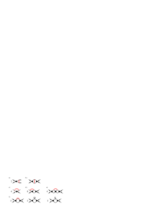
FIG. 13.: Leading order radiation pion graphs for $NN$ scattering. The wavy lines are radiation pions and $\delta M$, $\delta Z$ are the mass and field renormalization counterterms. There is a further field renormalization contribution that is included in Eq. (C30).

It is instructive to look at the result of evaluating some of these diagrams:

$$a) = -3i{\cal A}_{-1}{g_{A}^{2}m_{\pi}^{2}\over(4\pi f)^{2}}\bigg{[}{1\over\epsilon}-{5\over 3}-{\rm ln}\Big{(}{m_{\pi}^{2}\over{\overline{\mu}}^{2}}\Big{)}\bigg{]}\,,$$ (C24)

$$b) = [{\cal A}_{-1}]\,^{2}\,{g_{A}^{2}Mm_{\pi}^{2}\over(4\pi f)^{2}}\,\Bigg{\{}{3\,p\over 4\pi}\,\bigg{[}{1\over\epsilon}+{1\over 3}-2\,{\rm ln}\,2-{\rm ln}\Big{(}{m_{\pi}^{2}\over{\overline{\mu}}^{2}}\Big{)}-{\rm ln}\Big{(}{-p^{2}\over{\overline{\mu}}^{2}}\Big{)}\bigg{]}$$ (C26)

$$\qquad\qquad\qquad\qquad+{i\sqrt{Mm_{\pi}}\over 4\sqrt{\pi}}\,I_{1}\Big{(}{E\over m_{\pi}}\Big{)}\Bigg{\}}\,,$$

$$c) = {ig_{A}^{2}\over\sqrt{\pi}f^{2}}\Big{(}{m_{\pi}\over M}\Big{)}^{3/2}I_{2}\Big{(}{E\over m_{\pi}}\Big{)}\,,$$ (C27)

where $\bar{\mu}^{2}=\pi e^{-\gamma_{E}}\mu^{2}$, and $I_{1}$ and $I_{2}$ are hypergeometric functions given in Ref. [29]. The $1/\epsilon$ poles are cancelled by insertions of a $D_{2}m_{\pi}^{2}$ counterterm. The leading order amplitude ${\cal A}_{-1}\sim 1/(Mp)$, so we see that Eq. (C24) has terms proportional to

$$\left({m_{\pi}\over M}\right)^{3/2}\!\!\!\!\!\!,\qquad{m_{\pi}^{2}\over Mp}\qquad{\rm and}\qquad{m_{\pi}^{5/2}\over M^{1/2}p^{2}}\,.$$ (C28)

For $p\sim Q_{r}$ these terms scale as $Q_{r}^{3}/M^{3}$, as anticipated by the power counting. At $p\sim m_{\pi}\sim Q$, these terms scale like $(Q/M)^{3/2},Q/M$, and $(Q/M)^{1/2}$ respectively. The graphs which give rise to the $Q^{1/2}(Q)$ corrections have two (one) external bubble sums. By external bubble sums we mean bubble sums that do not appear inside radiation loops. External bubble sums go like $1/p$, which scales like $1/Q_{r}$ at $p\sim Q_{r}$ but $1/Q$ at $p\sim m_{\pi}$. So for each external bubble sum, the graph picks up an additional $Q_{r}/Q\sim Q^{-1/2}$ upon scaling from $p\sim Q_{r}$ to $p\sim m_{\pi}$. Terms which scale like $Q^{1/2}$ at $p\sim m_{\pi}$ are actually larger than NNLO in the $Q$ counting. The $Q^{1/2}$ contributions come from graphs $b),e)$ and $f)$, and cancel when these graphs are added together.

In the ${}^{1}S_{0}$ channel the sum of all $Q_{r}^{3}$ graphs in Fig. 13 is [29]:

$$i\,{\cal A}_{3}^{rad} = 6i\,[{\cal A}_{-1}]^{2}{g_{A}^{2}m_{\pi}^{2}\over(4\pi f)^{2}}\,\left({1\over C_{0}^{(^{1}S_{0})}}-{1\over C_{0}^{(^{3}S_{1})}}\right)\,\bigg{[}\frac{1}{3}+{\rm ln}\Big{(}{{\mu}^{2}\over m_{\pi}^{2}}\Big{)}\bigg{]}$$ (C30)

$$+i\,[{\cal A}_{-1}]^{2}\left({1\over C_{0}^{(^{1}S_{0})}}-{1\over C_{0}^{(^{3}S_{1})}}\right)^{2}{g_{A}^{2}\over\sqrt{\pi}f^{2}}\Big{(}{m_{\pi}\over M}\Big{)}^{3/2}I_{2}\Big{(}{E\over m_{\pi}}\Big{)}\,,$$

where the $\ln(\mu)$ dependence in Eq. (C30) is cancelled by a $\ln(\mu)$ in $D_{2}^{(^{1}S_{0})}(\mu)$. The sum of the $Q_{r}^{3}$ diagrams turns out to be much smaller than anticipated by the power counting. For $p\sim Q_{r}$, the first term is suppressed by a factor of $\sim 1/Q_{r}[1/a^{(^{1}S_{0})}-1/a^{(^{3}S_{1})}]$, the second by $\sim 1/Q_{r}^{2}[1/a^{(^{1}S_{0})}-1/a^{(^{3}S_{1})}]^{2}$. This suppression occurs because the radiation pions couple to a charge of Wigner’s $SU(4)$ symmetry[22], which is a symmetry of the leading order Lagrangian in the limit $a^{(^{1}S_{0})},a^{(^{3}S_{1})}\rightarrow\infty$ (or $a^{(^{1}S_{0})}=a^{(^{3}S_{1})}$)[23]. The order $Q_{r}^{3}$ radiation pion graphs are therefore a small correction to the S-wave scattering amplitude. Furthermore, to order $Q$ the $Q_{r}^{3}$ graphs simply give an additional contribution to the $\zeta_{3}$ constant that appears in Eqs. (45),

$$\zeta_{3}^{(3)}=-6\,{g_{A}^{2}\over(4\pi f)^{2}}\,\left({1\over C_{0}^{(^{1}S_{0})}}-{1\over C_{0}^{(^{3}S_{1})}}\right)\bigg{[}{1\over 3}+{\rm ln}\Big{(}{\mu^{2}\over m_{\pi}^{2}}\Big{)}\bigg{]}\,.$$ (C31)

The $\mu$ dependence in $\zeta_{3}^{(3)}$ is cancelled by $\mu$ dependence in $D_{2}^{(^{1}S_{0})}$. The result in the ${}^{3}S_{1}$ channel is obtained from Eqs. (C30) and (C31) by switching the ${}^{1}S_{0}$ and ${}^{3}S_{1}$ labels.

3 Scaling radiation contributions from $Q_{r}$ to $m_{\pi}$

Since we are interested in the power counting for $p\sim m_{\pi}$ it is important to know how big a radiation pion graph may get when $p$ is lowered from $Q_{r}$ to $m_{\pi}$. The $Q_{r}^{3}$ graphs have pieces that scale as $Q^{1/2},Q$, $Q^{3/2},\ldots$, for $p\sim m_{\pi}$ as discussed in the previous section. In order to know which radiation pion graphs to include at a given order in the KSW power counting, we must know the size of the leading term in the $Q$ expansion of a $Q_{r}^{k}$ graph for $p\sim m_{\pi}$. In this section we will prove that an order $Q_{r}^{k}$ calculation is sufficient to determine the order $Q^{k/2-1}$ result.

To see this first consider the $Q$ expansion of $p\,{\rm cot}\,\delta$ in the ${}^{1}S_{0}$ channel:

$$p\,{\rm cot}\,\delta = ip+{4\pi\over M}{1\over{\cal A}}$$ (C32)

$$= ip+{4\pi\over M}{1\over{\cal A}_{-1}}-{4\pi\over M}{{\cal A}_{0}\over[{\cal A}_{-1}]^{2}}-{4\pi\over M}\left({{\cal A}_{1}\over[{\cal A}_{-1}]^{2}}-{{\cal A}_{0}^{2}\over[{\cal A}_{-1}]^{3}}\right)$$ (C34)

$$-{4\pi\over M}\left({{\cal A}_{2}\over[{\cal A}_{-1}]^{2}}-{2{\cal A}_{0}{\cal A}_{1}\over[{\cal A}_{-1}]^{3}}+{{\cal A}_{0}^{3}\over[{\cal A}_{-1}]^{4}}\right)+\dots\,.$$

$p\,{\rm cot}\,\delta$ is real and an analytic function of $p^{2}$ near $p=0$. This will be true order by order in $Q$ so:

$${{\cal A}_{0}\over[{\cal A}_{-1}]^{2}}=f_{0}\, \Rightarrow \,{\cal A}_{0}=f_{0}[{\cal A}_{-1}]^{2}\,,$$ (C35)

$${{\cal A}_{1}\over[{\cal A}_{-1}]^{2}}-{[{\cal A}_{0}]^{2}\over[{\cal A}_{-1}]^{3}}=f_{1}\, \Rightarrow \,{\cal A}_{1}=f_{1}[{\cal A}_{-1}]^{2}+f_{0}^{2}[{\cal A}_{-1}]^{3}\,,$$ (C36)

$${{\cal A}_{2}\over[{\cal A}_{-1}]^{2}}-{2{\cal A}_{0}{\cal A}_{1}\over[{\cal A}_{-1}]^{3}}+{[{\cal A}_{0}]^{3}\over[{\cal A}_{-1}]^{4}}=f_{2}\, \Rightarrow \,{\cal A}_{2}=f_{2}[{\cal A}_{-1}]^{2}+2f_{0}f_{1}[{\cal A}_{-1}]^{3}+f_{0}^{3}[{\cal A}_{-1}]^{4}\,,$$ (C37)

where the $f_{k}$ are real functions of $p$ which are analytic about $p^{2}=0$. The general form of a higher order amplitude is powers of ${\cal A}_{-1}$ multiplied by functions of $p$. The crucial point is that the function multiplying the $[{\cal A}_{-1}]^{2}$ is the only new contribution. The coefficient of $[{\cal A}_{-1}]^{m}$, $m>2$, is determined by lower order amplitudes. The graphs giving the $m>2$ contributions are “$C_{0}$ reducible” by which we mean that they fall apart when cut at an ${\cal A}_{-1}$ vertex.

This generalizes to the $Q_{r}$ expansion of radiation pion graphs, the only difference being that the radiation pion contribution starts out at $Q_{r}^{3}$, while the potential pion starts out at $Q^{0}$. A $Q_{r}^{k}$ radiation pion correction to the amplitude will be of the form:

$${\cal A}_{k}=[{\cal A}_{-1}]^{2}f_{k,2}+[{\cal A}_{-1}]^{3}f_{k,3}+\ldots+[{\cal A}_{-1}]^{k-1}f_{k,k-1}.$$ (C38)

Again, the $f_{k,m}$ are real and analytic about $p^{2}=0$ and all the $f_{k,m}$ except for $f_{k,2}$ will be determined from lower order amplitudes. Since ${\cal A}_{k}\sim Q_{r}^{k}$ and ${\cal A}_{-1}\sim 1/(Mp)$, $f_{k,2}\sim Q_{r}^{k+2}$ for $p\sim Q_{r}$. To understand how $f_{k,2}$ scales with $Q$ as $p$ is lowered to $m_{\pi}$, note that without loss of generality, $f_{k,2}$ can be written as

$$f_{k,2}={({\sqrt{Mm_{\pi}}})^{k+2}\over\Lambda_{\chi}^{2}\ {\overline{\Lambda}}^{\>k-2}}\ {\hat{f}}_{k,2}\left({p\over\sqrt{Mm_{\pi}}},\ldots\right)\,,$$ (C39)

where the ellipses denote momentum dependence that involves scales other than $Q_{r}$, and ${\overline{\Lambda}}=\Lambda_{\chi}$, $\Lambda$, or $M$. For $p\sim m_{\pi}$ the ellipse denote dependence on the dimensionless variables $p/m_{\pi}$, $ap$, and $p/\,{\overline{\Lambda}}$. For $p\sim m_{\pi}$, ${p/\sqrt{Mm_{\pi}}}\sim(Q/M)^{1/2}$ and the function ${\hat{f}}_{k,2}$ can be expanded in its first argument:

$${\cal A}_{-1}^{2}f_{k,2}={\cal A}_{-1}^{2}{({\sqrt{Mm_{\pi}}})^{k+2}\over\Lambda_{\chi}^{2}\ {\overline{\Lambda}}^{\>k-2}}{\hat{f}}_{k,2}\left(0,\ldots\right)\left[1+O\left({Q\over M}\right)^{1/2}\right]\,.$$ (C40)

Therefore, the new contribution at $Q_{r}^{k}$ scales like $Q^{k/2-1}$ (plus subleading terms) for $p\sim m_{\pi}$. This is consistent with the result of the $Q_{r}^{3}$ calculation, where the largest contributions from individual graphs scaled as $Q^{1/2}$. A cancellation between graphs resulted in this contribution vanishing. The remaining terms scale as $Q$, $Q^{3/2},\ldots$.

Next we consider contributions to the amplitude from $C_{0}$ reducible graphs. If a $C_{0}$ reducible graph is obtained by joining $j$ $C_{0}$ irreducible graphs where the $j$’th graph scales as $Q^{\alpha_{j}}$ at $p\sim m_{\pi}$, then the $C_{0}$ reducible graph scales as

$$Q^{\,j-1+\sum_{i=1}^{j}\alpha_{i}}\,.$$ (C41)

For example, the order $Q_{r}^{4}$ graphs in Fig. 14 are each obtained by joining a $Q^{0}$ potential pion graph with a $Q_{r}^{3}$ radiation pion graph. The radiation graphs scale as $Q^{1/2}$ for $p\sim m_{\pi}$ so the individual graphs in Fig.[14] scale as $Q^{3/2}$ for $p\sim m_{\pi}$. No $C_{0}$ irreducible graphs give an order $Q$ contribution.

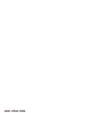
FIG. 14.: Example of order $Q_{r}^{4}$ graphs that have three external bubble sums.

Since $Q^{k/2-1}=Q$ for $k=4$, the $Q_{r}^{4}$ radiation pion graphs can have a contribution that is NNLO for $p\sim m_{\pi}$. This calculation is taken up in the next section. Note that a calculation of the order $Q_{r}^{5}$ graphs would be necessary to determine the order $Q^{3/2}$ terms.

4 The order $Q$ part of the order $Q_{r}^{4}$ radiation pion graphs

The order $Q_{r}^{4}$ radiation pion contributions come from graphs that have one radiation pion, an arbitrary number of $C_{0}$’s, and one insertion of a $C_{2}p^{2}$, $D_{2}m_{\pi}^{2}$, or $G_{2}$ operator or one potential pion. The coefficient $G_{2}$ multiplies a four-nucleon operator that couples to the axial pion current,

$${\cal L}=\frac{i}{2}\,G_{2}\,[N^{T}P^{(s)}_{i}N]^{\dagger}\,[N^{T}P^{(s)}_{i}\sigma_{j}(\xi\partial_{j}\xi^{\dagger}-\xi^{\dagger}\partial_{j}\xi)N]+h.c.\,.$$ (C42)

Note that due to the hermitian conjugate this operator is the same for $s=\!^{1}S_{0}$ and $s=\!^{3}S_{1}$. Power counting these graphs gives $Q_{r}^{4}/(M^{3}\Lambda_{\chi}^{2}\Lambda)$, i.e. they are suppressed by $Q_{r}/\Lambda$ relative to the leading radiation pion graphs in Fig. 13. Note that $Q_{r}=360\,{\rm MeV}$, so for $\Lambda<360\,{\rm MeV}$, the $Q_{r}/\Lambda$ expansion does not converge. If this is the case then the radiation pion contribution is not calculable. This is true of radiation contributions even when we scale down to $p\sim m_{\pi}$. To make the radiation contributions calculable we must have a power counting for the pure potential contributions that works for $p\sim Q_{r}$. One possible resolution is to ignore radiation pion contributions since at low momenta the radiation pions can be integrated out. However, this makes the coefficients of four nucleon operators depend on $m_{\pi}$ in a non-trivial way. We will proceed by computing the radiation contribution which is formally order $Q$ in both S-wave channels even though the size of the spin triplet potential diagrams in section III B indicate that a modification of the power counting is likely necessary to obtain a convergent expansion in this channel. Since the $C_{2}p^{2}$ and $D_{2}m_{\pi}^{2}$ operators and potential pion exchange do not respect Wigner symmetry, there will be no suppression by factors of $1/(a\,Q_{r})$ at this order.

For calculational purposes it is useful to define offshell amplitudes for S-wave transitions, $N(p_{1})N(p_{2})\to N(p_{3})N(p_{4})$, induced by 4-nucleon operators. These amplitudes are equal to a sum of Feynman diagrams where the equations of motion have not been used. They can be treated as vertices and inserted inside loop graphs, which greatly reduces the number of order $Q_{r}^{4}$ diagrams. The offshell order $1/Q$ amplitude in $n$ dimensions is

$$i\,{\cal A}^{(-1)} = \quad\begin{picture}(15.0,10.0)(1.0,1.0)\put(1.0,3.0){\line(1,1){10.0}} \put(1.0,3.0){\line(1,-1){10.0}} \put(1.0,3.0){\line(-1,1){10.0}} \put(1.0,3.0){\line(-1,-1){10.0}} \put(-4.0,15.0){\mbox{$C_{0}$}} \end{picture}+\quad\ \begin{picture}(15.0,10.0)(1.0,1.0)\put(1.0,3.0){\line(-1,1){10.0}} \put(1.0,3.0){\line(-1,-1){10.0}} \put(11.0,3.0){\circle{20.0}} \put(21.0,3.0){\line(1,1){10.0}} \put(21.0,3.0){\line(1,-1){10.0}} \put(-6.0,18.0){\mbox{$C_{0}$}} \put(14.0,18.0){\mbox{$C_{0}$}} \end{picture}\qquad+\,\ldots\ =\qquad\begin{picture}(15.0,10.0)(1.0,1.0)\put(4.0,3.0){\line(1,1){10.0}} \put(4.0,3.0){\line(1,-1){10.0}} \put(1.0,3.0){\circle*{8.0}} \put(-2.0,3.0){\line(-1,1){10.0}} \put(-2.0,3.0){\line(-1,-1){10.0}} \end{picture}\ \ =\ -\frac{4\pi i}{M}\>\frac{1}{\gamma-\tau(-M\bar{E}-i\epsilon)^{n/2-1}}\,,$$ (C44)

where

$$\gamma=\frac{4\pi}{MC_{0}(\mu)}+\mu\,,\qquad\tau=-\,{\Gamma(1-n/2)\over(4\pi)^{n/2-1}}\Big{(}\frac{\mu}{2}\Big{)}^{3-n}\,,$$ (C45)

and $\bar{E}$ is the center of mass energy

$$\bar{E}=E_{1}+E_{2}-{({\vec{p}}_{1}+{\vec{p}}_{2})^{2}\over 4M}=E_{3}+E_{4}-{({\vec{p}}_{3}+{\vec{p}}_{4})^{2}\over 4M}\,.$$ (C46)

At order $Q^{0}$ the NN amplitude has contributions from the four nucleon operators $C_{2}$, $D_{2}$, and $C_{0}^{(0)}$. In $n$ dimensions the offshell amplitude for $C_{2}$ graphs is

$$i\,{\cal A}_{C_{2}} = \quad\begin{picture}(15.0,10.0)(1.0,1.0)\put(1.0,3.0){\line(1,1){10.0}} \put(1.0,3.0){\line(1,-1){10.0}} \put(1.0,3.0){\line(-1,1){10.0}} \put(1.0,3.0){\line(-1,-1){10.0}} \put(-4.0,15.0){\mbox{$C_{2}$}} \end{picture}+\quad\ \begin{picture}(15.0,10.0)(1.0,1.0)\put(-5.0,3.0){\line(-1,1){10.0}} \put(-5.0,3.0){\line(-1,-1){10.0}} \put(11.0,3.0){\circle{20.0}} \put(21.0,3.0){\line(1,1){10.0}} \put(21.0,3.0){\line(1,-1){10.0}} \put(-2.0,3.0){\circle*{8.0}} \put(14.0,18.0){\mbox{$C_{2}$}} \end{picture}\qquad+\quad\ \begin{picture}(15.0,10.0)(1.0,1.0)\put(1.0,3.0){\line(-1,1){10.0}} \put(1.0,3.0){\line(-1,-1){10.0}} \put(11.0,3.0){\circle{20.0}} \put(27.0,3.0){\line(1,1){10.0}} \put(27.0,3.0){\line(1,-1){10.0}} \put(-6.0,18.0){\mbox{$C_{2}$}} \put(24.0,3.0){\circle*{8.0}} \end{picture}\qquad+\quad\ \begin{picture}(15.0,10.0)(1.0,1.0)\put(-5.0,3.0){\line(-1,1){10.0}} \put(-5.0,3.0){\line(-1,-1){10.0}} \put(11.0,3.0){\circle{20.0}} \put(31.0,3.0){\circle{20.0}} \put(47.0,3.0){\line(1,1){10.0}} \put(47.0,3.0){\line(1,-1){10.0}} \put(-2.0,3.0){\circle*{8.0}} \put(44.0,3.0){\circle*{8.0}} \put(14.0,18.0){\mbox{$C_{2}$}} \end{picture}$$ (C48)

$$= -i\,\frac{C_{2}}{(C_{0})^{2}}\>M\bar{E}\ \Big{[}{\cal A}^{(-1)}\,\Big{]}^{2}+i\,\frac{C_{2}}{C_{0}}\>\bigg{\{}\frac{({\vec{p}}_{1}-{\vec{p}}_{2})^{2}+({\vec{p}}_{3}-{\vec{p}}_{4})^{2}}{8}-M\bar{E}\bigg{\}}\ {\cal A}^{(-1)}\,.$$ (C49)

Note that $C_{2}(\mu)/C_{0}(\mu)$ and therefore the offshell $C_{2}$ amplitude are $\mu$ dependent. The onshell amplitude is $\mu$ independent using the order $1/Q^{2}$ part of the beta function in Eq. (19) since the term proportional to $C_{2}/C_{0}$ vanishes by the equations of motion. The offshell amplitude that includes the graphs with $D_{2}$ or $C_{0}^{(0)}$ vertices is

$$i\,{\cal A}_{D_{2}} = \quad\begin{picture}(15.0,10.0)(1.0,1.0)\put(1.0,3.0){\line(1,1){10.0}} \put(1.0,3.0){\line(1,-1){10.0}} \put(1.0,3.0){\line(-1,1){10.0}} \put(1.0,3.0){\line(-1,-1){10.0}} \put(-12.0,20.0){\mbox{$D_{2}$,$C_{0}^{(0)}$}} \end{picture}+\quad\ \begin{picture}(15.0,10.0)(1.0,1.0)\put(-5.0,3.0){\line(-1,1){10.0}} \put(-5.0,3.0){\line(-1,-1){10.0}} \put(11.0,3.0){\circle{20.0}} \put(21.0,3.0){\line(1,1){10.0}} \put(21.0,3.0){\line(1,-1){10.0}} \put(-2.0,3.0){\circle*{8.0}} \put(6.0,22.0){\mbox{$D_{2}$,$C_{0}^{(0)}$}} \end{picture}\qquad+\quad\ \begin{picture}(15.0,10.0)(1.0,1.0)\put(1.0,3.0){\line(-1,1){10.0}} \put(1.0,3.0){\line(-1,-1){10.0}} \put(11.0,3.0){\circle{20.0}} \put(27.0,3.0){\line(1,1){10.0}} \put(27.0,3.0){\line(1,-1){10.0}} \put(-14.0,22.0){\mbox{$D_{2}$,$C_{0}^{(0)}$}} \put(24.0,3.0){\circle*{8.0}} \end{picture}\qquad+\quad\ \begin{picture}(15.0,10.0)(1.0,1.0)\put(-5.0,3.0){\line(-1,1){10.0}} \put(-5.0,3.0){\line(-1,-1){10.0}} \put(11.0,3.0){\circle{20.0}} \put(31.0,3.0){\circle{20.0}} \put(47.0,3.0){\line(1,1){10.0}} \put(47.0,3.0){\line(1,-1){10.0}} \put(-2.0,3.0){\circle*{8.0}} \put(44.0,3.0){\circle*{8.0}} \put(6.0,22.0){\mbox{$D_{2}$,$C_{0}^{(0)}$}} \end{picture}\phantom{xxxxxxxxxxxxxx}$$ (C51)

$$= -i\,\bigg{[}\frac{D_{2}}{(C_{0})^{2}}\>m_{\pi}^{2}+\frac{C_{0}^{(0)}}{(C_{0})^{2}}\bigg{]}\ \Big{[}{\cal A}^{(-1)}\,\Big{]}^{2}\,,$$ (C52)

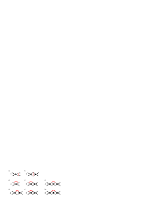
FIG. 15.: Order $Q_{r}^{4}$ radiation pion graphs with insertions of $C_{2}$ and $D_{2}$. The solid lines are nucleons and the wavy lines are radiation pions. The black circle denotes the $C_{0}$ bubble sum, $i{\cal A}^{(-1)}$, and the hatched circle denotes an insertion of $i{\cal A}_{C_{2}}$ or $i{\cal A}_{D_{2}}$ given in Eqs. (LABEL:offC2) and (LABEL:offD2).

The order $Q_{r}^{4}$ radiation pion graphs with insertions of $i{\cal A}_{C_{2}}$ or $i{\cal A}_{D_{2}}$ are shown in Fig. 15. We find that graphs with insertions of $i{\cal A}_{D_{2}}$ give contributions that are order $Q^{2}$ or higher. The graphs which have an $i{\cal A}_{D_{2}}$ external to the radiation loop (Fig.15b,f,h) have no order $Q$ contribution because the same cancellation that occurs in Fig. 13b,e,f occurs here. Of the remaining graphs only Fig. 15e with two external bubble sums can have an order $Q$ contribution, however inside the radiation pion loop $i{\cal A}_{D_{2}}\sim m_{\pi}^{2}/Q_{r}^{2}\sim Q$ (not $Q^{0}$) so this graph is order $Q^{2}$.

With insertions of $i{\cal A}_{C_{2}}$, the only graphs in Fig. 15 which do not give an order $Q$ contribution are a) and c). Diagrams d) and g) give a non-zero order $Q$ contribution even though they have only one external bubble sum. The order $Q$ contribution comes from the $\mu$ dependent part of $i{\cal A}_{C_{2}}$. Since these $Q_{r}^{4}$ graphs have one external bubble sum they are expected to be $\sim Q^{3/2}$. However, with $(\vec{p}_{1}-\vec{p}_{2})^{2}\sim Q_{r}^{2}$ or $M\bar{E}\sim Q_{r}^{2}$, and $\mu\sim Q$ the $\mu$ dependent part of $i{\cal A}_{C_{2}}$ is order $Q_{r}/\mu\sim 1/\sqrt{Q}$. This extra factor makes these graphs order $Q$. For the ${}^{1}S_{0}$ channel, the sum of the order $Q$ contributions from the $C_{2}$ radiation graphs in Fig. 15 is

$$i{\cal A}^{rad}_{C_{2}}=\frac{ig_{A}^{2}}{f^{2}}\Big{[}{\cal A}_{-1}^{(^{1}S_{0})}\Big{]}^{2}\,{Mm_{\pi}^{2}(m_{\pi}-\mu)\over 4\pi}\Bigg{\{}\frac{C_{2}^{(^{1}S_{0})}}{[C_{0}^{(^{1}S_{0})}]^{2}}+\frac{C_{2}^{(^{3}S_{1})}}{[C_{0}^{(^{3}S_{1})}]^{2}}-{C_{2}^{(^{1}S_{0})}+C_{2}^{(^{3}S_{1})}\over C_{0}^{(^{1}S_{0})}C_{0}^{(^{3}S_{1})}}\Bigg{\}}\,.$$ (C53)

The corresponding amplitude in the ${}^{3}S_{1}$ channel is obtained by exchanging the ${}^{1}S_{0}$ and ${}^{3}S_{1}$ labels in Eq. (C53).

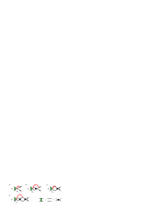
FIG. 16.: Order $Q_{r}^{4}$ radiation pion graphs with insertions of $G_{2}$.

The result in Eq. (C53) is $\mu$ dependent. For the term proportional to $m_{\pi}^{2}$ the $\mu$ dependence is cancelled by a radiation contribution to the beta function for $D_{2}(\mu)$. The $\mu$ dependence of the $m_{\pi}^{3}$ term is cancelled by $G_{2}(\mu)$. To calculate the PDS beta function for $G_{2}(\mu)$ we consider graphs with $G_{2}$ dressed with $C_{0}^{(^{1}S_{0})}$ bubbles on one side and $C_{0}^{(^{3}S_{1})}$ bubbles on the other. We also consider graphs with a $C_{2}$ vertex next to a $NN\pi$ vertex:

(C54)

When the derivatives in ${\cal O}_{2}$ act on the nucleons on the right there is a piece in which the numerator cancels the propagator exactly. This piece has the same form as a $NNNN\pi$ vertex and contributes to the beta function for $G_{2}$ when dressed with $C_{0}$ bubbles. We find

$$\beta_{G_{2}} = {\mu M\over 4\pi}\,G_{2}(C_{0}^{(^{1}S_{0})}+C_{0}^{(^{3}S_{1})})$$ (C57)

$$+{g_{A}\mu M^{2}\over 4\pi}\Big{[}C_{0}^{(^{1}S_{0})}C_{2}^{(^{1}S_{0})}+C_{0}^{(^{3}S_{1})}C_{2}^{(^{3}S_{1})}-C_{0}^{(^{3}S_{1})}C_{2}^{(^{1}S_{0})}-C_{0}^{(^{1}S_{0})}C_{2}^{(^{3}S_{1})}\Big{]}\,,$$

which has the solution

$$G_{2}(\mu)=\kappa_{G}\frac{MC_{0}^{(^{1}S_{0})}}{4\pi}\frac{MC_{0}^{(^{3}S_{1})}}{4\pi}+g_{A}M\,[C_{2}^{(^{1}S_{0})}+C_{2}^{(^{3}S_{1})}]\,,$$ (C58)

with $\kappa_{G}$ the constant of integration. Eq. (C58) gives $G_{2}(\mu)\sim 1/\mu^{2}$. Because $G_{2}$ is the coefficient of the four nucleon coupling to the axial current it has the same renormalization group equation as the weak axial four nucleon operator considered in Ref. [13]. Using the scaling of $G_{2}$ to power count the diagrams in Fig. 16 we find that they are order $Q_{r}^{4}$ radiation pion graphs. For the ${}^{1}S_{0}$ channel, the sum of the order $Q$ part of the diagrams in Fig. 16 is

$$i\,{\cal A}_{G_{2}}^{rad}=\frac{ig_{A}}{f^{2}}[A_{-1}^{(^{1}S_{0})}]^{2}\frac{G_{2}}{C_{0}^{(^{1}S_{0})}C_{0}^{(^{3}S_{1})}}{m_{\pi}^{2}(m_{\pi}-\mu)\over 4\pi}\,.$$ (C59)

The result in the ${}^{3}S_{1}$ channel is obtained by interchanging the labels ${}^{1}S_{0}$ and ${}^{3}S_{1}$. Using Eq. (C58) we see that the $\mu$ dependence of the $m_{\pi}^{3}$ term in Eq. (C53) is cancelled by the $m_{\pi}^{3}$ term in Eq. (C59). The $\mu$ dependence of the $m_{\pi}^{2}$ term in Eq. (C59) is again cancelled by $D_{2}(\mu)$.

The final order $Q_{r}^{4}$ diagrams that we must consider are those with one potential pion, one radiation pion and an arbitrary number of $C_{0}$’s shown in Fig. 17.

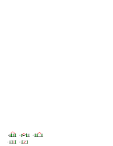
FIG. 17.: Order $Q_{r}^{4}$ radiation pion graphs with one potential pion.

Here we find that only graphs with two external bubble sums can give an order $Q$ contribution. Graphs in Fig. 17 with three external bubbles sums are $C_{0}$ reducible and do not give order $Q$ contributions. Furthermore, of all the diagrams in Fig. 17 with two external bubble sums only the three shown in Fig. 18 give an order $Q$ contribution.

FIG. 18.: The three order $Q_{r}^{4}$ radiation pion graphs with one potential pion that give an order $Q$ contribution for $p\sim m_{\pi}$.

These are the graphs in which the potential pion exchange is inside the radiation pion loop. This ensures that all potential loop momenta in the graph see the scale $Q_{r}$ which is necessary for the graph to give an order $Q$ contribution. So, for example, we find that the graph in Fig. 19 does not give an order $Q$ contribution. The diagrams in Fig. 18 look somewhat daunting since they involve a three, four, and five loop calculation. Nevertheless, their order $Q$ contribution can be evaluated analytically.

FIG. 19.: An order $Q_{r}^{4}$ radiation pion graphs with one potential pion that does not give an order $Q$ contribution.

Adding up the the order $Q$ part of the diagrams in Fig. 18 gives

$$i\,{\cal A}^{rad}_{\pi}=i\,\frac{5}{3}\,\Big{(}\frac{g_{A}^{2}}{2f^{2}}\Big{)}^{2}\,\frac{Mm_{\pi}^{3}}{4\pi}\Big{(}\frac{MA_{-1}}{4\pi}\Big{)}^{2}\,.$$ (C60)

It is interesting that the order $Q$ part of these graphs is not multiplied by a nontrivial function of $p/m_{\pi}$. At one higher order, $Q^{3/2}$, the diagrams in Fig. 17 will give a result which involves a function of $p/m_{\pi}$.

The results in Eqs. (C53,C59,C60) give the complete order $Q$ contribution from order $Q_{r}^{4}$ graphs. It is interesting to note that all contributions are equal to a constant times $[{\cal A}_{-1}]^{2}$. Therefore they simply give an additional contribution to the constant $\zeta_{3}$ that appears in Eqs. (45) and (81),

$$\zeta_{3}^{(4)} = -\frac{5}{3}\,\Big{(}\frac{M}{4\pi}\Big{)}^{2}\>\Big{(}\frac{g_{A}^{2}}{2f^{2}}\Big{)}^{2}\>\frac{Mm_{\pi}}{4\pi}$$ (C62)

$$-\frac{(m_{\pi}-\mu)g_{A}}{4\pi f^{2}}\Bigg{\{}\frac{G_{2}-Mg_{A}(C_{2}^{(^{1}S_{0})}+C_{2}^{(^{3}S_{1})})}{C_{0}^{(^{1}S_{0})}C_{0}^{(^{3}S_{1})}}+Mg_{A}\Bigg{(}\>\frac{C_{2}^{(^{1}S_{0})}}{[C_{0}^{(^{1}S_{0})}]^{2}}+\frac{C_{2}^{(^{3}S_{1})}}{[C_{0}^{(^{3}S_{1})}]^{2}}\>\Bigg{)}\Bigg{\}}\,.$$

The result for $\zeta_{3}^{(4)}$ is the same in the ${}^{3}S_{1}$ channel. The $\mu$ dependence in $\zeta_{3}^{(4)}$ is cancelled by $\mu$ dependence in $D_{2}$.

The complete order $Q$ contribution from radiation pion graphs is the sum of Eqs. (C31) and (C62):

$$\zeta_{3}^{rad}=\zeta_{3}^{(3)}+\zeta_{3}^{(4)}\,.$$ (C63)

The order $Q$ radiation pion contribution to the $D_{2}^{(^{1}S_{0})}$ beta function in Eq. (19) is

$$\beta_{D_{2}}^{rad} = 12\frac{g_{A}^{2}}{(4\pi f)^{2}}\Big{(}\frac{1}{C_{0}^{(^{1}S_{0})}}-\frac{1}{C_{0}^{(^{3}S_{1})}}\Big{)}\Big{[}\,C_{0}^{(^{1}S_{0})}\Big{]}^{2}$$ (C65)

$$-\frac{\mu g_{A}}{4\pi f^{2}}\Bigg{\{}\frac{G_{2}-Mg_{A}(C_{2}^{(^{1}S_{0})}+C_{2}^{(^{3}S_{1})})}{C_{0}^{(^{1}S_{0})}C_{0}^{(^{3}S_{1})}}+Mg_{A}\Bigg{(}\>\frac{C_{2}^{(^{1}S_{0})}}{[C_{0}^{(^{1}S_{0})}]^{2}}+\frac{C_{2}^{(^{3}S_{1})}}{[C_{0}^{(^{3}S_{1})}]^{2}}\>\Bigg{)}\Bigg{\}}\Big{[}\,C_{0}^{(^{1}S_{0})}\Big{]}^{2}\,.$$

The contribution to the $D_{2}^{(^{3}S_{1})}$ beta function in Eq. (26) is obtained by switching the spin singlet and triplet labels.

For a consistent radiation pion calculation at momenta $p\sim Q_{r}$ it would be necessary to keep all powers of $p/Q_{r}$ in computing the $Q_{r}^{4}$ diagrams. If the $Q_{r}/\Lambda$ expansion were convergent then the magnitude of this radiation contribution would be small; being down by $Q_{r}^{5}$ relative to the leading order amplitude. For $Q_{r}/\Lambda>1$ it is necessary to modify the power counting for the potential diagrams to increase the scale $\Lambda$ before the radiation pion power counting will yield a convergent series. Since diagrams with one radiation pion are suppressed by $m_{\pi}^{2}/\Lambda_{\chi}^{2}$ relative to any leading order amplitude these contributions are always likely to contribute at the few percent level.

REFERENCES

- [1] J.F. Donoghue, E. Golowich and B.R. Holstein, Dynamics of the Standard Model (Cambridge University Press,, 1992).
- [2] E. Jenkins and A. Manohar, UCSD-PTH-91-30; E. Jenkins and A. Manohar, Phys. Lett. B255 (1991) 558, ibid B 259 (1991) 353.
- [3] V. Bernard, N. Kaiser, and U. Meissner, Phys. Rev. Lett. 67 (1991) 1515; Phys. Lett. B 319 (1993) 269; Int. J. Mod. Phys. E4 (1995) 193.
- [4] S. Weinberg, Phys. Lett. B251 (1990) 288; Nucl. Phys. B363 (1991) 3;
- [5] C. Ordonez and U. van Kolck, Phys. Lett. B291 (1992) 459; C. Ordonez, L. Ray and U. van Kolck, Phys. Rev. Lett. 72 (1994) 1982; U. van Kolck, Phys. Rev. C49 (1994) 2932; G.P. Lepage, nucl-th/9706029; T-S. Park, K. Kubodera, D-P. Min and M. Rho, Nucl. Phys. A646 (1999) 83; D.R. Phillips and T.D. Cohen, nucl-th/9906091. See the review, U. van Kolck, nucl-th/9902015 and references therein.
- [6] C. Ordonez, L. Ray, and U. van Kolck, Phys. Rev. C53, (1996) 2086,
- [7] E. Epelbaum, W. Glockle, and U.G. Meissner, nucl-th/9910064,
- [8] D. B. Kaplan, M. J. Savage, and M. B. Wise, Phys. Lett. B424 (1998) 390,
- [9] D. B. Kaplan, M. J. Savage, and M. B. Wise, Nucl. Phys. B534 (1998) 329,
- [10] U. van Kolck, hep-ph/9711222,
- [11] N. Kaiser, R. Brockmann, and W. Weise, Nucl. Phys. A625 (1997) 758.
- [12] E. Epelbaum and U.-G. Meissner, nucl-th/9903046; X. Kong and F. Ravndal, hep-ph/9903523; Phys. Lett. B450, (1999) 320; X. Kong and F. Ravndal, nucl-th/9902064; nucl-th/9904066; D. B. Kaplan, M. J. Savage, and M. B. Wise, Phys. Rev. C59 (1999) 617; J.-W. Chen et.al., Nucl. Phys. A644 (1998) 221; M. J. Savage, K. A. Scaldeferri, and M. B. Wise, nucl-th/9811029; J.-W. Chen, G. Rupak, and M. J. Savage, nucl-th/9905002; J.-W. Chen, H. W. Griesshammer, M. J. Savage, and R. P. Springer, Nucl. Phys. A644, 245 (1998); J.-W. Chen, nucl-th/9810021; D. B. Kaplan, M. J. Savage, R. P. Springer, and M. B. Wise, Phys. Lett. B449 (1999) 1; M. J. Savage and R. P. Springer, Nucl. Phys. A644 (1998) 235; P.F. Bedaque and H.W. Griesshammer, nucl-th/9907077,
- [13] Malcolm Butler and Jiunn-Wei Chen, nucl-th/9905059,
- [14] M. J. Savage, nucl-th/9905009, Proceedings of the INT Workshop on Nuclear Physics with Effective Field Theory, Seattle, WA 25-26 Feb 1999.
- [15] M. Binger, nucl-th/9901012,
- [16] G. Rupak and N. Shoresh, nucl-th/9902077,
- [17] G. Rupak and N. Shoresh, nucl-th/9906077,
- [18] T. Mehen and I. W. Stewart, nucl-th/9906010,
- [19] S. Fleming, T. Mehen amd I. Stewart, nucl-th/9906056.
- [20] V.G.J. Stoks, et.al., Phys. Rev. C48 (1993) 792; V.G.J. Stoks et.al., Phys. Rev. C49 (1994) 2950, nucl-th/9406039. (cf. http://nn-online.sci.kun.nl/NN/)
- [21] T. Mehen and I. W. Stewart, Phys. Rev. C59 (1999) 2365,
- [22] E. Wigner, Phys. Rev. 51, 106, 947 (1937).
- [23] T. Mehen, I. W. Stewart, and M. B. Wise, hep-ph/9902370,
- [24] J. Gegelia, nucl-th/9802038.
- [25] T. Mehen and I. W. Stewart, Phys. Lett. B445, (1999) 378,
- [26] M.C. Birse, J.A. McGovern, and K.G. Richardson, hep-ph/9807302.
- [27] I. W. Stewart, Ph.D. thesis, hep-ph/9907448.
- [28] J.-W. Chen, G. Rupak, and M. J. Savage, Nucl.Phys. A653 (1999) 386,
- [29] T. Mehen and I. W. Stewart, nucl-th/9901064,
- [30] J. Steele and D.B. Kaplan, nucl-th/9905027.
- [31] T.D. Cohen and J.M. Hansen, Phys. Rev. C59 (1999) 13; nucl-th/9901065.
- [32] D.B. Kaplan, private communication,
- [33] H.P. Stapp, T.J. Ypsilantis, and N. Metropolis, Phys. Rev. 105 (1957) 302,
- [34] N. Kaiser, S. Gerstendorfer, and W. Weise, Nucl. Phys. A637 (1998) 395,
- [35] J.W. Chen, G. Rupak, and M. J. Savage, nucl-th/9905002,
- [36] D.R. Phillips, G. Rupak, and M.J. Savage, nucl-th/9908054,
- [37] M. Luke and A. Manohar, Phys. Rev. D55 (1997) 4129,
- [38] P.F. Bedaque, H.W. Hammer and U. van Kolck, Nucl. Phys. A646, (1999) 444; P.F. Bedaque, H.W. Hammer and U. van Kolck, nucl-th/9906032. P.F. Bedaque and U. van Kolck, Phys. Lett. B428, (1998) 221; P.F. Bedaque, H.W. Hammer and U. van Kolck, Phys. Rev. C58, (1998) R641.
- [39] P.F. Bedaque and H.W. Griesshammer, nucl-th/9907077.
- [40] F.V. Tkachov, Phys. Lett. B100 (1981) 65; K.G. Chetyrkin and F.V. Tkachov, Nucl. Phys. B192 (1981) 159,
- [41] G. Passarino and M. Veltman, Nucl. Phys. B160 (1979) 151; G. Weiglein, R. Scharf, and M. Bohm, Nucl. Phys. B416 (1994) 606,
- [42] O.V. Tarasov, Phys. Rev. D54 (1996) 6479; Nucl. Phys. B502 (1997) 455.
- [43] R. Mertig and R. Scharf, Comput. Phys. Commun. 111 (1998) 265.
- [44] R. Harlander and M. Steinhauser, hep-ph/9812357,
- [45] E. Braaten and A. Nieto, Phys. Rev. D51, (1995) 6990.
- [46] A.K. Rajantie, Nucl. Phys. B480 (1996) 729.
- [47] M. Beneke and V.A. Smirnov, Nucl. Phys. B522 (1998) 321,
- [48] W.E. Caswell and G.P. Lepage, Phys. Lett. B167 (1986) 437; G.T. Bodwin, E. Braaten, and G.P. Lepage, Phys. Rev. D55 (1997) 1125.
- [49] B. Grinstein and I. Rothstein, Phys. Rev. D 57 (1998) 78; P. Labelle, Phys. Rev. D58 (1998) 093013; M. Luke, A.V. Manohar, and I.Z. Rothstein, hep-ph/9910209,
- [50] M. Luke and M.J. Savage, Phys. Rev. D57 (1998) 413;
- [51] H.W. Griesshammer, Phys. Rev. D58 (1998) 094027 and hep-ph/9810235,
- [52] H.W. Griesshammer, hep-ph/9804251,