Sum rules regarding the sign problem in Monte Carlo shell model calculations

Abstract

The Monte Carlo shell model is a powerful technique for computational nuclear structure. Only a certain class of nuclear interactions, however, such as pairing and quadrupole, are free of the numerical noise known as the sign problem. This paper presents sum rules that relate the sign problem to the $J=0$ pairing matrix elements, thus illuminating the extrapolation procedure routinely used for realistic shell-model interactions.

In recent years quantum Monte Carlo methods have become powerful numerical techniques for attacking the many-body problem in condensed matter, nuclear physics, and other fields. Unfortunately, these methods are also suceptible to what is known as the sign problem. Generically speaking, the sign problem arises when an expectation value to be computed is the average of a wildly fluctuating quantity, so that numerical noise overwhelms the signal.

This paper focuses on the auxiliary-field path integral, which is evaluated via Monte Carlo sampling, and further concentrates on the application to the nuclear shell model [1, 2, 3]. The nuclear shell model is an excellent venue for auxiliary-field Monte Carlo (AFMC) because one can prove that a large class of systems are free from the sign problem. The ‘goodness’ of an interaction with respect to the sign problem is related to the time-reversal properties of the effective one-body Hamiltonian [1].

This paper derives two sum rules for the time-reversal properties, and thus the sign-problem properties, of shell-model interactions. The sum rules are ultimately expressed in terms of the pairing matrix elements and prove two points of conventional, but previously unproved, wisdom in AFMC computations.

I Auxiliary-field Path Integrals

Traditional shell-model calculations diagonalize a Hamiltonian $\hat{H}$ in a many-body basis; the current best limit on model-space dimension is about $5\times 10^{8}$ [4] although more typical spaces have basis dimensions of $10^{5}$-$10^{7}$. Rather than diagonalization, AFMC shell model calculations employ the imaginary-time evolution operator $\exp(-\beta\hat{H})$ to project out the ground state and evaluate thermally weighted expectation values. For the purposes of this paper is it sufficient to sketch the broad outlines of the method; for a detailed description the interested reader is referred to [1, 3].

The nuclear Hamiltonian $\hat{H}$ is usually two-body and can be written as quadratic in one-body operators

$$\hat{H}=\sum_{\alpha}\epsilon_{\alpha}\hat{\rho}_{\alpha}+{1\over 2}\sum_{\alpha}V_{\alpha}\hat{\rho}_{\alpha}^{2}.$$ (1)

This is done in detail below. The quadratic term is source of all troubles; in order to facilitate numerical computation it is linearized, via the Hubbard-Stratonovich transformation, to form an effective one-body Hamiltonian that depends on the imaginary time $\tau$:

$$\hat{h}(\tau)=\sum_{\alpha}(\epsilon_{\alpha}+s_{\alpha}V_{\alpha}\sigma_{\alpha}(\tau))\hat{\rho}_{\alpha},$$ (2)

where $s_{\alpha}=\pm 1$ if $V_{\alpha}<0$ and $=\pm i$ if $V_{\alpha}>0$. Then the imaginary-time evolution operator $\exp(-\beta\hat{H})$ becomes a path-integral:

$$\exp(-\beta\hat{H})=\int{\cal D}[\sigma]\exp\left(-{1\over 2}\int_{0}^{\beta}d\tau\sum_{\alpha}|V_{\alpha}|^{2}\sigma_{\alpha}(\tau)^{2}\right)\left[{\cal T}\exp\left(-\int_{0}^{\beta}d\tau\hat{h}(\tau)\right)\right],$$ (3)

where ${\cal T}$ denotes time-ordering. This path integral can be evaluated by Monte Carlo sampling if a sufficiently well-behaved weight function $W(\sigma)$ can be found. An ideal weight function could be, for example, the trace of the integrand of Eqn. (3) itself. Unfortunately this choice of $W(\sigma)$ often takes on both positive and negative values and one must use $|W|$ as a weight function. In those cases typically $\left\langle W/|W|\right\rangle\ll 1$, and the statistical errors for the Monte Carlo value of the observable are overwhelmingly large. For AFMC methods this is the manifestation of the sign problem.

II Application to the spherical shell model

The shell model is built upon single-fermion states, using fermion creation and destruction operators $a^{\dagger},a$. For a spherical basis these fermion states have good angular momentum $j$ and $m$, as well as orbital angular momentum $\ell$ which dictates the parity $(-1)^{\ell}$. For each state we associate a “time-reversed” partner, $j$ and $-m$, and define a time-reversal operation by a bar: $\bar{a}_{j,m}=(-1)^{j+m+\ell}a_{j,-m}$ and $\bar{a}^{\dagger}_{j,m}=(-1)^{j+m+\ell}a^{\dagger}_{j,-m}$. Because of the half-spin statistics, $\bar{\bar{a}}_{j,m}=-a_{j,m}$. As hinted above, the time-reversal properties play a central role.

The two-body Hamiltonian is usually written as

$$\hat{H}_{2}={1\over 4}\sum_{abcd}\zeta_{ab}\zeta_{cd}\sum_{JT}\sum_{MT_{z}}V_{JT}(ab,cd)\hat{A}^{\dagger}_{JT,MT_{z}}(ab)\hat{A}_{JT,MT_{z}}(cd),$$ (4)

where $\zeta_{ab}\equiv\sqrt{1+\delta_{ab}}$, the $V_{JT}$ are matrix elements of the interaction, and the two-body creation operator is $\hat{A}^{\dagger}_{JT,MT_{z}}(ab)=\left[a^{\dagger}_{j_{a}}\otimes a^{\dagger}_{j_{b}}\right]_{JT,MT_{z}}$. Peforming a Pandya transformation from the particle-particle to the particle-hole representation, the Hamiltonian becomes

$$\hat{H}_{2}={1\over 2}\sum_{abcd}\sum_{KI}E_{KI}(ab,cd)\sum_{M}(-1)^{M}\hat{\rho}_{KM,I}(ac)\hat{\rho}_{K-M,I}(bd),$$ (5)

plus a residual one-body term that does not concern us here. The one-body or density operator is $\hat{\rho}_{KM}(ac)=\left[a^{\dagger}_{j_{a}}\otimes\bar{a}_{j_{c}}\right]_{KM}$. and proton and neutron densities are combined:

$$\hat{\rho}_{KM,I}\equiv\hat{\rho}_{KM,p}+(-1)^{I}\hat{\rho}_{KM,n}.$$ (6)

Note: We will refer to these densities as ‘isoscalar’ ($I=0$) and ‘isovector’ ($I=1$) even though the latter do not truly have good isospin.

The matrix elements in the particle-hole representation are

$$E_{K,I=0}(ac,bd)=(-1)^{j_{b}+j_{c}}\zeta_{ab}\zeta_{cd}\sum_{J}(-1)^{J}(2J+1)\left\{\matrix{j_{a}&j_{b}&J\cr j_{d}&j_{c}&K}\right\}$$ (7)

$$\times{1\over 2}\left(V^{N}_{J,T=1}(ab,cd)+{1\over 2}\left[V^{A}_{J,T=0}(ab,cd)-V^{S}_{J,T=1}(ab,cd)\right]\right),$$ (8)

$$E_{K,I=1}(ac,bd)=-(-1)^{j_{b}+j_{c}}\zeta_{ab}\zeta_{cd}\sum_{J}(-1)^{J}(2J+1)\left\{\matrix{j_{a}&j_{b}&J\cr j_{d}&j_{c}&K}\right\}$$ (9)

$$\times{1\over 4}\left[V^{A}_{J,T=0}(ab,cd)-V^{S}_{J,T=1}(ab,cd)\right].$$ (10)

$V^{N}$ is a general two-body matrix element which can be separated into symmetric and antisymmetric parts, $V^{N}=V^{S}+V^{A}$; the symmetry properties are given by $V_{JT}^{S/A}(ab,cd)\equiv{1\over 2}[V^{N}_{JT}(ab,cd)\pm(-1)^{J+j_{a}+j_{b}+T-1}V^{N}_{JT}(ba,cd)]$. Of course, only the antisymmetric matrix elements $V^{A}$ are physical and are used in Eqn. (4); the symmetric matrix elements $V^{S}$, although unphysical, are a degree of freedom in the particle-hole representation and can be used to encourage convergence.

The next step is to diagonalize the $E_{KI}$, which has eigenvalues $\lambda_{K,I}(\alpha)$ and eigenvectors $v_{KI,\alpha}(ac)$ . Define $\hat{\rho}_{KI}(\alpha)=\sum_{ac}v_{KI,\alpha}(ac)\hat{\rho}_{KI}(ac)$; then finally

$$\hat{H}_{2}={1\over 2}\sum_{KI}\sum_{\alpha}\lambda_{KI}(\alpha)\sum_{M}(-1)^{M}\hat{\rho}_{KM,I}(\alpha)\hat{\rho}_{K-M,I}(\alpha).$$ (11)

Now the Hamiltonian is in the form of a sum of manifestly quadratic operators and the Hubbard-Stratonovich transformation can be applied.

III Lang’s theorem and sign-problem-free interactions

In some systems $W$ is positive-definite and there is no sign problem. Lang’s theorem [1] shows that for nuclear physics a wide class of systems are free from the sign problem.

Any one-body operator $\rho$ can be separated into time-even and time-odd parts: $\rho={1\over 2}(\rho+\bar{\rho})+{1\over 2}(\rho-\bar{\rho})$. The basic statement of Lang’s theorem is that, for even $N$, even $Z$ systems (or $N=Z$ odd), if the effective one-body Hamiltonian (2) is strictly time-even, then there is no sign problem; specifically, that $\left\langle\Psi_{T}\right|{\cal T}\exp\left(-\int_{0}^{\beta}d\tau\hat{h}(\sigma)\right)\left|\Psi_{T}\right\rangle\geq 0$. Since $i=\sqrt{-1}$ is also time-odd, this means that time-even operators $\rho_{\alpha}$ must have a real coefficient and time-odd operators an imaginary coefficient. Because imaginary coefficients only enter if $V_{\alpha}>0$, this means that time-even terms arise from attractive interactions and time-odd terms from repulsive interactions. One can easily show that $\bar{\rho}_{KM}(ac)=(-1)^{K+M}\pi(ac)\rho_{K,-M}(ac)$, where $\pi(ac)=$ parity of density operator $=(-1)^{\ell_{a}+\ell_{c}}$. (The parity can only be negative when interactions cross major harmonic oscillator shells [5]. For a $0\hbar\omega$ model space, such as the $sd$ or $pf$ shells, the parity can be ignored.) Hence the criterion for a ‘good’ interaction is

$$(-1)^{K}\pi(\alpha)\lambda_{KI}(\alpha)<0.$$ (12)

In order to deal with realistic interactions [5, 6] which modestly violate Lang’s rule, Alhassid et al. [2] introduced a method whereby one deforms the realistic interaction to one that conforms to Lang’s rule and then extrapolates from the “good” regime to the “bad” regime. That is, let

$$\hat{H}=\hat{H}_{\rm good}+\hat{H}_{\rm bad}$$ (13)

where $\hat{H}_{\rm good}$ satisfies Lang’s rule and $\hat{H}_{\rm bad}$ uniformly violates it. This is done by decomposing the interaction into the form (11), and segregrating ‘good’ from ‘bad’ interactions via (12). Then one introduces

$$\hat{H}(g)=f(g)\hat{H}_{\rm good}+g\hat{H}_{\rm bad},$$ (14)

where one usually takes $f(g)=[1-(1-g)/4]$. For $g=1$ we have the original Hamiltonian, but for $g\leq 0$, $\hat{H}(g)$ satisfies Lang’s rule and is amenable to the Monte Carlo shell model. The typical procedure is to compute for several values of $g<0$ and then extrapolate to $g=1$. The results agree for model spaces where exact diagonalizations can be performed for comparison [2, 3].

There are two points of conventional wisdom regarding Monte Carlo Shell Model calculations, both of which are noted in Lang et al [1] and later papers [2, 3]:

Conventional wisdom # 1: It is customary to set the unphysical $V^{S}_{J,T=1}$ to $V^{A}_{J,T=0}$ so that $E_{K,I=1}=0$. This reduces the number of auxiliary fields to be integrated over. On the other hand, it is conceivable that for some interactions one could exploit $E_{K,I=1}\neq 0$ to avoid the sign problem at the modest cost of doubling the number of auxiliary fields.

This paper proves explicitly that the latter statement is impossible and that the conventional choice is indeed the best, not only with regards to reducing the dimensions of the integral but with regard to alleviating the sign problem.

Conventional wisdom # 2. The extrapolation procedure amounts to increasing the strength of the pairing interaction. Ref. [1] notes that an attractive pairing interaction, with $V^{A}_{J=0,T=1}(aa,cc)=-G\sqrt{(2j_{a}+1)(2j_{c}+1)}$ yields $\lambda_{K,I=0}=-(-1)^{K}G/2$ for all $K$; if added crudely in sufficient strength to any interaction it will make it ‘good.’ Empirically one finds that the more general extrapolation procedure described above seems to increase the pairing strength [2, 3]. The sum rules given below show explicitly a relation between the sign problem and the pairing interaction.

IV Two sum rules and their implications

This is the central section of the entire paper. The sum rule is, for isoscalar densities ($I=0$) is

$$\sum_{K}(2K+1)\sum_{\alpha}(-1)^{K}\pi(\alpha)\lambda_{K,I=0}(\alpha)={1\over 2}\sum_{ac}\pi(ac)\sqrt{(2j_{a}+1)(2j_{c}+1)}V_{J=0,T=1}^{A}(aa,cc),$$ (15)

and for isovector densities($I=1$)

$$\sum_{K}(2K+1)\sum_{\alpha}(-1)^{K}\pi(\alpha)\lambda_{K,I=1}(\alpha)=0.$$ (16)

The proof of these sum rules is straightforward. For a given $K$, $I$, $\sum_{\alpha}\lambda_{KI}(\alpha)=\sum_{ac}E_{KI}(ac,ac)$, since the sum of the eigenvalues is just the trace of the matrix. Then, using

$$\left\{\matrix{j_{a}&j_{c}&K\cr j_{c}&j_{a}&0}\right\}={(-1)^{K+j_{a}+j_{c}}\over\sqrt{(2j_{a}+1)(2j_{c}+1)}},$$

and the orthogonality of six-$j$ symbols [7], one finds

$$\sum_{K}(2K+1)(-1)^{K}\sum_{\alpha}\lambda_{K,I=0}(\alpha)=$$ (17)

$${1\over 2}\sum_{ac}\left(V^{N}_{J=0,T=1}(aa,cc)+{1\over 2}\left[V^{A}_{J=0,T=0}(aa,cc)-V^{S}_{J=0,T=1}(aa,cc)\right]\right),$$ (18)

$$\sum_{K}(2K+1)(-1)^{K}\sum_{\alpha}\lambda_{K,I=1}(\alpha)=-{1\over 4}\sum_{ac}\left[V^{A}_{J=0,T=0}(aa,cc)-V^{S}_{J=0,T=1}(aa,cc)\right].$$ (19)

(For each of these steps parity must be conserved so that implicitly $\pi(\alpha)=\pi(ac)$ in equations (18), (19). ) The final step is to note that, due to their symmetry properties, $V_{J=0,T}(aa,cc)$ must be symmetric for $T=0$ and antisymmetric for $T=1$. Hence the terms $V^{A}_{J=0,T=0}(aa,cc)$, $V^{S}_{J=0,T=1}(aa,cc)$ vanish and $V^{N}_{J=0,T=1}(aa,cc)$ reduces to $V^{A}_{J=0,T=1}(aa,cc)$. Thus the final results follow easily.

Now to interpret these sum rules. Recall that Lang’s rule dictates that a ‘good’ interaction will have $(-1)^{K}\pi(\alpha)\lambda_{KI}(\alpha)\leq 0$. By inspecting the ‘isovector’ sum rule, if any $\lambda_{K,I=1}$ is ‘good’ (and nonzero) there must be another, nonzero ‘bad’ $\lambda$ to cancel its contribution. The only option to avoid the sign problem in the isovector channel is to set all $\lambda_{K,I=1}=0$, thus confirming conventional wisdom # 1.

The isoscalar sum rule is expressed in terms of the $J=0$ pairing matrix elements. First consider ‘normal parity’ pairing matrix elements, that is, within a major oscillator shell. If $H_{bad}\rightarrow-H_{bad}$, then the contribution of the ‘bad’ $\lambda$’s will switch signs and increase the magnitude of the isoscalar sum rule. This must then manifest as stronger, more attractive pairing matrix elements, as expounded in conventional wisdom #2. The ‘abnormal parity’ pairing matrix elements, which takes a $J=0$ pair of nucleons from one oscillator shell to one of opposite parity, must however become more repulsive.

Such behavior is illustrated in Figure 1 for a realistic cross-shell interaction [5]. There we plot the $J=0$ matrix elements $V_{J=0T=1}(ab,cd)$, grouped by shells, denoting the $sd$-shell by $+$ and $pf$-shell by $-$. The case $g=1$ (filled circles) correspond to matrix elements from the original, realistic interaction that has a ‘bad’ sign, while $g=0$ (open circles) correspond to an interaction minimally deformed to have a ‘good’ sign. As described by the isoscalar sum rule, the intershell ($V(++,++)$ and $V(--,--)$ ) pairing becomes more attractive as $g=1\rightarrow 0$, while the intrashell ($V(++,--)$) becomes more repulsive. Matrix elements of the type $V(+-,+-)$ do not exhibit any significant trend, which is accord with the sum rules: such matrix elements do not contribute to the trace over the $E_{K}(ac,ac)$.

In summary, the two sum rules derived herein allow one to confirm the conventional wisdom regarding AFMC computations. They also potentially yield a powerful tool to analyze the extrapolation and to look for alternatives. This is left to future work.

This work was done with the support of the Department of Energy under grants DE-FG02-96ER40985 and DE-FG02-97ER40963. Oak Ridge National Laboratory is managed by Lockheed Martin Energy Research Corp. for the U.S. Department of Energy under contract number DE-AC05-96OR22464.

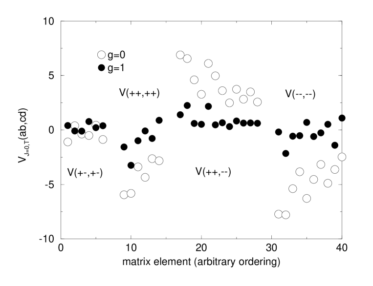
FIG. 1.: $J=0$ pairing matrix elements for realistic interaction in $sd$-$pf$ shell model calculations. $g=1$ corresponds to original, realistic Hamiltonian that has a ‘bad’ sign; $g=0$ is an interaction minimally deformed to have a ‘good’ sign. $x$-axis is arbitrary ordering of $J=0$ matrix elements. ‘$+$’ denotes the $sd$ shell while ‘-’ denotes the $pf$ shell.

REFERENCES

- [1] G. H. Lang, C. W. Johnson, S. E. Koonin, and W. E. Ormand, Phys. Rev. C 48, 1518 (1993).
- [2] Y. Alhassid, D. J. Dean, S. E. Koonin, G. Lang, and W. E. Ormand, Phys. Rev. Lett. 72, 613 (1994).
- [3] S. E. Koonin, D. J. Dean, and K. Langanke, Phys. Rep. 278,2 (1997).
- [4] E. Caurier, G. Martinez-Pinedo, F. Nowacki, A. Poves, J. Retamosa, and A. Zuker, Phys. Rev. C 59, 2033 (1999).
- [5] D.J. Dean, M.T. Ressell, M. Hjorth-Jensen, S.E. Koonin, K. Langanke, and A. Zuker, Phys. Rev. C 59, 2474 (1999); P.-G. Reinhard, D.J. Dean, W. Nazarewicz, J. Dobaczewski, J.A. Maruhn, and M.R. Strayer, Phys. Rev. C 60, 014316 (1999).
- [6] B. H. Wildenthal, Prog. Part. Nucl. Phys. 11, 5 (1984).
- [7] A. R. Edmonds, Angular Momentum in Quantum Mechanics, Princeton University Press (1960).