Chiral quark-soliton model in the Wigner-Seitz approximation

Abstract

In this paper we study the modification of the properties of the nucleon in the nucleus within the quark-soliton model. This is a covariant, dynamical model, which provides a non–linear representation of the spontaneously broken $SU(2)_{L}\times SU(2)_{R}$ symmetry of QCD. The effects of the nuclear medium are accounted for by using the Wigner-Seitz approximation and therefore reducing the complex many-body problem to a simpler single-particle problem. We find a minimum in the binding energy at finite density, a change in the isoscalar nucleon radius and a reduction of the in-medium pion decay constant. The latter is consistent with a partial restoration of chiral symmetry at finite density, which is predicted by other models.

I Introduction

In this paper we want to address the possibility that the nucleon properties be modified in the nuclear medium. In a conventional nuclear physics approach, where nucleons and mesons are elementary degrees of freedom, such question cannot be answered consistently and any modification of the nucleon properties has to be put in by hand. In order to address the problem, one has to consider models in which the substructure of the nucleon is not neglected (see, e.g, Refs. [1, 2, 3]), and properly implement these models in order to account for the presence of a medium.

In the present work we have considered a chiral model of the nucleon, which has been developed by Diakonov et al. [4, 5] on the basis of the instanton picture of the QCD vacuum. It provides a low-energy approximation to QCD that incorporates a non-linear representation of the spontaneously broken chiral symmetry. In this framework pions emerge as Goldstone bosons, dynamically generated by the Dirac sea. Vacuum fluctuations (quark loops) are described by an effective action that yields the pion kinetic term, — which is already included at the classical level in the Lagrangian of other chiral models, — and higher order non-local contributions. The model is also Lorentz covariant and has essentially only one free parameter (apart from the regularization scale), namely the constituent quark mass. Although the latter should in principle be momentum dependent, in practice a constant value is usually chosen, which better reproduces the phenomenological properties. The model has been successfully applied to the description of a variety of nucleon properties [4, 5, 6, 7].

Solving the many-body problem is already a formidable task in a conventional nuclear physics approach, the more so, of course, when one deals with extended objects. Early attempts treated nuclear matter as a crystal, letting the particles sit on a regular lattice [8, 9, 10, 11]. However, one has still to face serious computational difficulties in properly imposing the Bloch boundary conditions and moreover, nuclear matter does not show long-range crystalline order. These facts prompt the application of an approximation first introduced by Wigner and Seitz [12], in which the effect of the surrounding matter on each particle is accounted in an average manner, by enclosing it in a spherically symmetric cell: This technique does not depend on any particular structure of the lattice and it is particularly suitable for nuclear matter, which may be pictured more as a fluid than a crystal. In this way, a complex many-body problem is reduced to a single particle problem, where the effects of the nuclear medium enter only through average boundary conditions. The long-range order implied by imposing periodic boundary conditions gives rise to a band structure of the energy levels and one has to choose suitable boundary conditions for the lowest and highest energy levels.

The Wigner-Seitz approximation to the treatment of soliton matter has already been applied using other models of the nucleon structure: The Skyrme model [13, 14], non-topological soliton models [15, 16, 17], the hybrid soliton model [18, 19, 20, 17] and the global color model [21, 22, 23]. In these models the boundary conditions for the spherically symmetric bottom level of the band are an extension to a Dirac spinor of the non-relativistic requirement of having a flat wave function. Moreover, in the chiral soliton models [17, 18, 19, 20] the requirement of unit topological number inside the cell is also taken into account through the boundary condition on the chiral angle.

In this work we explore the sensitivity of the calculation to the choice of different boundary conditions, by also imposing the requirement of flatness on the chiral angle, as in Refs. [8, 14]. We also show that it does not make sense to discuss the band structure of the nuclear system without accounting for the spurious contribution to the energy stemming from the center-of-mass motion of the bags, since the corrections turn out to be larger than the band width and strongly dependent on the boundary condition for the level.

Another important difference of the present work from the above mentioned calculations is the fact that here we also account for contributions coming from the Dirac sea. Since the chiral field is a mean field, it means that we include one-loop quark fluctuations. The latter generate the kinetic pion term, — which is included by hand in the model Lagrangians of Refs. [17, 18, 19, 20], — and a (attractive) non-local contribution, which is known to be important for the calculation of free nucleon properties [4, 5, 6, 7]. Dirac fluctuations are usually neglected in the in-medium calculations, although there is no reason to expect they are negligible or at least independent of the density.

The paper is organized as follows: In Sections II A and II B we briefly discuss the main features of the quark-soliton model and the approximations employed in its implementation; in Sections II C–II H we introduce the Wigner-Seitz approximation, the appropriate boundary conditions for the fields and show how a few observables can be calculated in this model. A new orthonormal and complete basis in the elementary cell is also obtained, in which physical quantities, such as the vacuum energy, are expressed. In Section III we present the numerical results, obtained by solving the equations of motion. Finally, in Section IV we draw our conclusions and discuss possible future developments of the model.

II Nucleonic and nuclear models

A Chiral quark-soliton model

The chiral soliton model [4, 5, 6], which provides a non-linear representation of the $SU(2)_{L}\times SU(2)_{R}$ symmetry of QCD, is based on the lagrangian

$${\cal L} = \overline{\psi}\left[i\hbox to0.0pt{/\hss}\partial-MU_{5}(x)\right]\psi,$$ (1)

where $\psi$ represents the quark fields, carrying color, flavor and Dirac indices, while $U_{5}$ is a chiral field defined as

$$U_{5}(x) = \frac{1+\gamma_{5}}{2}\ U^{\dagger}(x)+\frac{1-\gamma_{5}}{2}\ U(x)$$ (2)

$$U(x) = \exp\left[i\mathchoice{{\hbox{\boldmath$\displaystyle\tau$}}}{{\hbox{\boldmath$\textstyle\tau$}}}{{\hbox{\boldmath$\scriptstyle\tau$}}}{{\hbox{\boldmath$\scriptscriptstyle\tau$}}}\cdot\mathchoice{{\hbox{\boldmath$\displaystyle\theta$}}}{{\hbox{\boldmath$\textstyle\theta$}}}{{\hbox{\boldmath$\scriptstyle\theta$}}}{{\hbox{\boldmath$\scriptscriptstyle\theta$}}}(x)\right].$$ (3)

The large ($\cong 350$ MeV) dynamical quark mass $M$ which appears in Eq. (1) is the result of the spontaneous breakdown of chiral symmetry, which also accounts for the appearance of massless Nambu-Goldstone pions. In this model the nucleon emerges as a bound state of $N_{c}$ quarks in a color singlet state, kept together by the chiral mean field. Note that no explicit kinetic energy term for the pion is present in (1): Actually, the $\psi$ and $U$ fields are not independent and the latter is in the end interpreted as a composite field in the quark-antiquark channel.

Introducing the familiar hedgehog shape of the soliton,

$$U(x) = \exp\left\{i\mathchoice{{\hbox{\boldmath$\displaystyle\tau$}}}{{\hbox{\boldmath$\textstyle\tau$}}}{{\hbox{\boldmath$\scriptstyle\tau$}}}{{\hbox{\boldmath$\scriptscriptstyle\tau$}}}\cdot\hat{\mathchoice{{\hbox{\boldmath$\displaystyle r$}}}{{\hbox{\boldmath$\textstyle r$}}}{{\hbox{\boldmath$\scriptstyle r$}}}{{\hbox{\boldmath$\scriptscriptstyle r$}}}}\ \theta(r)\right\},$$ (4)

the quark hamiltonian reads

$$H = -i\mathchoice{{\hbox{\boldmath$\displaystyle\alpha$}}}{{\hbox{\boldmath$\textstyle\alpha$}}}{{\hbox{\boldmath$\scriptstyle\alpha$}}}{{\hbox{\boldmath$\scriptscriptstyle\alpha$}}}\cdot\mathchoice{{\hbox{\boldmath$\displaystyle\nabla$}}}{{\hbox{\boldmath$\textstyle\nabla$}}}{{\hbox{\boldmath$\scriptstyle\nabla$}}}{{\hbox{\boldmath$\scriptscriptstyle\nabla$}}}+\beta M\left[\cos\theta(r)-i\gamma_{5}\mathchoice{{\hbox{\boldmath$\displaystyle\tau$}}}{{\hbox{\boldmath$\textstyle\tau$}}}{{\hbox{\boldmath$\scriptstyle\tau$}}}{{\hbox{\boldmath$\scriptscriptstyle\tau$}}}\cdot\hat{\mathchoice{{\hbox{\boldmath$\displaystyle r$}}}{{\hbox{\boldmath$\textstyle r$}}}{{\hbox{\boldmath$\scriptstyle r$}}}{{\hbox{\boldmath$\scriptscriptstyle r$}}}}\sin\theta(r)\right].$$ (5)

However, solutions to the classical field equations derived from (5) do not describe nucleon and $\Delta$ states, since angular momentum and isospin do not commute with $H$: One defines the so called grand spin, $\mathchoice{{\hbox{\boldmath$\displaystyle K$}}}{{\hbox{\boldmath$\textstyle K$}}}{{\hbox{\boldmath$\scriptstyle K$}}}{{\hbox{\boldmath$\scriptscriptstyle K$}}}=\mathchoice{{\hbox{\boldmath$\displaystyle J$}}}{{\hbox{\boldmath$\textstyle J$}}}{{\hbox{\boldmath$\scriptstyle J$}}}{{\hbox{\boldmath$\scriptscriptstyle J$}}}+\mathchoice{{\hbox{\boldmath$\displaystyle\tau$}}}{{\hbox{\boldmath$\textstyle\tau$}}}{{\hbox{\boldmath$\scriptstyle\tau$}}}{{\hbox{\boldmath$\scriptscriptstyle\tau$}}}/2$, for which $\left[H,\mathchoice{{\hbox{\boldmath$\displaystyle K$}}}{{\hbox{\boldmath$\textstyle K$}}}{{\hbox{\boldmath$\scriptstyle K$}}}{{\hbox{\boldmath$\scriptscriptstyle K$}}}\right]=0$, and the quark wave function can be written as

$$\psi = \frac{1}{\sqrt{4\pi}}\left(\begin{array}[]{c}u(r)\ \xi\\ v(r)\ i\mathchoice{{\hbox{\boldmath$\displaystyle\sigma$}}}{{\hbox{\boldmath$\textstyle\sigma$}}}{{\hbox{\boldmath$\scriptstyle\sigma$}}}{{\hbox{\boldmath$\scriptscriptstyle\sigma$}}}\cdot\hat{\mathchoice{{\hbox{\boldmath$\displaystyle r$}}}{{\hbox{\boldmath$\textstyle r$}}}{{\hbox{\boldmath$\scriptstyle r$}}}{{\hbox{\boldmath$\scriptscriptstyle r$}}}}\ \xi\end{array}\right),$$ (8)

where $\xi$ is the grand spin state fulfilling

$$\left(\mathchoice{{\hbox{\boldmath$\displaystyle\sigma$}}}{{\hbox{\boldmath$\textstyle\sigma$}}}{{\hbox{\boldmath$\scriptstyle\sigma$}}}{{\hbox{\boldmath$\scriptscriptstyle\sigma$}}}+\mathchoice{{\hbox{\boldmath$\displaystyle\tau$}}}{{\hbox{\boldmath$\textstyle\tau$}}}{{\hbox{\boldmath$\scriptstyle\tau$}}}{{\hbox{\boldmath$\scriptscriptstyle\tau$}}}\right)\ \xi=0$$ (9)

and the normalization is

$$4\pi\int_{0}^{\infty}dr\ r^{2}\ \overline{\psi}\gamma^{0}\psi=1.$$ (10)

Good spin and isospin quantum numbers may be obtained in the end in a semiclassical approximation by quantizing the adiabatic rotational motion in isospin space [24, 2]. However, in the present paper, for the sake of simplicity, we limit ourselves to consider soliton matter, leaving the projection of spin-isospin quantum numbers for future work.

The classical solutions are found self-consistently by solving the equations obtained by minimization of the total energy

$$E_{\text{tot}}[\psi,\overline{\psi},\theta] = N_{c}E_{\text{val}}[\psi,\overline{\psi},\theta]+E_{\text{vac}}[\theta],$$ (11)

where $E_{\text{val}}\equiv\langle\psi|H|\psi\rangle$ and $E_{\text{vac}}$ are the valence and vacuum part of the energy, respectively. The vacuum energy $E_{\text{vac}}$ incorporates, at the mean field level, one-quark-loop contributions and, formally, can be evaluated through the effective action, which is obtained by considering the following path integral over the quark fields

$$\exp\left\{iS_{\text{eff}}[U]\right\} = \int[d\overline{\psi}][d\psi]\ \exp\left\{i\int d^{4}x\ {\overline{\psi}(x)\left[i\hbox to0.0pt{/\hss}\partial-MU_{5}(x)\right]\psi(x)}\right\}$$ (12)

$$= \left[\det\left(i\hbox to0.0pt{/\hss}\partial-MU_{5}(x)\right)\right]^{N_{c}}.$$ (13)

The latter can be easily cast in a more suitable form by means of simple algebraic manipulations

$$S_{\text{eff}}[U] = -\frac{i}{2}N_{c}\,\text{tr}\,\log\left[\frac{\Box+M^{2}+iM\hbox to0.0pt{/\hss}\partial U_{5}(x)}{\Box+M^{2}}\right],$$ (14)

where the trace is over Dirac and flavor indices. Despite its apparent simplicity, (14) is actually a complicate nonlocal object.

Although a local derivative expansion of course is possible, it is of little practical use in this case, since the soliton field turns out to vary significantly over the relevant distance scale $M^{-1}$ and no stable solutions are found for expansions up to sixth order in derivatives [25]. Kahana and Ripka [33] on the other hand have developed a numerical algorithm to directly evaluate vacuum polarization contributions to soliton observables. This technique has been extended in Ref. [6] to the calculation of nucleon observables, that is after collective quantization has been applied to project out states of definite spin and isospin.

B Effective action up to second order in the soliton field

Another path, to which we shall adhere in the following, has been followed in Refs. [4, 27] by expanding (14) up to second order in $M(\hbox to0.0pt{/\hss}\partial U_{5})$, obtaining

$$S^{(2)}_{\text{eff}}[U] \approx \frac{i}{4}N_{c}\,\text{tr}\,\langle x|\frac{1}{\Box+M^{2}}\left[iM\hbox to0.0pt{/\hss}\partial U_{5}\right]\frac{1}{\Box+M^{2}}\left[iM\hbox to0.0pt{/\hss}\partial U_{5}\right]|x\rangle$$ (15)

$$= -\frac{1}{4}N_{c}\,\text{tr}\,\int d^{4}xd^{4}x^{\prime}V(x)K(x,x^{\prime})V(x^{\prime}),$$ (16)

where

$$V(x) = iM\hbox to0.0pt{/\hss}\partial U_{5}$$ (17)

$$K(x,x^{\prime}) = -iG(x,x^{\prime})G(x^{\prime},x)$$ (18)

$$(\Box+M^{2})G(x,x^{\prime}) = \delta^{4}(x-x^{\prime}).$$ (19)

Note that in the standard derivative expansion the second order action would read

$$S^{(2)}_{\text{eff}}[U] \approx -\frac{i}{4}N_{c}M^{2}\,\text{tr}\,\left[\hbox to0.0pt{/\hss}\partial U_{5}\hbox to0.0pt{/\hss}\partial U_{5}\right]\langle x|\frac{1}{\Box+M^{2}}\frac{1}{\Box+M^{2}}|x\rangle.$$ (20)

In contrast to (20) , Eq. (16) does not assume a slowly varying soliton field and gives rise to non-local contributions. Furthermore, one can see that it gives a good approximation both for small and large momenta, thus providing an interpolation formula between these regimes [4, 5].

Specializing to static field configurations, introducing $E^{(2)}_{\text{vac}}\equiv-S^{(2)}_{\text{eff}}/\int dx^{0}$ and going to momentum space, one gets

$$E^{(2)}_{\text{vac}}=\frac{N_{c}}{4}\int\frac{d\mathchoice{{\hbox{\boldmath$\displaystyle q$}}}{{\hbox{\boldmath$\textstyle q$}}}{{\hbox{\boldmath$\scriptstyle q$}}}{{\hbox{\boldmath$\scriptscriptstyle q$}}}}{(2\pi)^{3}}\text{tr}[V(\mathchoice{{\hbox{\boldmath$\displaystyle q$}}}{{\hbox{\boldmath$\textstyle q$}}}{{\hbox{\boldmath$\scriptstyle q$}}}{{\hbox{\boldmath$\scriptscriptstyle q$}}})V(-\mathchoice{{\hbox{\boldmath$\displaystyle q$}}}{{\hbox{\boldmath$\textstyle q$}}}{{\hbox{\boldmath$\scriptstyle q$}}}{{\hbox{\boldmath$\scriptscriptstyle q$}}})]K(q),$$ (21)

where

$$\text{tr}[V(\mathchoice{{\hbox{\boldmath$\displaystyle q$}}}{{\hbox{\boldmath$\textstyle q$}}}{{\hbox{\boldmath$\scriptstyle q$}}}{{\hbox{\boldmath$\scriptscriptstyle q$}}})V(-\mathchoice{{\hbox{\boldmath$\displaystyle q$}}}{{\hbox{\boldmath$\textstyle q$}}}{{\hbox{\boldmath$\scriptstyle q$}}}{{\hbox{\boldmath$\scriptscriptstyle q$}}})]=\frac{8M^{2}}{f_{\pi}^{2}}q^{2}[\phi_{0}(q)\phi_{0}(q)+\phi_{i}(\mathchoice{{\hbox{\boldmath$\displaystyle q$}}}{{\hbox{\boldmath$\textstyle q$}}}{{\hbox{\boldmath$\scriptstyle q$}}}{{\hbox{\boldmath$\scriptscriptstyle q$}}})\phi_{i}(-\mathchoice{{\hbox{\boldmath$\displaystyle q$}}}{{\hbox{\boldmath$\textstyle q$}}}{{\hbox{\boldmath$\scriptstyle q$}}}{{\hbox{\boldmath$\scriptscriptstyle q$}}})],$$ (22)

with

$$\phi_{0}(q) = 4\pi f_{\pi}\int_{0}^{\infty}dr\,r^{2}j_{0}(qr)[\cos\theta(r)-1]$$ (24)

$$\phi_{i}(\mathchoice{{\hbox{\boldmath$\displaystyle q$}}}{{\hbox{\boldmath$\textstyle q$}}}{{\hbox{\boldmath$\scriptstyle q$}}}{{\hbox{\boldmath$\scriptscriptstyle q$}}}) = i\hat{\mathchoice{{\hbox{\boldmath$\displaystyle q$}}}{{\hbox{\boldmath$\textstyle q$}}}{{\hbox{\boldmath$\scriptstyle q$}}}{{\hbox{\boldmath$\scriptscriptstyle q$}}}}_{i}4\pi f_{\pi}\int_{0}^{\infty}dr\,r^{2}j_{1}(qr)\sin\theta(r)\equiv i\hat{\mathchoice{{\hbox{\boldmath$\displaystyle q$}}}{{\hbox{\boldmath$\textstyle q$}}}{{\hbox{\boldmath$\scriptstyle q$}}}{{\hbox{\boldmath$\scriptscriptstyle q$}}}}_{i}\phi(q),$$ (25)

and

$$K(q) = \int d\mathchoice{{\hbox{\boldmath$\displaystyle r$}}}{{\hbox{\boldmath$\textstyle r$}}}{{\hbox{\boldmath$\scriptstyle r$}}}{{\hbox{\boldmath$\scriptscriptstyle r$}}}\,\text{e}^{i\mathchoice{{\hbox{\boldmath$\displaystyle q$}}}{{\hbox{\boldmath$\textstyle q$}}}{{\hbox{\boldmath$\scriptstyle q$}}}{{\hbox{\boldmath$\scriptscriptstyle q$}}}\cdot\mathchoice{{\hbox{\boldmath$\displaystyle r$}}}{{\hbox{\boldmath$\textstyle r$}}}{{\hbox{\boldmath$\scriptstyle r$}}}{{\hbox{\boldmath$\scriptscriptstyle r$}}}}K(r)$$ (26)

$$K(r) = \frac{1}{8\pi^{5}}\int_{0}^{\infty}dk\,k^{2}\int_{0}^{\infty}dk^{\prime}\,{k^{\prime}}^{2}\frac{\pi}{E_{k}E_{k^{\prime}}}\frac{C\left[\left(k+k^{\prime}\right)/2\right]}{E_{k}+E_{k^{\prime}}}j_{0}(kr)j_{0}(k^{\prime}r).$$ (28)

In (LABEL:eq:Kqr) $E_{k}=\sqrt{k^{2}+M^{2}}$, whereas $C(k)$ is a regulating function, which will be discussed later.

Although here and in the following we display, for convenience, formulae using a momentum cut-off regularization scheme, we shall employ also the Pauli-Villars regularization, also to be discussed later.

$E^{(2)}_{\text{vac}}$ must contain the meson kinetic energy contribution, which can be seen [27] to correspond to keeping only the $q=0$ term in an expansion of $K(q)$ in (21). This requirement fixes the normalization of $K$ in such a way that

$$K(0)\equiv\frac{1}{8\pi^{2}}\int_{0}^{\infty}dk\,k^{2}\frac{C(k)}{E_{k}^{3}}=\frac{f_{\pi}^{2}}{4N_{c}M^{2}}.$$ (29)

Then one finds $E^{(2)}_{\text{vac}}=E^{\text{kin}}+\widetilde{E}^{(2)}$, where

$$E^{\text{kin}} = \frac{1}{4\pi^{2}}\int_{0}^{\infty}dq\,q^{4}[\phi_{0}^{2}(q)+\phi^{2}(q)]$$ (30)

$$= 2\pi f_{\pi}^{2}\int_{0}^{\infty}dr[r^{2}{\theta^{\prime}}^{2}+2\sin^{2}\theta],$$ (31)

with $\theta^{\prime}=d\theta/dr$, and

$$\widetilde{E}^{(2)}=\frac{1}{4\pi^{2}}\int_{0}^{\infty}dq\,q^{4}\left[\frac{K(q)}{K(0)}-1\right][\phi_{0}^{2}(q)+\phi^{2}(q)].$$ (32)

The propagator $K(q)$ can be brought (see Appendix A) into the form

$$K(q)=\frac{1}{8\pi^{2}q}\int_{0}^{\infty}dk\frac{k}{E_{k}}\int_{|k-q|}^{k+q}dk^{\prime}\frac{k^{\prime}}{E_{k^{\prime}}}\frac{C\left[\left(k+k^{\prime}\right)/2\right]}{E_{k}+E_{k^{\prime}}}.$$ (33)

C Nuclear matter in the Wigner-Seitz approximation

In order to describe nuclear matter we shall employ, as anticipated in the Introduction, the Wigner-Seitz (WS) approximation [12], which amounts to enclose the fields in a spherically symmetric cell of radius R, imposing suitable boundary conditions. Before discussing our choice of boundary conditions, let us describe the evaluation of the vacuum energy in the WS cell.

We have first to find an orthonormal and complete basis of functions inside the elementary cell. We have chosen a spherical basis, in which the radial dependence is expressed through spherical Bessel functions, which have vanishing derivative at the boundary. This is the most useful basis in which to perform the calculation, when flat (zero derivative) boundary conditions for the fields are invoked. More details on the basis are given in the Appendix B. All the quantities involved in the calculation of the vacuum energy turn out to converge quickly using this basis. They also converge rapidly when zero boundary conditions are employed for the fields.

Starting again from the static limit of (16) and (18), one can introduce the Bessel transform of $K(\mathchoice{{\hbox{\boldmath$\displaystyle r$}}}{{\hbox{\boldmath$\textstyle r$}}}{{\hbox{\boldmath$\scriptstyle r$}}}{{\hbox{\boldmath$\scriptscriptstyle r$}}},\mathchoice{{\hbox{\boldmath$\displaystyle r$}}}{{\hbox{\boldmath$\textstyle r$}}}{{\hbox{\boldmath$\scriptstyle r$}}}{{\hbox{\boldmath$\scriptscriptstyle r$}}}^{\prime})$ as

$$K(\mathchoice{{\hbox{\boldmath$\displaystyle r$}}}{{\hbox{\boldmath$\textstyle r$}}}{{\hbox{\boldmath$\scriptstyle r$}}}{{\hbox{\boldmath$\scriptscriptstyle r$}}},\mathchoice{{\hbox{\boldmath$\displaystyle r$}}}{{\hbox{\boldmath$\textstyle r$}}}{{\hbox{\boldmath$\scriptstyle r$}}}{{\hbox{\boldmath$\scriptscriptstyle r$}}}^{\prime})=\sum_{lm}\sum_{\alpha_{l}\alpha^{\prime}_{l}}Y_{lm}(\hat{\mathchoice{{\hbox{\boldmath$\displaystyle r$}}}{{\hbox{\boldmath$\textstyle r$}}}{{\hbox{\boldmath$\scriptstyle r$}}}{{\hbox{\boldmath$\scriptscriptstyle r$}}}})Y^{*}_{lm}(\hat{\mathchoice{{\hbox{\boldmath$\displaystyle r$}}}{{\hbox{\boldmath$\textstyle r$}}}{{\hbox{\boldmath$\scriptstyle r$}}}{{\hbox{\boldmath$\scriptscriptstyle r$}}}}^{\prime})\rho_{\alpha_{l}}(r)\rho_{\alpha^{\prime}_{l}}(r^{\prime})K_{l}(\alpha_{l},\alpha^{\prime}_{l}),$$ (34)

where

$$\rho_{\alpha_{l}}(r)\equiv\kappa_{\alpha_{l}}j_{l}({\alpha_{l}}r/R),\quad\frac{d\rho_{\alpha_{l}}}{dr}\Big{|}_{r=R}=0,$$ (35)

$\kappa_{\alpha_{l}}$ being a normalization constant. Inserting (34) into (16), one finds

$$E^{(2)}_{\text{WS}}=E^{\text{kin}}_{\text{WS}}+\widetilde{E}^{(2)}_{\text{WS}},$$ (36)

where, as in the previous subsection, the kinetic energy contribution, — the one stemming from the local part of $K(\mathchoice{{\hbox{\boldmath$\displaystyle r$}}}{{\hbox{\boldmath$\textstyle r$}}}{{\hbox{\boldmath$\scriptstyle r$}}}{{\hbox{\boldmath$\scriptscriptstyle r$}}},\mathchoice{{\hbox{\boldmath$\displaystyle r$}}}{{\hbox{\boldmath$\textstyle r$}}}{{\hbox{\boldmath$\scriptstyle r$}}}{{\hbox{\boldmath$\scriptscriptstyle r$}}}^{\prime})=\delta(\mathchoice{{\hbox{\boldmath$\displaystyle r$}}}{{\hbox{\boldmath$\textstyle r$}}}{{\hbox{\boldmath$\scriptstyle r$}}}{{\hbox{\boldmath$\scriptscriptstyle r$}}}-\mathchoice{{\hbox{\boldmath$\displaystyle r$}}}{{\hbox{\boldmath$\textstyle r$}}}{{\hbox{\boldmath$\scriptstyle r$}}}{{\hbox{\boldmath$\scriptscriptstyle r$}}}^{\prime})K_{0}(r)+...$, — has been separated. Indeed, one has

$$E^{\text{kin}}_{\text{WS}}=8\pi N_{c}M^{2}\int_{0}^{R}drK_{0}(r)[r^{2}{\theta^{\prime}}^{2}(r)+2\sin^{2}\theta(r)],$$ (37)

with

$$K_{0}(r)=\sum_{l}\sum_{\alpha_{l}}\frac{2l+1}{16\pi}\frac{C(\alpha_{l}/R)}{E^{3}_{\alpha_{l}/R}}\rho^{2}_{\alpha_{l}}(r)$$ (38)

and $E_{\alpha_{l}/R}=\sqrt{(\alpha_{l}/R)^{2}+M^{2}}$.

In the limit $R\to\infty$ one can check that

$$K_{0}(r)\to\frac{1}{8\pi^{2}}\int_{0}^{\infty}dk\,k^{2}\frac{C(k)}{E_{k}^{3}}\equiv\frac{f_{\pi}^{2}}{4N_{c}M^{2}}.$$ (39)

As in the free space case, this fixes the normalization of $K_{0}(r)$ in such a way that

$$K_{0}(0)=\frac{1}{16\pi}\sum_{\alpha_{0}}\frac{C(\alpha_{0}/R)}{E^{3}_{\alpha_{0}/R}}\rho^{2}_{\alpha_{0}}(r)=\frac{f_{\pi}^{2}}{4N_{c}M^{2}}.$$ (40)

Then, one can write

$$E^{\text{kin}}_{\text{WS}}=2\pi f_{\pi}^{2}\int_{0}^{R}dr\frac{K_{0}(r)}{K_{0}(0)}[r^{2}{\theta^{\prime}}^{2}(r)+2\sin^{2}\theta(r)].$$ (41)

As we shall discuss below, one can view

$$f_{\pi,\text{WS}}^{2}\equiv f_{\pi}^{2}\frac{K_{0}(r)}{K_{0}(0)}$$ (42)

as an in-medium, $r$-dependent pion decay “constant”.

On the other hand, the non-local contribution $\widetilde{E}^{(2)}_{\text{WS}}$, — the in-medium extension of (32), — can be cast into the following form:

$$\widetilde{E}^{(2)}_{\text{WS}} = \frac{8\pi N_{c}M}{f_{\pi}^{2}}\sum_{\alpha\alpha^{\prime}}\big{\{}\frac{1}{3}f_{0}(\alpha_{0})\Delta K_{0}(\alpha_{0},\alpha^{\prime}_{0})f_{0}(\alpha^{\prime}_{0})+f_{1}(\alpha_{1})\Delta K_{1}(\alpha_{1},\alpha^{\prime}_{1})f_{1}(\alpha^{\prime}_{1})$$ (44)

$$\qquad\qquad\qquad+\frac{2}{3}f_{2}(\alpha_{2})\Delta K_{2}(\alpha_{2},\alpha^{\prime}_{2})f_{2}(\alpha^{\prime}_{2})\big{\}},$$

where

$$f_{0}(\alpha_{0}) = M^{1/2}\int_{0}^{R}dr\,r^{2}\rho_{\alpha_{0}}(r)\left[\cos\theta(r)\theta^{\prime}(r)+2\frac{\sin\theta(r)}{r}\right]$$ (46)

$$f_{1}(\alpha_{1}) = M^{1/2}\int_{0}^{R}dr\,r^{2}\rho_{\alpha_{1}}(r)\sin\theta(r)\theta^{\prime}(r)$$ (47)

$$f_{2}(\alpha_{2}) = M^{1/2}\int_{0}^{R}dr\,r^{2}\rho_{\alpha_{2}}(r)\left[\cos\theta(r)\theta^{\prime}(r)-\frac{\sin\theta(r)}{r}\right]$$ (48)

and

$$\Delta K_{l}(\alpha_{l},\alpha^{\prime}_{l}) = \frac{1}{8\pi^{2}}\sum_{LL^{\prime}}(2L+1)(2L^{\prime}+1)\left(\begin{array}[]{ccc}L&L^{\prime}&l\\ 0&0&0\end{array}\right)^{2}\kappa_{lLL^{\prime}}(\alpha_{l},\alpha^{\prime}_{l})$$ (52)

$$\kappa_{lLL^{\prime}}(\alpha_{l},\alpha^{\prime}_{l}) = \sum_{\alpha_{L}\alpha_{L^{\prime}}}\frac{\pi}{E_{\alpha_{L}}}\left[\frac{C\left[\left(\alpha_{L}+\alpha_{L^{\prime}}\right)/2\right]}{E_{\alpha_{L^{\prime}}}(E_{\alpha_{L}}+E_{\alpha_{L^{\prime}}})}-\frac{C(\alpha_{L})}{2E^{2}_{\alpha_{L}}}\right]\xi(\alpha_{l},\alpha_{L},\alpha_{L^{\prime}})\xi(\alpha^{\prime}_{l},\alpha_{L},\alpha_{L^{\prime}})$$ (53)

$$\xi(\alpha_{l},\alpha_{L},\alpha_{L^{\prime}}) = \int_{0}^{R}dr\,r^{2}\rho_{\alpha_{l}}(r)\rho_{\alpha_{L}}(r)\rho_{\alpha_{L^{\prime}}}(r).$$ (54)

One should now notice that the straightforward application of (14) to the Wigner-Seitz cell is incomplete, because it does not account for the Casimir energy intrinsically connected with the change of topology, which is present even in the absence of background fields. As a matter of fact one should write:

$$S_{\text{eff}}[U] = -\frac{i}{2}N_{c}\,\text{tr}\,\left\{\log\left[\Box+M^{2}+iM\hbox to0.0pt{/\hss}\partial U_{5}(x)\right]_{\text{WS}}-\log\left[\Box+M^{2}\right]_{\text{free}}\right\}$$ (55)

$$\equiv -\frac{i}{2}N_{c}\,\text{tr}\,\log\left[\frac{\Box+M^{2}+iM\hbox to0.0pt{/\hss}\partial U_{5}(x)}{\Box+M^{2}}\right]_{\text{WS}}+\Delta S_{\text{eff}}^{\text{Casimir}},$$ (56)

where

$$\Delta S_{\text{eff}}^{\text{Casimir}} \equiv -\frac{i}{2}N_{c}\,\text{tr}\,\left\{\log\left[\Box+M^{2}\right]_{\text{WS}}-\log\left[\Box+M^{2}\right]_{\text{free}}\right\}.$$ (57)

Note that the first term in (55) is just the application of Eq. (14) to the Wigner-Seitz case; on the other hand, the second term is the genuine Casimir energy due to the change of configuration space. By performing the intermediate algebra one obtains

$$\Delta S_{\text{eff}}^{\text{Casimir}} \equiv 4N_{c}T\left\{\sum_{l}\sum_{\alpha_{l}}(2l+1)\sqrt{M^{2}+\frac{\alpha_{l}^{2}}{R^{2}}}-\lim_{R\rightarrow\infty}\sum_{l}\sum_{\alpha_{l}}(2l+1)\sqrt{M^{2}+\frac{\alpha_{l}^{2}}{R^{2}}}\right\}.$$ (58)

The Casimir energy, which is obtained by dividing this expression by the time $-T$, has now the expected form: It is the difference between the zero-point energy in the finite volume, obtained by filling all the negative energy orbitals in the Dirac sea, and the same expression in free space. As it stands, however, Eq. (58) is badly divergent and needs to be regularized. Such a task has been recently carried out for massive fermions, in the context of the MIT bag model, in Ref. [28] by means of the zeta function regularization technique. In the present work we will neglect this contribution to the total energy.

D Regularization of integrals and sums

In calculating the vacuum contributions to the physical observables one has to deal with the appearance of divergent expressions. In this paper we consider two different regularization schemes, applying a momentum cutoff and using the Pauli-Villars regularization.

In the first case we introduce a regulating function, which suppresses the contribution to integrals and sums at momenta $k\gg\Lambda$, where the scale $\Lambda$ is determined by fitting the pion decay constant in free space (see Eq. (29). The regulating function we have chosen has the form

$$C(k)=\frac{1+1/e}{\exp\left[\left(k^{2}-\Lambda^{2}\right)/\Lambda^{2}\right]+1}.$$ (59)

In the Pauli-Villars regulating scheme [29], on the other hand, the divergent contributions are eliminated through the subtraction

$$K(x,x^{\prime})\rightarrow K(x,x^{\prime})-K^{\text{PV}}(x,x^{\prime}),$$ (60)

where $K(x,x^{\prime})$ is the propagator previously defined, while in $K^{\text{PV}}(x,x^{\prime})$ the quark mass $M$ has been substituted by the mass scale $M_{\text{PV}}$, obtained again by fitting the free space pion decay constant:

$$M_{\text{PV}}=M\exp\left(\frac{2\pi^{2}f_{\pi}^{2}}{N_{c}M^{2}}\right).$$ (61)

E Pion decay constant

Let’s now consider the axial current. Its valence part is

$$A_{a}^{\mu}(x)=\overline{\psi}(x)\frac{\tau^{a}}{2}\gamma^{\mu}\gamma_{5}\psi(x).$$ (62)

We wish to calculate also the vacuum (i.e. from the Dirac sea at the one-quark-loop level) contribution to the axial current: This can be done by defining the generating functional

$$W[a]=\int\left[d\overline{\psi}d\psi\right]\exp\left\{i\int d^{4}x\left[\overline{\psi}\ \left(i\hbox to0.0pt{/\hss}\partial-MU_{5}\right)\psi-a_{\mu}^{a}A_{a}^{\mu}\right]\right\},$$ (63)

where $a_{a}^{\mu}$ are classical axial sources coupled to the quantum axial current; then, the vacuum axial current can be obtained by means of a functional derivative with respect to the source as

$$A_{a,\text{vac}}^{\mu}(x)=i\frac{\delta}{\delta a_{\mu}^{a}(x)}\ln W[a]\Bigg{|}_{a^{a}_{\mu}=0}.$$ (64)

Calculation provides

$$A_{a,\text{vac}}^{\mu}(x)=\frac{4N_{c}M^{2}}{f_{\pi}^{2}}\int d^{4}x^{\prime}K(x,x^{\prime})\left[\partial^{\mu}\phi_{0}(x^{\prime})\phi^{a}(x)-\partial^{\mu}\phi^{a}(x^{\prime})\phi_{0}(x)\right].$$ (65)

By setting

$$K(x,x^{\prime})=K_{0}(r)\delta^{4}(x-x^{\prime})+\Delta K(x,x^{\prime}),$$ (66)

where $K_{0}(r)$ is given by Eq. (38), one is able to write

$$A_{a}^{\mu}(x) = \overline{\psi}(x)\frac{\tau^{a}}{2}\gamma^{\mu}\gamma_{5}\psi(x)+\frac{4N_{c}M^{2}}{f_{\pi}^{2}}K_{0}(r)\left[\partial^{\mu}\phi_{0}(x)\phi^{a}(x)-\partial^{\mu}\phi^{a}(x)\phi_{0}(x)\right]$$ (68)

$$\quad+\frac{4N_{c}M^{2}}{f_{\pi}^{2}}\int d^{4}x^{\prime}\Delta K(x,x^{\prime})\left[\partial^{\mu}\phi_{0}(x^{\prime})\phi^{a}(x)-\partial^{\mu}\phi^{a}(x^{\prime})\phi_{0}(x)\right],$$

in which local and non-local contributions have been separated.

Remembering now that the pion decay constant is defined as

$$\langle 0|A_{a}^{\mu}(x)|\pi^{b}(p)\rangle=-ip^{\mu}f_{\pi}\delta_{a,b}e^{-ip\cdot x},$$ (69)

one is able to obtain the in-medium pion decay constant as

$$f_{\pi,\text{WS}}^{2}(r)=4N_{c}M^{2}K_{0}(r),$$ (70)

that is expression (42), which depends, in a medium, on the radial coordinate.

An estimate of the average value of $f_{\pi}$ at fixed density can be obtained by calculating the constant value of $f_{\pi,\text{WS}}$ that would yield the same pion kinetic energy as the $r$-dependent one (compare Eqs.  (31) and  (41)):

$$\langle f_{\pi}\rangle^{2}=\frac{\int_{0}^{R}dr\,f_{\pi,\text{WS}}^{2}(r)\left[r^{2}{\theta^{\prime}}^{2}(r)+\sin^{2}\theta(r)\right]}{\int_{0}^{R}dr\left[r^{2}{\theta^{\prime}}^{2}(r)+\sin^{2}\theta(r)\right]}.$$ (71)

F Axial coupling constant

The axial coupling constant, for a system with a finite pion mass is given by

$$\frac{1}{2}g_{A}=\langle p\uparrow|\int d\mathchoice{{\hbox{\boldmath$\displaystyle r$}}}{{\hbox{\boldmath$\textstyle r$}}}{{\hbox{\boldmath$\scriptstyle r$}}}{{\hbox{\boldmath$\scriptscriptstyle r$}}}A_{3}^{z}|p\uparrow\rangle.$$ (72)

The matrix element between proton states requires one to adopt a collective quantization procedure in order to project out the correct quantum numbers. In the case of $g_{A}$, — as discussed, e. g., in Ref. [30], — it amounts simply to multiply the expression for the hedgehog axial current by the matrix element of the cranking operator, $-1/3$. Furthermore, as discussed in Ref. [24], the $m_{\pi}=0$ limit requires one to perform first the angular integral and then the radial integral in (72), multiplying the result by a factor $3/2$.

Use of Eq. (68) yields

$$g_{A}=\int_{0}^{R}dr\,r^{2}\left[\frac{N_{c}}{2}(u^{2}-\frac{1}{3}v^{2})-\frac{4\pi}{3}f_{\pi,\text{WS}}^{2}\left(\theta^{\prime}+\frac{\sin(2\theta)}{r}\right)\right]-\int d\mathchoice{{\hbox{\boldmath$\displaystyle r$}}}{{\hbox{\boldmath$\textstyle r$}}}{{\hbox{\boldmath$\scriptstyle r$}}}{{\hbox{\boldmath$\scriptscriptstyle r$}}}\Delta A_{3}^{z},$$ (73)

with

$$\int d\mathchoice{{\hbox{\boldmath$\displaystyle r$}}}{{\hbox{\boldmath$\textstyle r$}}}{{\hbox{\boldmath$\scriptstyle r$}}}{{\hbox{\boldmath$\scriptscriptstyle r$}}}\Delta A_{3}^{z} = -\frac{16\pi N_{c}M^{2}}{3}\sum_{\alpha,\alpha^{\prime}}\left\{\overline{f}_{0}(\alpha_{0})\Delta K_{0}(\alpha_{0},\alpha^{\prime}_{0})f_{0}(\alpha^{\prime}_{0})+\overline{f}_{1}(\alpha_{1})\Delta K_{1}(\alpha_{1},\alpha^{\prime}_{1})f_{1}(\alpha^{\prime}_{1})\right\}$$ (74)

and

$$\overline{f}_{0}(\alpha_{0}) \equiv M^{3/2}\int_{0}^{R}dr\ r^{2}\ \rho_{\alpha_{0}}(r)\left(\cos\theta(r)-1\right)$$ (75)

$$\overline{f}_{1}(\alpha_{1}) \equiv M^{3/2}\int_{0}^{R}dr\ r^{2}\ \rho_{\alpha_{1}}(r)\sin\theta(r).$$ (76)

These are the expressions we shall employ in the next Section to evaluate the in-medium modification of the axial coupling constant.

G Equations of motion

The equations of motion are found by minimizing the total energy (11) with respect to the Dirac fields, $u$ and $v$, and to the chiral angle, $\theta$. It is convenient to write them in a dimensionless form by letting $q\to Mq$ and introducing

$$x=Mr,\quad\tilde{u}(x)=M^{-3/2}u(r),\quad\tilde{v}(x)=M^{-3/2}v(r).$$ (77)

Minimization of $\epsilon_{\text{tot}}\equiv E_{\text{tot}}/M=\epsilon_{\text{val}}+\epsilon^{(2)}_{\text{vac}}$ then yields

$$\frac{d\tilde{u}}{dx} = -\sin\theta\,\tilde{u}-(\epsilon_{\text{val}}+\cos\theta)\tilde{v}$$ (79)

$$\frac{d\tilde{v}}{dx} = -\left(\frac{2}{x}-\sin\theta\right)\tilde{v}+(\epsilon_{\text{val}}-\cos\theta)\tilde{u}$$ (80)

$$\frac{d^{2}\theta}{dx^{2}} + \frac{2}{x}\frac{d\theta}{dx}-\frac{\sin 2\theta}{x^{2}}+\frac{N_{c}M^{2}}{4\pi f_{\pi}^{2}}[(\tilde{u}^{2}-\tilde{v}^{2})\sin\theta+2\tilde{u}\tilde{v}\cos\theta]$$ (81)

$$+ \frac{2}{\pi}\sin\theta\int_{0}^{\infty}dq\,q^{2}\left[\frac{K(q)}{K(0)}-1\right]j_{0}(qx){\cal C}(q)$$ (82)

$$- \frac{2}{\pi}\cos\theta\int_{0}^{\infty}dq\,q^{2}\left[\frac{K(q)}{K(0)}-1\right]j_{1}(qx){\cal S}(q)=0,$$ (83)

where

$${\cal C}(q) = \int_{0}^{\infty}dx(qx)^{2}j_{0}(qx)[\cos\theta(x)-1]$$ (85)

$${\cal S}(q) = \int_{0}^{\infty}dx(qx)^{2}j_{1}(qx)\sin\theta(x),$$ (86)

and $K(q)$ is still given by (33), but now $k$, $k^{\prime}$ are dimensionless and $E_{k}\to\tilde{E}_{k}=\sqrt{k^{2}+1}$. This is a set of integro-differential equations that has to be solved iteratively as shown, for instance, in Ref. [27].

The same procedure, applied to the system enclosed into the WS cell, yields

$$\frac{d\tilde{u}}{dx} = -\sin\theta\,\tilde{u}-(\epsilon_{\text{val}}+\cos\theta)\tilde{v}$$ (88)

$$\frac{d\tilde{v}}{dx} = -\left(\frac{2}{x}-\sin\theta\right)\tilde{v}+(\epsilon_{\text{val}}-\cos\theta)\tilde{u}$$ (89)

$$\frac{d^{2}\theta}{dx^{2}} + 2\left[\frac{1}{x}+\frac{d}{dx}\ln K_{0}(x)\right]\frac{d\theta}{dx}-\frac{\sin 2\theta}{x^{2}}+\frac{1}{16\pi K_{0}(x)}[(\tilde{u}^{2}-\tilde{v}^{2})\sin\theta+2\tilde{u}\tilde{v}\cos\theta]$$ (91)

$$\qquad+\sin\theta\frac{\widetilde{W}_{a}(x)}{K_{0}(x)}+\cos\theta\frac{\widetilde{W}_{b}(x)}{K_{0}(x)}=0,$$

where $K_{0}(x)$ is still given by (38), but now $E_{\alpha_{l}/R}\to\tilde{E}_{\alpha_{l}/R}=\sqrt{(\alpha_{l}/X)^{2}+1}$ and $\rho_{\alpha_{l}}(r)\to\tilde{\rho}_{\alpha_{l}}(x)=M^{-3/2}\kappa_{\alpha_{l}}j_{l}(\alpha_{l}x/X)$, having set $X=MR$. In (91) we have also set

$$\widetilde{W}_{a}(x) = \sum_{\alpha_{1}\alpha^{\prime}_{1}}\left[\frac{2}{x}\tilde{\rho}_{\alpha_{1}}(x)+\frac{d\tilde{\rho}_{\alpha_{1}}(x)}{dx}\right]\Delta K_{1}(\alpha_{1},\alpha^{\prime}_{1})f_{1}(\alpha^{\prime}_{1})$$ (93)

$$\widetilde{W}_{b}(x) = \frac{1}{3}\sum_{\alpha\alpha^{\prime}}\left\{\frac{d\tilde{\rho}_{\alpha_{0}}(x)}{dx}\Delta K_{0}(\alpha_{0},\alpha^{\prime}_{0})f_{0}(\alpha^{\prime}_{0})+2\left[\frac{3}{x}\tilde{\rho}_{\alpha_{2}}(x)+\frac{d\tilde{\rho}_{\alpha_{2}}(x)}{dx}\right]\Delta K_{2}(\alpha_{2},\alpha^{\prime}_{2})f_{2}(\alpha^{\prime}_{2})\right\}.$$ (94)

H Boundary conditions

In the free space problem the boundary conditions on the fields are determined straightforwardly. From inspection of the Dirac equations one has $\tilde{v}(0)=0$ and $\{\tilde{u}(x),\tilde{v}(x)\}\to 0$, $x\to\infty$; finiteness of the energy requires $\theta(x)\to 0$ when $x\to\infty$, whereas by choosing $\theta(0)=\pi$ one fixes to unity the topological charge associated to the pion field. This is sometimes interpreted as the baryon number, but not in the present model [4], where it is connected to the number of valence levels that are pushed out of the Dirac sea. Baryon number is fixed by the normalization condition $\int_{0}^{\infty}dxx^{2}\tilde{\rho}(x)=1$, where $\tilde{\rho}(x)=\tilde{u}^{2}(x)+\tilde{v}^{2}(x)$ represents the (dimensionless) baryon density.

If we consider now nuclear matter as a collection of hedgehog field configurations centered at lattice points, we have to impose periodic boundary conditions on the fields (Bloch’s theorem). One then obtains a band structure, that is a continuous set of states and an energy gap above the highest energy state. The physical meaning of a band structure of the quark levels is not clear in the present context, since it implies long-range correlations among quarks and one should be aware that this (and similar) model does not account for confinement. We shall come back to this point later.

In order to simplify the approach, the Wigner-Seitz approximation assumes that the cell be symmetric: Then, the state at the bottom of the band is also spherically symmetric and the wave functions are flat. To describe the other states, — and, in particular, the top of the band, — many different assumptions have been made in the literature (see, e. g., Ref. [17] for a brief summary). In the calculations presented in Sect. III, — besides the normalization condition $\int_{0}^{X}dxx^{2}\tilde{\rho}(x)=1$, which fixes the baryon number, — we shall use three distinct sets of boundary conditions (sets I, II and III).

In order to make contact with previous calculations, we follow for set I the choice of Ref. [19], where the authors insist in maintaining unit topological charge inside the cell:

$$\theta(0)=\pi,\quad\theta(X) = 0$$ (96)

$$\tilde{v}(0)=0,\quad\tilde{v}(X) = 0\quad\text{(``bottom'' of the band)}$$ (97)

$$\tilde{u}(X) = 0\quad\text{(``top'' of the band)},$$ (98)

where $\tilde{v}(X)=0$ which implies $\tilde{u}^{\prime}(X)=0$.

For set II we choose to impose “flatness” also on the chiral angle, as in Refs. [8, 14]. Since in general one has $\theta(X)\neq 0$ at the boundary, from inspection of the Dirac equations one sees that $\tilde{v}(X)=0$ no longer implies $\tilde{u}^{\prime}(X)=0$. We have chosen to impose the physically motivated constraint

$$\tilde{\rho}^{\prime}(X)=0,$$ (99)

that is we require the flatness of the baryon density at the cell boundary. Set II then turns out to be

$$\theta(0)=\pi,\quad\theta^{\prime}(X) = 0$$ (100)

$$\tilde{v}(0)=0,\quad\tilde{v}(X) = \frac{X\cos\theta(X)\mp\sqrt{X^{2}-2X\sin\theta(X)}}{X\sin\theta(X)-2}\tilde{u}(X)\quad\text{(``bottom''/``top'')}.$$ (101)

For set III we require the flatness of the baryon density together with the requirement of unit topological charge:

$$\theta(0) = \pi,\quad\theta(X)=0$$ (102)

$$\tilde{v}(0) = 0,\quad\left\{\begin{array}[]{l}\tilde{v}(X)=0\\ \tilde{v}(X)=-X\tilde{u}(X)\end{array}\right.\quad\begin{array}[]{l}\text{(``bottom'')}\\ \text{(``top'')}\end{array}.$$ (107)

One might be tempted to interpret the two solutions of the equation (99) as corresponding to the bottom and top of the energy band. Indeed, from set III one sees that $\tilde{v}(X)=0$ corresponds to the bottom of the band in set I, whereas in the non-relativistic limit ($\tilde{v}\to 0$) the second condition in (102), that is $-X\tilde{u}(X)=\tilde{v}(X)$, reduces to $\tilde{u}(X)=0$ as in set I.

A word of caution is necessary in analyzing the boundary conditions. In our view one cannot accept without question the presence of a band of quark states. The presence of a band, in fact, would be affected by confinement, which is absent in the present model. In free space, where the quarks are deeply bound in the ground state of the chiral fields, this shortcoming is not crucial (of course, the study of the highly excited states of the nucleon would then be problematic). In the medium, however, because of the lack of confinement, quarks exhibit unrealistic long–range correlations. As a result, one observes a relatively large probability of having a quark sitting at the surface of the WS cell.

In the next Section we shall see that when the density of the medium increases the quark density tends to be more concentrated in the interior of the bag for the lowest end of the energy band (lowest when all effects have been included), whereas the opposite happens on the upper end. As a consequence, quarks sitting in the upper part of the energy band would be more affected by the confining forces than the ones in the lower part. Since the confining forces would tend to reduce the quark density at the boundary, the net result would then be mainly a lowering, — and hence a narrowing, —of the highest end of the band.

Another problem one should cope with in identifying the top and bottom energy levels is posed by the presence of the spurious center of mass energy. Although this contribution has been neglected in most existing calculations of in-medium properties in the Wigner-Seitz approximation, it turns out not only to be sizeable but also to affect the relative position of the “top” and “bottom” levels, as it will be discussed in the next section.

In the following, for definiteness, we shall follow the nomenclature adopted in the literature and we shall label “bottom” and “top” the two solutions of each set of boundary conditions, as indicated in (96), (99) and (102).

III Results

The numerical results have been obtained by integrating the equations of motion (II G) for the quarks and the meson fields, using an iterative procedure as, e.g., in Ref. [27] and moving from larger to smaller values of $R$. For a given value of $R$, i.e. for a given density, a self-consistent solution has been found by using as initial ansatz the self-consistent chiral profile obtained at the previous value of $R$. The non-local term in Eq.(91) has been switched on adiabatically in order to allow a better convergence.

At the smallest density, corresponding to $R=5$ fm, an exponential profile $\theta(r)=\pi\ exp(-r/r_{0})$ has been used as initial ansatz. A dynamical (constituent) quark mass $M=350$ MeV has been assumed in the calculations. This is a value suggested by the phenomenology of the single nucleon [4, 5, 6], which also turns out to be in the range ($300-400$ MeV) where the second order expansion for the effective action works well [27].

The divergences that appear both in free space (in the momentum integrals) and in the medium (in the sums) have been regulated as explained in Sect. II D, using both a regulating function and the Pauli-Villars regularizations, whose parameters have been fixed by fitting the free space value of the pion decay constant. For $M=350$ MeV, the cutoff in the regulating function turns out to be $\Lambda\cong 500$ MeV, whereas the mass scale $M_{\text{PV}}$ of the Pauli-Villars regularization is given by Eq. (61). The two regularization schemes yield qualitatively similar results and in the following we shall display only the outcome from the regulating function approach.

Before discussing the results a comment on the flat basis we have adopted is in order. In fact, this basis contains a zero momentum state, that is, a term constant in space and proportional to $R^{-3/2}$. When $R\rightarrow 0$, it would give rise to divergences. As explained in Appendix B, the appearance of such a mode is peculiar of the flat basis: One might introduce bases infinitesimally close to the flat one, in which the zero mode is absent and its strength is distributed among all the other modes. In these alternative bases the effect of the zero mode would be given by an infinite sum of infinitesimal contributions; since we are regularizing the sums, only a finite number of modes enters into the calculation of physical quantities and the contribution to them of the redistributed strength of the zero mode is infinitesimal. Hence, we can cure the divergence simply by dropping the zero mode.

FIG. 1.: The chiral angle in free space (solid line) and in the WS approximation at $R=5$ fm, using the boundary conditions of set II (dashed) and of sets I and III (dotted).

FIG. 2.: Total energy of the WS bag (solid) for the “bottom” solution of set I. Also shown are the valence (dotted) and vacuum (dashed c) contributions; of the latter one, we display also the local (dashed a) and non-local (dashed b) components.

In order to exhibit the convergence of the WS calculations to the free space results, let us start by comparing, in Fig. 2, the chiral angle obtained by solving the equations of motion in free space (solid lines) to the WS solutions corresponding to $R=5$ fm and obeying the boundary conditions of set II (dashed line) and of sets I and III (dotted line). Note that at such a low density, the top and bottom energy levels practically coincide. In both cases a regulating function has been used to regulate sums and integrals. As expected, the difference between the solutions inside the WS cell and the one in free space is barely noticeable at this density. By looking at Table I we also notice that the free space energies are recovered with good precision, using any of the boundary conditions.

TABLE I.: Comparison between the energies (in MeV) obtained in free space and in the WS cell using the boundary conditions of sets I-III for $R=5$ fm.

	$E_{\text{val}}$	$E^{(2)}_{\text{vac}}$			$E_{\text{tot}}$
		$E_{\text{kin}}$	$\widetilde{E}^{(2)}$	$E_{\text{kin}}+\widetilde{E}^{(2)}$
free	452.4	922.4	-387.6	534.8	987.2
II	443.6	921.8	-386.2	535.6	979.2
I and III	452.9	917.5	-389.6	527.9	980.8

FIG. 3.: Total energy of the WS bag. The left panel corresponds to the boundary conditions of set II (solid and dashed lines for the “top” and “bottom” solutions, respectively), whereas the right panel corresponds to the boundary conditions for the “bottom” solutions of sets I and III (dashed) and for the “top” solutions of sets I (dotted) and III (solid).

FIG. 4.: Binding energy obtained by taking out the spurious center-of-mass energy contribution and subtracting the energy at the lowest density (here $R=5$ fm). The left panel corresponds to the boundary conditions of set II (solid and dashed lines for the “top” and “bottom” solutions, respectively), whereas the right panel corresponds to the boundary conditions for the “bottom” solutions of sets I and III (dashed) and for the “top” solutions of sets I (dotted) and III (solid).

An important difference between our work and previous calculations employing chiral quark models [17, 18, 19, 20] is due to the inclusion in our calculations of non-local effects stemming from the vacuum contribution (at the one-quark-loop level). In Fig. 2 we display, as a function of $R$, the WS cell total energy (solid line), separated in the valence (dotted line) and vacuum (dashed c line) terms, for the “bottom” solution of set I. Also shown are the separated local, — that is, kinetic, — (dashed a line) and non-local (dashed b line) contributions. The local term displays a behavior similar to the results of, e. g., Ref. [20]: Actually, in the chiral quark model employed in that paper, the kinetic meson contribution is present at the classical level, whereas in our case it is dynamically generated from the vacuum. This implies, as we saw in Sect. II, a $r$-dependent pion decay constant (see Eqs. (41) and (42)); We have however checked that setting $f_{\pi,\text{WS}}$ constant in our calculation, the results of Ref. [20] are recovered. On the other hand, the non-local vacuum contribution provides substantial attraction and displays a moderate dependence on $R$; however, it turns out that the valence and kinetic meson terms compensate each other to a large extent yielding a total contribution without any minimum and the non-local term is then instrumental in order to get the (rather shallow) minimum displayed by the solid line.

By looking at Fig. 4 one notices that solutions to the equations of motion are no longer found below $R\approx 1.4$ fm. This depends also on the choice of the boundary conditions and in the other cases discussed below we shall see that solutions are found till $R\approx 1.1$ fm. In Ref. [20] solutions have been found till much higher densities ($R\approx 0.4$ fm). In the case of Fig. 2 in that paper, — where a simple Lagrangian containing only terms up to second order in the pion field is used, — this is due to the larger value for the constituent quark mass $M$ chosen in that work (in their notation $M=gf_{\pi}\approx 550$ MeV, where $g$ is the quark-meson coupling constant). We have checked that by dropping the non-local term and by increasing $M$ their results can be recovered. Indeed, from Eq. (II G) one sees that the equations of motion depend on the combination $X=MR$: By increasing $M$, one can lower the minimum value of $R$. However, the authors of Ref. [20] are able to find solutions at higher densities by using more complex Lagrangians containing terms of higher order in the pion field. Following that path in our model would imply going beyond the two-point approximation to the effective action of Sect. II B.

In Fig. 4 we display the WS cell total energy as a function of the cell radius, i.e. of the density. The boundary conditions of set II and of sets I and III have been used in the left and right panels, respectively. In Fig. 4 we notice the presence of a very shallow minimum around a density corresponding to $R\approx 2$ fm; this minimum is deeper for the “bottom” solutions.

The occurrence of saturation in nuclear matter cannot however be stated by simply looking at these figures, because here the spurious energy contribution due to the center-of-mass motion has been neglected. This, as a matter of fact, is a well known problem associated to the mean field approximation. An estimate of this effect in the chiral quark soliton model has been obtained in [31], including also the vacuum (mesonic) contributions to the center of mass motion. The findings in that paper, — that valence terms dominate as long as $E_{val}\geq 0$, — make us feel confident in retaining only the latter in our estimate. It reads

$$E_{\text{CM}} = \frac{\langle P^{2}\rangle}{2E_{\text{tot}}}$$ (108)

$$= -\frac{N_{c}}{2E_{\text{tot}}}\left\{R^{2}\rho^{\prime}(R)-\int_{0}^{R}dr\left[r^{2}({u^{\prime}}^{2}(r)+{v^{\prime}}^{2}(r)^{2})+2v^{2}(r)\right]\right\}.$$ (109)

Of course, the validity of this assumption at finite density can only be checked through an explicit calculation of the vacuum terms, which is however beyond the scope of the present analysis.

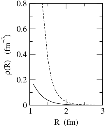
FIG. 5.: Dependence of the baryon density upon the cell radius for the “top” (solid) and “bottom” (dashed) solutions of set II.

FIG. 6.: Decomposition of the total energy (solid) into valence (dot) and vacuum (dashed) contributions, for the “top” solutions of set II (left panel) and III (right panel).

In Fig. 4 we plot the binding energy for the system taking out the spurious contributions stemming from the motion of the center of mass. In order to minimize the numerical uncertainty, the binding energy has been obtained by subtracting the total energy at the lowest considered density ($R=5$ fm). Interestingly, we find that, when the center-of-mass motion is taken out, a stronger minimum in the energy is found, roughly at the same density as in Fig. 4, namely $R\approx 1.8$ fm. Moreover, the boundary conditions of sets I and III provide more binding that those of set II. Note that in nuclear matter one should have a binding energy of about $-16$ MeV at $R\cong 1.1$ fm.

We also notice that the “top” solutions of the various sets of boundary conditions provide more binding than the corresponding “bottom” solutions. The reason is easily understood by looking, for example, at Fig. 6.

FIG. 7.: The ratio between the kinetic and potential components of the valence energy as a function of the cell radius, using the “top” boundary conditions of set II (solid) and set III (dashed).

FIG. 8.: Dependence of the pion decay constant on the the cell radius for the “top” solution of set II.

Here we plot the value of the baryon density at the surface of the cell, i.e. $u^{2}(R)+v^{2}(R)$, as a function of the cell radius itself, for the boundary conditions of set II (the solid and dashed lines corresponding to the top and bottom solutions respectively); sets I and III show a similar behavior. Since the top solution corresponds to a configuration in which the quarks are more “compressed” inside the cell, a larger kinetic energy, — and therefore a larger center-of-mass motion, — is associated with it. This problem is of course absent in solid state physics, the original field of application of the Wigner-Seitz approximation, because the electron mass is indeed completely negligible with respect to the mass of the ions, which form the periodic structure. In the present case, even admitting the existence of a periodic structure in nuclear matter, the center-of-mass motion would be neglegible only in the large $N_{c}$ limit ($N_{c}\rightarrow\infty$), given the dependence of the total energy and of the center-of-mass energy on the number of colors, as $O(N_{c})$ and $O(N_{c}^{0})$ respectively. On the other hand, for $N_{c}=3$, the center-of-mass energy will vary, for each solution inside the band, by an amount comparable with the width of the band itself. Hence, the calculation of a reliable band structure within this model is more delicate.

In Fig. 6 the total energy corresponding to the “top” solutions of set II (left) and III (right) is plotted, and decomposed into the valence (dotted) and vacuum (dashed) contributions. We observe that, at very low densities, the two components bear approximately the same strength, whereas at larger densities, below $R\cong 2$ fm, the valence contribution becomes dominant. It is also interesting to display, as a function of $R$, the ratio between the valence contributions that come from the quark kinetic term in the Lagrangian and from the quark coupling to the mean field. This is done in Fig. 8: As expected, this ratio increases with the density.

FIG. 9.: Isoscalar mean square radius, as a function of the cell radius. The solid line corresponds to the “top” solution of set II, whereas the dashed line corresponds to the “bottom” solution of Set III.

FIG. 10.: Chiral angle as a function of the distance from the center of the soliton for $R=5$ (solid), $2$ (dashed) and $1.1$ fm (dotted), respectively. The left panel corresponds to the “top” solution of set II, whereas the right one corresponds to the “top” solution of set III.

FIG. 11.: Large and small components of the Dirac spinor as a function of the distance from the center of the soliton for $R=5$ (solid), $2$ (dashed) and $1.1$ fm (dotted), respectively. The left panel corresponds to the “top” solution of set II, whereas the right one corresponds to the “top” solution of set III.

FIG. 12.: Baryon density as a function of the distance from the center of the soliton for $R=5$ (solid), $2$ (dashed) and $1.1$ fm (dotted), respectively. The left panel corresponds to the “top” solution of set II, whereas the right one corresponds to the “top” solution of set III.

FIG. 13.: The axial coupling constant as a function of $R$, for the “top” boundary conditions of set II (left panel) and set III (right panel). The valence (dashed), local mesonic (dotted), non-local mesonic (dot-dashed) and total (solid) contributions are displayed.

In Fig. 8 the average value of the pion decay constant in the cell, defined in Eq. (71), is plotted as a function of the cell radius, for the “top” solution of set II; for all the other sets of solutions the behavior is very similar. The pion decay constant decreases by increasing the density, going in the direction of a partial restoration of chiral symmetry, although the lack of solutions beyond roughly the standard saturation density of nuclear matter, prevents one, — at the present stage of development of the model, — from drawing firmer conclusions. A reduction of $f_{\pi}$ in matter is found both in linear sigma and Nambu-Jona-Lasinio models (see, e. g., Ref. [32] for a list of references).

In Fig. 10 the isoscalar mean radius is plotted as a function of the cell radius, for the “top” (solid) and “bottom” (dashed) solutions of set II; the other sets of solutions give very similar results. We observe that this quantity is extremely sensitive to the choice of “top” or “bottom” boundary conditions, the reason being the same as already noticed when discussing Fig. 6: The “bottom” solution in fact corresponds to a configuration in which the quarks are more loosely packed inside the cell. One could in principle define a mean radius averaged over the solutions distributed in the band, assuming, for instance, a uniform distribution. From Fig. 10 one would expect such an averaged radius to have a moderate density dependence. However, as already mentioned, we expect confinement to affect the band width, and expecially the “bottom” border (actually, the upper end), thus unbalancing the distribution in favor of the lower curve of Fig. 10 and yielding a shrinking of the soliton. This would be at variance with findings of other models.

For completeness we display in Figs. 10, 12 and 12, as a function of the distance from the center of the WS cell and for three values of $R$, the chiral angle, the large and the small components of the Dirac spinor and the baryon density, respectively, using the “top” solutions of sets II and III. Similar results apply for the other solutions.

A quantity which is more sensitive to the choice of boundary conditions is $g_{A}$, as one can see in Fig. 13. The local mesonic component varies noticeably in the different cases, even at large $R$. In Table III we display the value of the different components of $g_{A}$ at $R=5$ fm, compared to the results for the free soliton case. One clearly sees that the quark and non-local mesonic components have already reached the asymptotic value, whereas the local mesonic term is still higher. The reason for this behavior can be traced back to the slow decay of the chiral angle in the chiral limit ($\theta(r)\approx 1/r^{2}$), which allows sizeable contributions from large distances. Although in principle one could continue the WS calculation at larger radii, one would then need to increase the number of states included in the orthonormal basis employed in the expansion. However, it is likely that, when chiral symmetry is explicitly broken, the exponential decay of the chiral angle would grant a faster convergence and suppress the sensitivity to the boundary conditions. Increasing the density, the mesonic contributions to $g_{A}$, both local and non-local, rapidly decrease and most of the strength is now carried by the quarks alone.

TABLE II.:

	quark	local mesonic	non-local mesonic	total
free	1.07	0.50	-0.35	1.22
II	1.06	0.76	-0.34	1.48
III	1.06	1.03	-0.34	1.76

TABLE III.: The axial coupling constant $g_{A}$ in free space and in the Wigner-Seitz approximation at $R=5$ fm, for the “top” boundary conditions of sets II and III.

IV Outlook and perspectives

In this paper we have applied the Wigner-Seitz approximation to the chiral quark-soliton model of the nucleon. This model, complemented by the WS approximation, provides a simple yet interesting framework for studying possible modifications of the nucleon properties in nuclear matter. It is important to remark that we are actually dealing with a parameter-free model, since the only free parameters (the constituent quark mass $M$ and the regularization scale) have been fixed in free space. Note that $M$ could, in principle, be calculated dynamically, as done, e. g., in the Nambu-Jona-Lasinio model [2]; this would require the solution of a gap equation and would probably lead to an in-medium suppression of $M$, similar to what is found for $f_{\pi}$.

The same method of accounting for in-medium effects has already been applied to a number of microscopic models of the nucleon [13, 14, 15, 16, 17, 18, 19, 20, 21, 22, 23]. With respect to previous analyses, we have for the first time consistently calculated effects stemming from the Dirac sea, i. e., from excitations of virtual quark–antiquark pairs, including their dependence upon the density of the system.

Vacuum fluctuations manifest themselves in two ways. Firstly, by giving rise to a pion decay constant dependent on the distance from the center of the bag, which in turn modifies the pion kinetic contribution with respect to chiral models where the pion is explicitly included at the classical level [18, 19, 20, 17] (see Eqs. (41) and (42)): The contribution to the energy from this term is however qualitatively similar to the one of previous analyses [18, 19, 20, 17]. Secondly, vacuum fluctuations generate a new non-local, attractive contribution, whose density dependence, albeit moderate, is however relevant in order to bind the system, given the compensation one observes with increasing density between the valence quark and kinetic pion contributions.

Another effect that has usually been neglected in previous calculations is the spurious center-of-mass motion: We have found it to be important not only to give, of course, a more realistic estimate of the energy, but also to determine the relative position of the top and bottom ends of the quark energy band in the medium. These two levels correspond to specific boundary conditions and we have found the role of the boundary conditions generating the upper and lower levels to be exchanged with respect to previous calculations. Note that the intersection of an occupied band with an empty one is often interpreted as the onset of color superconductivity.

We have also explored the effects stemming from different choices of boundary conditions. All the cases discussed above display a similar qualitative behavior, although there are definitely quantitative differences, especially for the axial coupling constant, which is however very much affected by the long-range behavior of the chiral field in the (massless pion) chiral limit. Also the two regularization schemes we have adopted turned out to give qualitatively similar results.

We have calculated a few physical quantities, such as $f_{\pi}$ and $\langle r^{2}\rangle_{I=0}$. The pion decay constant has been found to decrease with increasing density, pointing to a partial restoration of chiral symmetry in the medium. The isoscalar mean square radius, on the other hand, has been found to depend heavily on the position in the energy band, leaving open the question whether an average nucleon will swell or shrink, given the present uncertainties in assessing the band structure.

Unlike previous calculations with chiral models [18, 19, 20, 17], we have been able to find binding, but at a density much lower than the standard saturation density of nuclear matter; moreover, solutions of the equations of motion disappear roughly below the latter density. The authors of Ref. [20] have been able to find solutions at high densities, — still keeping realistic values for the constituent quark mass parameter $M$, — by incorporating in their chiral Lagrangian terms of higher order in the pion field. In the present model this would correspond to dropping the two-point approximation to the effective action in evaluating vacuum fluctuations. This is probably the most needed development of the present calculation, — employing, e. g., the numerical algorithm of Ref. [33], — since only in the free case it has been explicitly verified that the two-point approximation works reasonably well [27].

Finally, another feature that is lacking at the present stage is the projection of good spin-isospin quantum numbers out of the hedgehog state. Since the momentum of inertia is, in general, density-dependent, the projection is likely to affect the position of the minimum in the energy.

A The propagator $K(q)$

We derive here the expression for the propagator $K(q)$, introduced in Sect. II B. As a first step we perform the angular integrals in Eq. (LABEL:eq:Kqr), getting

$$K(q) = \frac{1}{2\pi^{4}}\int_{0}^{\infty}dk\,k^{2}\int_{0}^{\infty}dk^{\prime}\,{k^{\prime}}^{2}\frac{\pi}{E_{k}E_{k^{\prime}}}\frac{C\left[\left(k+k^{\prime}\right)/2\right]}{E_{k}+E_{k^{\prime}}}\int_{0}^{\infty}dr\,r^{2}j_{0}(qr)j_{0}(kr)j_{0}(k^{\prime}r).$$ (A1)

The inner integral can be done analytically [34], yielding

$$\int_{0}^{\infty}dr\,r^{2}j_{0}(qr)j_{0}(kr)j_{0}(k^{\prime}r) = \left(\frac{\pi}{2}\right)^{3/2}\frac{1}{\sqrt{qkk^{\prime}}}\int_{0}^{\infty}dr\,\sqrt{r}J_{1/2}(qr)J_{1/2}(kr)J_{1/2}(k^{\prime}r)$$ (A2)

$$= \frac{\pi}{4}\frac{\Delta(q,k,k^{\prime})}{qkk^{\prime}},$$ (A3)

where the function $\Delta(x,y,z)$ vanishes whenever it is not possible to build a triangle of sides $x$, $y$ and $z$, and is equal to $1$ otherwise.

One then obtains

$$K(q)=\frac{1}{8\pi^{2}q}\int_{0}^{\infty}dk\,\frac{k}{E_{k}}\int_{|k-q|}^{k+q}dk^{\prime}\,\frac{k^{\prime}}{E_{k^{\prime}}}\frac{C\left[\left(k+k^{\prime}\right)/2\right]}{E_{k}+E_{k^{\prime}}}.$$ (A4)

B A basis for flat functions

In free space ($R\to\infty$) an orthonormal and complete set of states can be chosen as

$$\Psi_{k_{0}klm}(x)=\frac{1}{\pi}e^{ik_{0}x_{0}}Y_{l}^{m}(\Omega)j_{l}(kr).$$ (B1)

We want to build an orthonormal and complete basis inside a sphere of radius $R$, having the same form of (B1). While in that case the momentum could take a continuum set of values, now only a discrete set of momenta will be allowed.

We start considering the equations for the spherical Bessel functions, corresponding to two different momenta, $k_{1}=\alpha/R$ and $k_{2}=\beta/R$:

$$\frac{d}{dr}\left[r^{2}\frac{d}{dr}j_{l}\left(\frac{\alpha r}{R}\right)\right]+\left[\left(\frac{\alpha r}{R}\right)^{2}-l(l+1)\right]j_{l}\left(\frac{\alpha r}{R}\right) = 0$$ (B2)

$$\frac{d}{dr}\left[r^{2}\frac{d}{dr}j_{l}\left(\frac{\beta r}{R}\right)\right]+\left[\left(\frac{\beta r}{R}\right)^{2}-l(l+1)\right]j_{l}\left(\frac{\beta r}{R}\right) = 0.$$ (B3)

Multiplying both expressions by $j_{l}(\alpha r/R)$ and $j_{l}(\beta r/R)$, respectively, integrating over $r$ between $0$ and $R$, taking the difference of the two equations and, finally, integrating by parts, one gets

$$-\int_{0}^{R}\left(\alpha^{2}-\beta^{2}\right)\frac{r^{2}}{R^{2}}j_{l}\left(\frac{\alpha r}{R}\right)j_{l}\left(\frac{\beta r}{R}\right)=R\left[\alpha j^{\prime}_{l}(\alpha)j_{l}(\beta)-\beta j^{\prime}_{l}(\beta)j_{l}(\alpha)\right]$$ (B4)

The above equation states the orthonormality of the elements of the basis, provided that the following condition is met:

$$\alpha j^{\prime}_{l}(\alpha)j_{l}(\beta)-\beta j^{\prime}_{l}(\beta)j_{l}(\alpha)=0,\quad\alpha\neq\beta.$$ (B5)

The choice of the boundary conditions fulfilled by the elements of the basis will therefore be constrained by this requirement. It is easy to convince oneself that three different possibilities are available:

$$j_{l}(\alpha) = 0$$ (B7)

$$j_{l}^{\prime}(\alpha) = 0$$ (B8)

$$\alpha j_{l}^{\prime}(\alpha) = \eta j_{l}(\alpha),$$ (B9)

where $\eta$ will is a constant parameter. In the limit $\eta=0$ and $\eta\to\infty$ the first two cases are recovered, respectively.

Notice that, in the limit $R\to\infty$, — where the modes form a continuum, — all these boundary conditions become equivalent.

We then introduce the normalized functions

$$\rho_{\alpha_{l}}(r) \equiv \kappa_{\alpha_{l}}j_{l}\left(\frac{\alpha_{l}r}{R}\right)$$ (B10)

$$\kappa_{\alpha_{l}}^{2} = \frac{2}{R^{3}}\left[\alpha_{l}^{2}j_{l}^{\prime}(\alpha_{l})^{2}-j_{l}(\alpha_{l})\left(-2\alpha_{l}j_{l}^{\prime}(\alpha_{l})+(l(l+1)-\alpha_{l}^{2})j_{l}(\alpha_{l})\right)\right]^{-1},$$ (B11)

such that

$$\int_{0}^{R}dr\ r^{2}\rho_{\alpha_{l}}(r)\rho_{\beta_{l}}(r)=\delta_{\alpha_{l}\beta_{l}}.$$ (B12)

The completeness of the basis allows one to write the following representation for the Dirac delta function inside the WS cell:

$$\sum_{\alpha_{l}}\rho_{\alpha_{l}}(r)\rho_{\alpha_{l}}(r^{\prime})=\frac{\delta(r-r^{\prime})}{r^{2}}.$$ (B13)

It is simple to derive an expression for the Green’s function of the operator $(\Box+M^{2})$ in the WS cell. It reads

$$G(x,x^{\prime})=\sum_{l,m}\int_{-\infty}^{\infty}\frac{dk_{0}}{2\pi}\sum_{\alpha_{l}}Y_{l}^{m}(\Omega)Y_{l}^{m*}(\Omega^{\prime})e^{-ik_{0}(x_{0}-x^{\prime}_{0})}\frac{\rho_{\alpha_{l}}(r)\rho_{\alpha_{l}}(r^{\prime})}{\alpha_{l}^{2}/R^{2}+M^{2}-k_{0}^{2}}.$$ (B14)

The flat basis is obtained, as we said above, in the limit $\eta\to 0$; in this case, however, the lowest energy mode, — corresponding to zero momentum for $l=0$, can only be obtained for a strictly vanishing $\eta$ (in fact, it corresponds to a negative root of Eq. (B9) at finite values of $\eta$). This means that the strength of this mode has to be redistributed, for finite $\eta$, over all the other modes. Let us call $\beta$ and $\tilde{\beta}$ the modes such that

$$j^{\prime}_{l}(\beta)=0,\quad\tilde{\beta}j_{l}^{\prime}(\tilde{\beta})=\eta j_{l}(\tilde{\beta}).$$ (B15)

There is a one-to-one correspondence between the modes in the two bases, in such a way that for each $\beta\neq 0$ one can define $\tilde{\beta}=\beta-\epsilon_{\beta}$, where $\epsilon_{\beta}\ll 1$ if $\eta\ll 1$.

Writing down the transformation from one basis to the other, namely

$$\rho_{\beta}(r)=\sum_{\tilde{\beta}}c_{\beta\tilde{\beta}}\tilde{\rho}_{\tilde{\beta}}(r),$$ (B16)

with some algebra one can verify that, for $l=0$ and $\beta=0$, one has

$$c_{0\tilde{\beta}}=-\frac{\sqrt{6}}{\tilde{\beta}^{2}}\epsilon_{\beta},$$ (B17)

which indeed proves that the zero mode is now redistributed over all the other modes, in the quasi-flat basis.

Calculations in the two bases are equivalent (to order $\eta$) only when considering convergent quantities. Quantities that need regularization are therefore different in the two bases, since only a finite number of modes will contribute. The flat basis is the one we have chosen in the calculations of this paper, since it is the most convenient in order to impose the physically motivated boundary conditions discussed in the text. The zero mode, however, gives rise to divergences when $R\to 0$ and one could in principle eliminate this problem by employing a quasi-flat basis infinitesimally close to the flat one. On the other hand, the very fact that for regularized quantities only a finite number of modes is relevant, allows us to keep the flat basis and simply discard the zero mode, since the error introduced in this way will be infinitesimally small.

Finally, we display in Table IV a few simple rules that allow one to rewrite in the WS basis quantities expressed in the free basis (B1).

free space		Wigner-Seitz boundary conditions
$\int_{0}^{\infty}dk\ k^{2}$	$\longrightarrow$	$(\pi/2)\sum_{\alpha_{l}}$
$k$	$\longrightarrow$	$\alpha_{l}/R$
$j_{l}(kr)$	$\longrightarrow$	$\rho_{\alpha_{l}}(r)$

TABLE IV.: Rules for going from free space to the Wigner-Seitz cell.

REFERENCES

• [1] R. J. Bahduri, Models of the nucleon (Addison-Wesley, Reading, Massachusetts, 1988).
• [2] G. Ripka, Quarks bound by chiral fields (Clarendon Press, Oxford, 1997).
• [3] J. D. Walecka, Theoretical nuclear and subnuclear physics (Oxford University Press, Oxford, 1995).
• [4] D. I. Diakonov, V. Yu. Petrov, and P. V. Pobylitsa, Nucl. Phys. B306, 809 (1988).
• [5] D. I. Diakonov, V. Yu. Petrov, and M. Praszalowicz, Nucl. Phys. B323, 53 (1989).
• [6] M. Wakamatsu and H. Yoshiki, Nucl. Phys. A524, 561 (1991).
• [7] D. I. Diakonov, V. Yu. Petrov, and P. V. Pobylitsa, M. V. Polyakov, and C. Weiss, Phys. Rev. D 58, 038502 (1998).
• [8] E. M. Nyman, Nucl. Phys. B17, 599 (1970).
• [9] J. Achtzehnter, W. Scheid, and L. Wilets, Phys. Rev. D 32, 2414 (1985).
• [10] I. Klebanov, Nucl. Phys. B262, 133 (1985).
• [11] Q. Zhang, C. Derreth, A. Schäfer, and W. Greiner, J. Phys. G12, L19 (1986).
• [12] E. Wigner and F. Seitz, Phys. Rev. 43, 804 (1933).
• [13] E. Wust, G.E. Brown, and A.D. Jackson, Nucl.  Phys.  A468, 450 (1987).
• [14] P. Amore, Nuovo  Cimento  111A, 492 (1998).
• [15] H. Reinhardt, B. V. Dang, and H. Schulz, Phys. Lett. 159B, 161 (1985).
• [16] M. Birse, J. J. Rehr, and L. Wilets, Phys. Rev. C 38, 359 (1988).
• [17] U. Weber and J. A. McGovern, Phys. Rev. C 57, 3376 (1998).
• [18] B. Banerjee, N. K. Glendenning, and V. Soni, Phys. Lett. 155B, 213 (1985).
• [19] N. K. Glendenning and B. Banerjee, Phys. Rev. C 34, 1072 (1986).
• [20] D. Hahn and N. K. Glendenning, Phys. Rev. C 36, 1181 (1987).
• [21] C. W. Johnson, G. Fai, and M. R. Frank, Phys. Lett. B 386, 75 (1996).
• [22] C. W. Johnson and G. Fai, Phys. Rev. C 56, 3353 (1997).
• [23] C. W. Johnson and G. Fai, Heavy Ion Phys. 8, 343 (1998).
• [24] G. S. Adkins, C. R. Nappi, and E. Witten, Nucl. Phys. B228, 552 (1983).
• [25] I. J. R. Aitchison, C. M. Fraser, K. E. Tudor, and J. A. Zuk, Phys. Lett. 165B, 162 (1985).
• [26] S. Kahana and G. Ripka, Nucl. Phys. A429, 462 (1984).
• [27] I. Adjali, I. J. R. Aitchison, and J. A. Zuk, Nucl. Phys. A537, 457 (1992).
• [28] E. Elizalde, M. Bordag, and K. Kristen, J. Phys.  A31, 1743 (1998).
• [29] T. Kubota, M. Wakamatsu, and T. Watabe Phys. Rev. D 60, 014016 (1999).
• [30] T.D. Cohen and W. Broniowski, Phys. Rev. D 34, 3472 (1986).
• [31] P. V. Pobylitsa, E. Ruiz Arriola, T. Meissner, F. Grummer, K. Goeke, and W. Broniowski, J. Phys. G18, 1455 (1992).
• [32] M. C. Birse, J. Phys. G20, 1537 (1994).
• [33] S. Kahana and G. Ripka, Nucl. Phys. A429, 462 (1984).
• [34] I.S. Gradshteyn and I.M. Ryzhik, Table of integrals, series and products (Academic Press, New York, 1980).