Semiclassical transport of hadrons with dynamical spectral functions in $A+A$ collisions at SIS/AGS energies

Abstract

The transport of hadrons with dynamical spectral functions $A_{h}(X,\vec{P},M^{2})$ is studied for nucleus-nucleus collisions at SIS and AGS energies in comparison to the conventional quasi-particle limit and the available experimental data within the recently developed off-shell HSD transport approach. Similar to reactions at GANIL energies the off-shell effects show up in high momentum tails of the particle spectra, however, at SIS and AGS energies these modifications are found to be less pronounced than at lower energies due to the high lying excitations of the nucleons in the collision zone.

PACS: 24.10.Cn; 24.10.-i; 25.75.-q

Keywords: Many-body theory; Nuclear-reaction models and methods; Relativistic heavy-ion collisions

1 Introduction

Nowadays, the dynamical description of strongly interacting systems out of equilibrium is dominantly based on transport theories and efficient numerical recipies have been set up for the solution of the coupled channel transport equations [1, 2, 3, 4, 5, 6, 7] (and Refs. therein). These transport approaches have been derived either from the Kadanoff-Baym equations [8] in Refs. [9, 10, 11, 12, 13] or from the hierarchy of connected equal-time Green functions [14, 15] in Refs. [4, 16, 17] by applying a Wigner-transformation and restricting to first order in the derivatives of the phase-space variables ($X,P$).

However, as recognized early in these derivations [11, 16], the on-shell quasiparticle limit, that invoked additionally a reduction of the $8N$-dimensional phase-space to $7N$ independent degrees of freedom, where $N$ denotes the number of particles in the system, should not be adequate for particles with high collision rates (cf. also Refs. [18, 19]). Therefore, transport formulations for quasiparticles with dynamical spectral functions have been presented in the past [10, 12] providing a formal basis for an extension of the presently applied transport models denoted by BUU/VUU [2, 3, 20, 21, 22], QMD [23, 24, 25] or its relativistic versions RBUU [26], UrQMD [6], ART [27], ARC [28] or HSD [7, 29].

Recently, the authors have developed a semiclassical transport approach on the basis of the Kadanoff-Baym equations that includes the propagation of hadrons with dynamical spectral functions [30]. This approach has been examined for nucleus-nucleus collisions at GANIL energies and the off-shell propagation of nucleons and $\Delta$’s has lead to an enhancement of the high energy proton spectra as well as to an enhancement of high energy $\gamma$-rays rather well in line with related experimental studies. The question now arises whether such phenomena will also be encountered at SIS energies or AGS energies, i.e. at laboratory energies that are higher by one or two orders of magnitude, respectively.

The paper is organized as follows: In Section 2 we will briefly review the generalized transport equations on the basis of the Kadanoff-Baym equations [8], extend the test-particle representation to the general case of momentum-dependent self energies and specify the collision terms for bosons and fermions. Furthermore, we will present the mass differential cross sections for mesons from $NN$ and $\pi N$ collisions in the medium as well as the approximations for their ’collisional broadening’. The results for particle production in nucleus-nucleus collisions from the off-shell approach will be discussed in Section 3 in comparison to the quasi-particle limit as well as to the experimental data available. A summary and discussion of open problems concludes this study in Section 4.

2 Extended semiclassical transport equations

In this Section we briefly recall the basic equations for Green functions and particle self energies as well as their symmetry properties that will be exploited in the derivation of transport equations in the semiclassical limit.

The general starting point for the derivation of a transport equation for particles with finite width are the Dyson-Schwinger equations for the retarded and advanced Green functions $S^{ret}$, $S^{adv}$ and for the non-ordered Green functions $S^{<}$ and $S^{>}$ [30]. In the case of scalar bosons – which is considered in the following for simplicity – these Green functions are defined by

$$\hskip 56.9055pti\,S^{<}_{xy} := \;<\,\Phi^{\dagger}(y)\;\Phi(x)\,>\,,$$

$$i\,S^{>}_{xy} := \;<\,\Phi(x)\;\Phi^{\dagger}(y)\,>\,,$$

$$i\,S^{ret}_{xy} := \phantom{-}\>\Theta(x_{0}-y_{0})\,<\,[\,\Phi(x)\,,\,\Phi^{\dagger}(y)\,]\,>\,,$$

$$i\,S^{adv}_{xy} := -\>\Theta(y_{0}-x_{0})\,<\,[\,\Phi(x)\,,\,\Phi^{\dagger}(y)\,]\,>\,.$$ (1)

They depend on the space-time coordinates $x,y$ as indicated by the indices $\cdot_{xy}$. The Green functions are determined via Dyson-Schwinger equations by the retarded and advanced self energies $\Sigma^{ret},\Sigma^{adv}$ and the collisional self energy $\Sigma^{<}$:

$$\hat{S}_{0x}^{-1}\;S_{xy}^{ret}\;\>=\;\>\delta_{xy}\;\>+\;\>\Sigma_{xz}^{ret}\>\odot\>S_{zy}^{ret}\;,$$ (2)

$$\hat{S}_{0x}^{-1}\;S_{xy}^{adv}\;\>=\;\>\delta_{xy}\;\>+\;\>\Sigma_{xz}^{adv}\>\odot\>S_{zy}^{adv}\;,$$ (3)

$$\hat{S}_{0x}^{-1}\;S_{xy}^{<}\;\>=\;\>\Sigma_{xz}^{ret}\>\odot\>S_{zy}^{<}\;\>+\;\>\Sigma_{xz}^{<}\>\odot\>S_{zy}^{adv}\>.$$ (4)

Equation (4) is the well-known Kadanoff-Baym equation. Here $\hat{S}^{-1}_{0x}$ denotes the (negative) Klein-Gordon differential operator which is given for bosonic field quanta of (bare) mass $M_{0}$ by $\hat{S}^{-1}_{0x}=-(\partial^{\mu}_{x}\partial^{x}_{\mu}+M^{2}_{0})$, $\delta_{xy}$ represents the four-dimensional $\delta$-distribution $\delta_{xy}\equiv\delta^{(4)}(x-y)$ and the symbol $\odot$ indicates an integration (from $-\infty$ to $\infty$) over all common intermediate variables (cf. [30]).

For the derivation of a semiclassical transport equation one now changes from a pure space-time formulation into the Wigner-representation. The theory is then formulated in terms of the center-of-mass variable $X=(x+y)/2$ and the momentum $P$, which is introduced by Fourier-transformation with respect to the relative space-time coordinate $(x-y)$. In any semiclassical transport theory it is furthermore assumed that the dependence on the mean space-time coordinates $X$ of all functions is rather weak. Therefore, in the Wigner-transformed expressions only contributions up to the first order in the space-time gradients are kept. After carrying-out these two steps the Dyson-Schwinger equations (2-4) become

$$\left[\,P^{2}\,-\,M^{2}_{0}\,+\,iP^{\mu}\partial^{X}_{\mu}\,\right]\>S^{ret}_{XP}\;=\;1\>+\>(\,1\,-\,i\,\Diamond\,)\,\{\,\Sigma^{ret}_{XP}\,\}\>\{\,S^{ret}_{XP}\,\}\>,$$ (5)

$$\left[\,P^{2}\,-\,M^{2}_{0}\,+\,iP^{\mu}\partial^{X}_{\mu}\,\right]\>S^{adv}_{XP}\;=\;1\>+\>(\,1\,-\,i\,\Diamond\,)\,\{\,\Sigma^{adv}_{XP}\,\}\>\{\,S^{adv}_{XP}\,\}\>,$$ (6)

$$\left[\,P^{2}\,-\,M^{2}_{0}\,+\,iP^{\mu}\partial^{X}_{\mu}\,\right]\>S^{<}_{XP}\;=\;(\,1\,-\,i\,\Diamond\,)\,\left[\>\{\,\Sigma^{ret}_{XP}\,\}\>\{\,S^{<}_{XP}\,\}\;+\;\{\,\Sigma^{<}_{XP}\,\}\>\{\,S^{adv}_{XP}\,\}\>\right].$$ (7)

The operator $\Diamond$ is defined as [12, 30]

$$\Diamond\,\{\,F_{1}\,\}\,\{\,F_{2}\,\}\;:=\;\frac{1}{2}\left(\frac{\partial F_{1}}{\partial X^{\mu}}\>\frac{\partial F_{2}}{\partial P_{\mu}}\;-\;\frac{\partial F_{1}}{\partial P_{\mu}}\>\frac{\partial F_{2}}{\partial X^{\mu}}\right),$$ (8)

which is a four-dimensional generalization of the well-known Poisson-bracket. Starting from (5) and (6) one obtains algebraic relations between the real and the imaginary part of the retarded Green functions. On the other hand eq. (7) leads to a ’transport equation’ for the Green function $S^{<}$.

We briefly recall the necessary steps: we separate all retarded and advanced quantities – Green functions and self energies – into real and imaginary parts,

$$S_{XP}^{ret,adv}\;=\;ReS^{ret}_{XP}\;\mp\;\frac{i}{2}\,A_{XP}\;,\qquad\Sigma_{XP}^{ret,adv}\;=\;Re\Sigma^{ret}_{XP}\;\mp\;\frac{i}{2}\,\Gamma_{XP}\;.$$ (9)

The imaginary part of the retarded propagator is given (up to a factor 2) by the normalized spectral function

$$A_{XP}\>=\>i\left[\,S_{XP}^{ret}\>-\>S_{XP}^{adv}\,\right]\>=\>-2\,Im\,S^{ret}_{XP}\;,\qquad\qquad\qquad\int\frac{dP_{0}^{2}}{4\pi}\,A_{XP}\;=\;1\;,$$ (10)

while the imaginary part of the self energy corresponds to half the width $\Gamma_{XP}$. By separating the complex equations (5) and (6) into their real and imaginary contributions we obtain an algebraic equation between the real and the imaginary part of $S^{ret}$,

$$ReS^{ret}_{XP}\;=\;\frac{P^{2}\>-\>M_{0}^{2}\>-\>Re\Sigma^{ret}_{XP}}{\Gamma_{XP}}\;A_{XP}\,.$$ (11)

In addition we gain an algebraic solution for the spectral function (in first order gradient expansion) as

$$A_{XP}\;=\;\frac{\Gamma_{XP}}{(\,P^{2}\,-\,M_{0}^{2}\,-\,Re\Sigma^{ret}_{XP})^{2}\>+\>\Gamma_{XP}^{2}/4}\;,$$ (12)

while the real part of the retarded propagator is given by

$$ReS^{ret}_{XP}\;=\;\frac{P^{2}\>-\>M_{0}^{2}\>-\>Re\Sigma^{ret}_{XP}}{(\,P^{2}\,-\,M_{0}^{2}\,-\,Re\Sigma^{ret}_{XP})^{2}\>+\>\Gamma_{XP}^{2}/4}\,.$$ (13)

Furthermore, the (Wigner-transformed) Kadanoff-Baym equation (7) allows for the construction of a transport equation for the Green function $S^{<}$. When separating the real and the imaginary contribution of this equation we find i) a generalized transport equation,

$$\Diamond\,\{\,P^{2} - M_{0}^{2}\>-\>Re\Sigma^{ret}_{XP}\,\}\;\{\,S^{<}_{XP}\,\}\;-\;\Diamond\,\{\,\Sigma^{<}_{XP}\,\}\;\{ReS^{ret}_{XP}\,\}$$ (14)

$$= \frac{i}{2}\>\left[\>\Sigma^{>}_{XP}\>S^{<}_{XP}\;-\;\Sigma^{<}_{XP}\>S^{>}_{XP}\>\right],$$

and ii) a generalized mass-shell constraint

$$[\,P^{2} - M_{0}^{2}\>-\>Re\Sigma^{ret}_{XP}\,]\;S^{<}_{XP}\;-\;\Sigma^{<}_{XP}\;ReS^{ret}_{XP}$$ (15)

$$= \frac{1}{2}\,\Diamond\;\{\,\Sigma^{<}_{XP}\,\}\;\{\,A_{XP}\,\}\;-\;\frac{1}{2}\,\Diamond\;\{\,\Gamma_{XP}\,\}\;\{\,S^{<}_{XP}\,\}\;.$$

We note that so far no reduction to the quasiparticle limit has been introduced. Besides the drift term (i.e. $\Diamond\{P^{2}-M^{2}_{0}\}\{S^{<}\}=-P^{\mu}\partial^{X}_{\mu}S^{<})$ and the Vlasov term (i.e. $\Diamond\{Re\Sigma^{ret}\}\{S^{<}\}$) a third contribution appears on the l.h.s. of (14) (i.e. $\Diamond\{\Sigma^{<}\}\{ReS^{ret}\}$), which vanishes in the quasiparticle limit and incorporates – as shown in [30] – the off-shell behaviour in the particle propagation. It is worth to point out that this particular term has been discarded in Ref. [31] and an off-shell propagation had to be introduced by hand via some mass-dependent real potential. To our best knowledge, such an auxiliary potential cannot be extracted from the Kadanoff-Baym equation (4). The r.h.s. of (14) consists of a collision term with its characteristic gain ($\sim\Sigma^{<}S^{>}$) and loss ($\sim\Sigma^{>}S^{<}$) structure, where scattering processes of particles into and out off a given phase-space cell are described.

Within the specific term ($\Diamond\{\Sigma^{<}\}\{ReS^{ret}\}$) a further modification is necessary. According to Botermans and Malfliet [10] the collisional self energy $\Sigma^{<}$ should be replaced by $S^{<}\cdot\Gamma/A$ to gain a consistent first order gradient expansion scheme. The replacement is allowed since the difference between these two expressions can be shown to be of first order in the space-time gradients itself. Therefore it has to be discarded when appearing inside an additional Poisson-bracket. Furthermore, this substitution is required to get rid of the inequivalence between the general transport equation and the general mass shell constraint which is present in (14) and (15) [18] but vanishes by invoking $S^{<}\cdot\Gamma/A$. Finally, the general transport equation (in first order gradient expansion) reads [30]

$$A_{XP}\,\Gamma_{XP} \!\!\!\!\!\!\!\!\!\!\left[\,\Diamond\;\{\,P^{2}-M_{0}^{2}-Re\Sigma^{ret}_{XP}\,\}\;\{\,S^{<}_{XP}\,\}\>-\>\frac{1}{\Gamma_{XP}}\;\Diamond\;\{\,\Gamma_{XP}\,\}\;\{\,(\,P^{2}-M_{0}^{2}-Re\Sigma^{ret}_{XP}\,)\,S^{<}_{XP}\,\}\,\right]$$ (16)

$$\;=\;i\,\left[\,\Sigma^{>}_{XP}\>S^{<}_{XP}\>-\>\Sigma^{<}_{XP}\>S^{>}_{XP}\,\right].$$

Its formal structure is fixed by the approximations applied. Note, however, that the dynamics is fully determined by the different self energies, i.e. $Re\Sigma_{XP}^{ret},\Gamma_{XP},\Sigma_{XP}^{<}$ and $\Sigma_{XP}^{>}$ that have to be specified for the physical systems of interest.

2.1 Testparticle representation

In order to obtain an approximate solution to the transport equation (16) we use a testparticle ansatz for the Green function $S^{<}$, more specifically for the real and positive semidefinite quantity

$$F_{XP}\;=A_{XP}N_{XP}=\;i\,S^{<}_{XP}\;\sim\;\sum_{i=1}^{N}\;\delta^{(3)}({\vec{X}}\,-\,{\vec{X}}_{i}(t))\;\;\delta^{(3)}({\vec{P}}\,-\,{\vec{P}}_{i}(t))\;\;\delta(P_{0}-\,\epsilon_{i}(t))\>.$$ (17)

Whereas so far we have briefly repeated the derivation from [30], we now extend the testparticle description to explicitly four-momentum-dependent self energies. The latter is not essential for the description of low and intermediate energy heavy-ion reactions, but becomes necessary for relativistic dynamics. In the most general case (where the self energies depend on four-momentum $P$, time $t$ and the spatial coordinates $\vec{X}$) the equations of motion for the testparticles read

$$\frac{d{\vec{X}}_{i}}{dt}\! = \!\phantom{-}\frac{1}{1-C_{(i)}}\,\frac{1}{2\epsilon_{i}}\>\left[\,2\,{\vec{P}}_{i}\,+\,{\vec{\nabla}}_{P_{i}}\,Re\Sigma^{ret}_{(i)}\,+\,\frac{\epsilon_{i}^{2}-{\vec{P}}_{i}^{2}-M_{0}^{2}-Re\Sigma^{ret}_{(i)}}{\Gamma_{(i)}}\>{\vec{\nabla}}_{P_{i}}\,\Gamma_{(i)}\>\right],$$ (18)

$$\frac{d{\vec{P}}_{i}}{dt}\! = \!-\frac{1}{1-C_{(i)}}\,\frac{1}{2\epsilon_{i}}\>\left[{\vec{\nabla}}_{X_{i}}\,Re\Sigma^{ret}_{i}\>+\>\frac{\epsilon_{i}^{2}-{\vec{P}}_{i}^{2}-M_{0}^{2}-Re\Sigma^{ret}_{(i)}}{\Gamma_{(i)}}\>{\vec{\nabla}}_{X_{i}}\,\Gamma_{(i)}\>\right],$$ (19)

$$\frac{d\epsilon_{i}}{dt}\! = \!\phantom{-}\frac{1}{1-C_{(i)}}\,\frac{1}{2\epsilon_{i}}\>\left[\frac{\partial Re\Sigma^{ret}_{(i)}}{\partial t}\>+\>\frac{\epsilon_{i}^{2}-{\vec{P}}_{i}^{2}-M_{0}^{2}-Re\Sigma^{ret}_{(i)}}{\Gamma_{(i)}}\>\frac{\partial\Gamma_{(i)}}{\partial t}\right],$$ (20)

where the notation $F_{(i)}$ implies that the function is taken at the coordinates of the testparticle, i.e. $F_{(i)}\equiv F(t,\vec{X}_{i}(t),\vec{P}_{i}(t),\epsilon_{i}(t))$.

In (18-20) a common multiplication factor $(1-C_{(i)})^{-1}$ appears, which contains the energy derivatives of the retarded self energy

$$C_{(i)}\>=\>\frac{1}{2\epsilon_{i}}\left[\frac{\partial}{\partial\epsilon_{i}}\,Re\Sigma^{ret}_{(i)}\>+\>\frac{\epsilon_{i}^{2}-{\vec{P}}_{i}^{2}-M_{0}^{2}-Re\Sigma^{ret}_{(i)}}{\Gamma_{(i)}}\>\frac{\partial}{\partial\epsilon_{i}}\,\Gamma_{(i)}\right]\>.$$ (21)

It yields a shift of the system time $t$ to the ’eigentime’ of particle $i$ defined by $\tilde{t}_{i}=t/(1-C_{(i)})$. As the reader immediately verifies, the derivatives with respect to the ’eigentime’, i.e. $d\vec{X}_{i}/d\tilde{t}_{i}$, $d\vec{P}_{i}/d\tilde{t}_{i}$ and $d\epsilon_{i}/d\tilde{t}_{i}$ then emerge without this renormalization factor for each testparticle $i$ when neglecting higher order time derivatives in line with the semiclassical approximation scheme. The role and the importance of this correction factors will be studied in detail for a four-momentum-dependent ’trial’ potential in Section 2.2. We note that for momentum-independent self energies we regain the transport equations as derived in [30]; only in case of particles with a vanishing vacuum width $\Gamma_{V}$ = 0 and $\Gamma_{XP}\sim\rho_{B}$ (baryon density) these equations reduce to the ’ad hoc’ assumptions introduced in Ref. [31]. Furthermore, in the limiting case of particles with vanishing gradients of the width $\Gamma_{XP}$ these equations of motion reduce to the well-known transport equations of the quasiparticle picture.

Following Ref. [30] we take $M^{2}=P^{2}-Re\Sigma^{ret}$ as an independent variable instead of $P_{0}$, which then fixes the energy (for given $\vec{P}$ and $M^{2}$) to

$$P_{0}^{2}\;=\;\vec{P}^{2}\>+\>M^{2}\>+\>Re\Sigma_{X\vec{P}M^{2}}^{ret}\,.$$ (22)

Eq. (20) then turns to

$$\frac{dM_{i}^{2}}{dt}\;=\;\frac{M_{i}^{2}-M_{0}^{2}}{\Gamma_{(i)}}\;\frac{d\Gamma_{(i)}}{dt}$$ (23)

for the time evolution of the test-particle $i$ in the invariant mass squared as derived in Ref. [30].

We briefly comment that in Ref. [30] we have added a term $\sim\partial\Gamma_{(i)}/\partial t$ in the equation of motion for the test-particle momenta in order to achieve strict energy conservation for each test-particle; however, within the subsequent approximations introduced in the actual transport calculations for energetic nucleus-nucleus collisions such a term did not lead to noticable effects within the numerical accuracy achieved. We thus discard such a term in the present formulation and investigation.

2.2 Model simulations for the momentum-dependent transport equations in testparticle representation

To demonstrate the physical content of the equations of motion for testparticles (18-20) we perform an exploratory study with a momentum-dependent trial potential. The potential is chosen of the type:

$$Re\Sigma^{ret}-\frac{i}{2}\Gamma\>=\>\frac{V(P_{0},\vec{P})}{1+\exp\{(|\vec{r}|-R)/a_{0}\}}\;-\;i\left(\frac{W(P_{0},\vec{P})}{1+\exp\{(|\vec{r}|-R)/a_{0}\}}\>+\>\frac{\Gamma_{V}}{2}\right)$$ (24)

with a constant (but finite) vacuum width $\Gamma_{V}$. While the spatial extension of the potential is given (as in [30]) by a Woods-Saxon shape (with parameters $R=5$ fm and $a_{0}=0.6$ fm) its momentum dependence for the real as well as for the imaginary part is introduced by

$$V(P_{0},\vec{P})\;\;=C_{V}\>\frac{\Lambda_{V}^{2}}{\Lambda_{V}^{2}-(P_{0}^{2}-\vec{P}^{2})}\>,\qquad W(P_{0},\vec{P})\;\;=C_{W}\>\frac{\Lambda_{W}^{2}}{\Lambda_{W}^{2}-(P_{0}^{2}-\vec{P}^{2})}\>.$$ (25)

Here the constants $C_{V}$ ($C_{W}$) give the ’strength’ of the complex potential while $\Lambda_{V}$ ($\Lambda_{W}$) play the role of cutoff-parameters. Due to the structure in the denominator of (25) the momentum-dependent part of this potential is explicitly Lorentz-covariant.

In our simulation we propagate the testparticles with different initial mass parameters $M_{i}$, which are shifted relative to each other by $\Gamma_{V}/(20$ GeV) around a mean mass of 1.0 GeV. To each testparticle a momentum in positive $z$-direction is attributed so that all of them have initially the same energy $P_{0}$ = 2.0 GeV. All testparticles are initialized on the negative $z$-axis with ($|\vec{X}_{i}(t=0)|\approx 15$ fm) and then evolved in time according to the equations of motion (18-20).

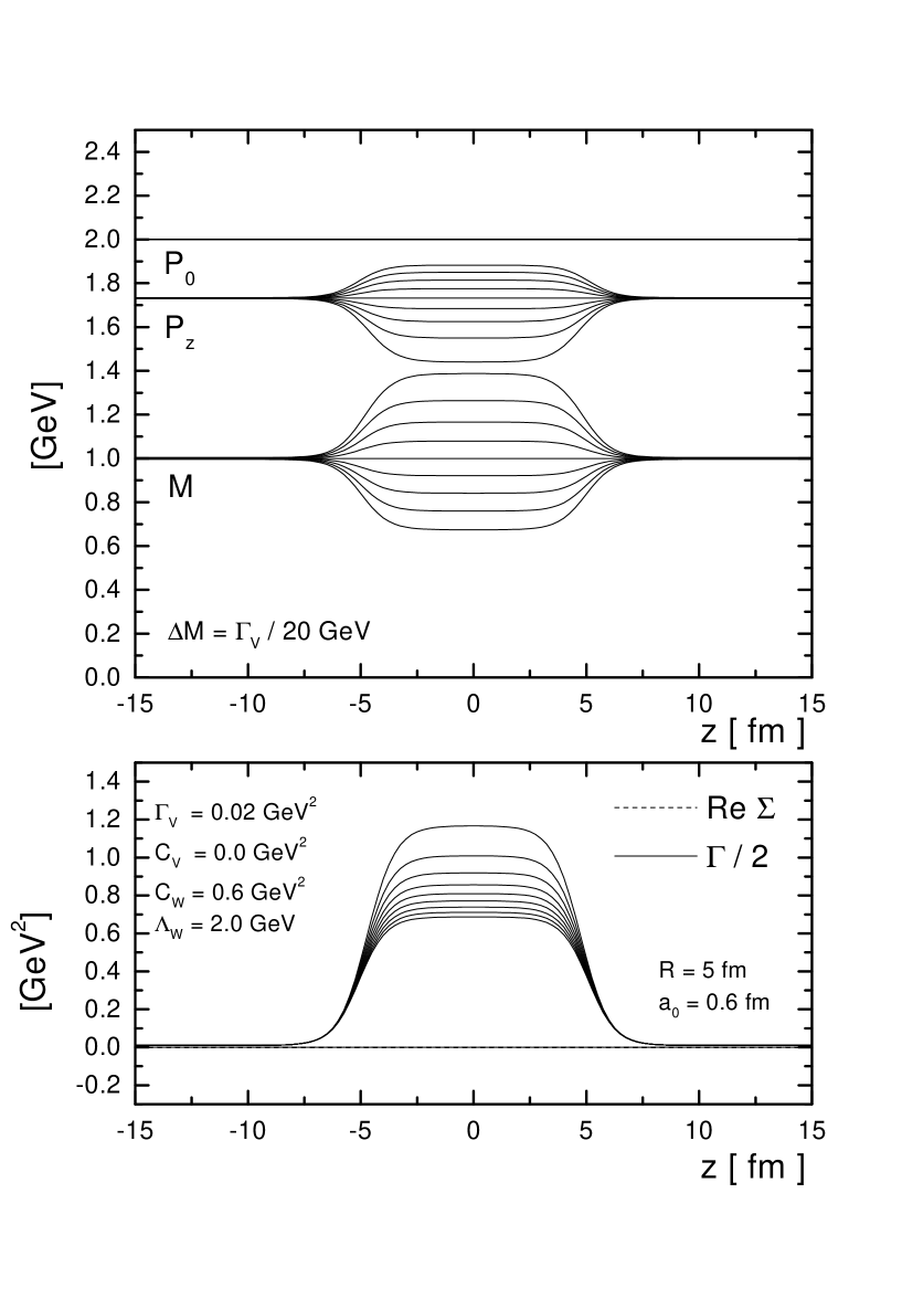
Figure 1: upper part: $P_{i0}$, $P_{iz}$ and $M_{i}$ as a function of $z(t)$ for a momentum-dependent imaginary potential with $C_{W}=0.6$ GeV² and $\Lambda_{W}=2.0$ GeV (lower part). The vacuum width is chosen as $\Gamma_{V}=0.02$ GeV² and the initial separation in the mass parameter of the testparticles is $\Delta M=\Gamma_{V}/20$.

In our first simulation we consider a purely imaginary potential with a strength of $C_{W}=0.6$ GeV² and a cutoff-parameter $\Lambda_{W}=2.0$ GeV. The evolution in energy $P_{0i}$, momentum $P_{zi}$ and in the mass parameter $M_{i}$ for all testparticles is shown in Fig. 1 (upper part) as a function of $z(t)$. When the testparticles enter the potential region, their momenta and mass parameters are modified. As already shown in [30] the imaginary potential leads to a spreading of the trajectories in the mass parameter $M_{i}$ which in turn reflects a broadening of the spectral function. The relation between the imaginary self energy and the spreading in mass is fully determined by relation (23). Since we have chosen a potential with no explicit time dependence the energy of each testparticle is a constant of time (cf. Ref. [30]). According to the explicit momentum dependence of our ’trial’ potential each single testparticle is affected with different strength. Since the imaginary potential is strongest for small momenta (which correspond to the highest lines in the lower graph of Fig. 1) the momentum and mass coordinates of those testparticles are changed predominantly that are initialized with the lowest momenta (i.e. with the largest masses). As a result one observes a rather asymmetric distribution in the mass parameters (and in the momenta) in the potential zone. This is different from the studies of [30] where the investigated momentum-independent potential yields a nearly equidistant spreading of the mass trajectories. For $z(t)\gg R$ the mass and momentum coordinates of the testparticles return to the proper asymptotic value.

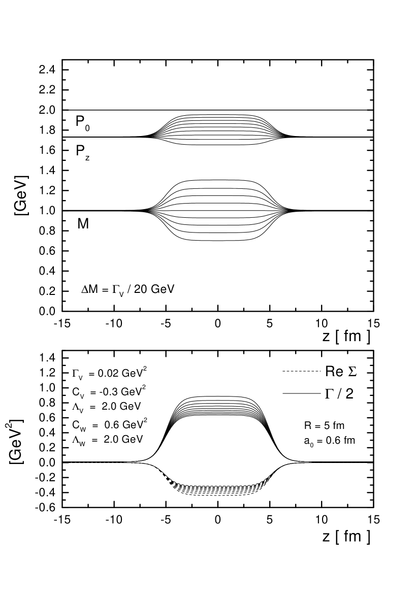
Figure 2: upper part: $P_{i0}$, $P_{iz}$ and $M_{i}$ as a function of $z(t)$ for a momentum-dependent complex potential with $C_{V}=-0.3$ GeV², $\Lambda_{V}=2.0$ GeV, $C_{W}=0.6$ GeV² and $\Lambda_{W}=2.0$ GeV (lower part). For the vacuum width and the initial mass separation the same values are used as in Fig. 1.

In the second example we allow for an addititonal real part of the self energy. The calculation is performed with the parameters $C_{V}=-0.3$ GeV², $C_{W}=0.6$ GeV² and $\Lambda_{V}=\Lambda_{W}=2.0$ GeV. The momentum-dependent real part (lower part of Fig. 2) causes – as also observed in [30] – an additional shift of the testparticle momenta. Since the real part of the potential is larger for small initial momenta, these testparticle momenta are shifted up somewhat more than for particles with larger momenta. This gives rise to a reduction of the asymmetry which was introduced by the momentum-dependent imaginary part of the self energy (upper part of Fig. 2). As in [30] the mass parameters of the testparticles are only weakly influenced by the real part of the potential.

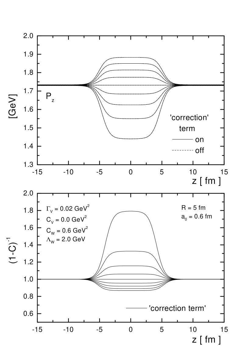
Figure 3: lower part: Correction term $(1-C_{(i)})^{-1}$ as a function of $z(t)$ for the same imaginary potential as in Fig. 1. Upper part: $P_{iz}$ as a function of $z(t)$ with and without including of the correction term. Both curves cannot be resolved separately within the line width.

We, furthermore, study the implications of the correction term $(1-C_{(i)})^{-1}$ using the same imaginary potential as in Fig. 1. The time evolution of the correction factor for each testparticle $i$ is displayed in the lower part of Fig 3. While it is $>1$ for large initial mass parameters $M_{i}>M_{0}$, it is $<1$ for mass parameters $M_{i}<M_{0}$. In the upper part of Fig. 3 the momenta of the testparticles are shown for two calculational limits: in the first one the correction term is taken into account (as in the previous calculations), while in the second one the corrections due to the energy dependence of the retarded self energy are neglected. However, the calculations with and without the correction factor exhibit only a very small difference in the testparticle momenta, which even cannot be distinguished within the resolution of Fig. 3. The same holds for the mass parameters $M_{i}$ which are not displayed here since they provide no new information due to energy conservation. We thus conclude that the particle trajectory is not very sensitive to these correction factors, since the correction term – when displayed as $P_{z}(z)$ in phase-space – leads only to a rescaling of the ’eigentime’ of the testparticles as pointed out before.

2.3 Collision terms

The collision term of the Kadanoff-Baym equation can only be worked out in more detail by giving explicit approximations for $\Sigma^{<}$ and $\Sigma^{>}$. A corresponding collision term can be formulated in full analogy to Refs. [3, 16], e.g. from Dirac-Brueckner theory, and implementing detailed balance as

$$I_{coll}(X,\vec{P},M^{2})=Tr_{2}Tr_{3}Tr_{4}A(X,{\vec{P}},M^{2})A(X,{\vec{P}}_{2},M_{2}^{2})A(X,{\vec{P}}_{3},M_{3}^{2})A(X,{\vec{P}}_{4},M_{4}^{2})$$

$$|T(({\vec{P}},M^{2})+({\vec{P}}_{2},M_{2}^{2})\rightarrow({\vec{P}}_{3},M_{3}^{2})+({\vec{P}}_{4},M_{4}^{2}))|_{{\cal A,S}}^{2}\;\;\delta^{(4)}({P}+{P}_{2}-{P}_{3}-{P}_{4})$$

$$[\,N_{X{\vec{P}}_{3}M_{3}^{2}}\,N_{X{\vec{P}}_{4}M_{4}^{2}}\,{\bar{f}}_{X{\vec{P}}M^{2}}\,{\bar{f}}_{X{\vec{P}}_{2}M_{2}^{2}}\>-\>N_{X{\vec{P}}M^{2}}\,N_{X{\vec{P}}_{2}M_{2}^{2}}\,{\bar{f}}_{X{\vec{P}}_{3}M_{3}^{2}}\,{\bar{f}}_{X{\vec{P}}_{4}M_{4}^{2}}\,]$$ (26)

with

$${\bar{f}}_{X{\vec{P}}M^{2}}=1+\eta\,N_{X{\vec{P}}M^{2}}$$ (27)

and $\eta=\pm 1$ for bosons/fermions, respectively. The indices ${\cal A,S}$ stand for the antisymmetric/symmetric matrix element of the in-medium scattering amplitude $T$ in case of fermions/bosons. In eq. (26) the trace over particles 2,3,4 reads explicitly for fermions

$$Tr_{2}=\sum_{\sigma_{2},\tau_{2}}\frac{1}{(2\pi)^{4}}\int d^{3}P_{2}\frac{dM^{2}_{2}}{2\sqrt{\vec{P}^{2}_{2}+M^{2}_{2}}},$$ (28)

where $\sigma_{2},\tau_{2}$ denote the spin and isospin of particle 2. In case of bosons we have

$$Tr_{2}=\sum_{\sigma_{2},\tau_{2}}\frac{1}{(2\pi)^{4}}\int d^{3}P_{2}\frac{dP_{0,2}^{2}}{2},$$ (29)

since here the spectral function $A_{B}$ is normalized as

$$\int\frac{dP_{0}^{2}}{4\pi}A_{B}(X,P)=1$$ (30)

whereas for fermions we have

$$\int\frac{dP_{0}}{2\pi}A_{F}(X,P)=1.$$ (31)

We mention that the spectral function $A_{F}$ in case of fermions in (26) is obtained by considering only particles of positive energy and assuming the spectral function to be identical for spin ’up’ and ’down’ states. In general, the spectral function for fermions ${\hat{A}}_{\alpha\beta}(X,P)$ is a Dirac-tensor with $\alpha\beta$ denoting the Dirac indices. It is normalized as

$$\int\frac{dP_{0}}{2\pi}{\hat{A}}_{\alpha\beta}(X,P)=(\gamma^{0})_{\alpha\beta},$$ (32)

which implies

$$\frac{1}{4}\sum_{\alpha}\int\frac{dP_{0}}{2\pi}(\gamma^{0}{\hat{A}}(X,P))_{\alpha\alpha}=1.$$ (33)

Now expanding ${\hat{A}}$ in terms of free spinors $u_{s}(P)$ ($s$=1,2) and $v_{s}(P)$ as

$$(\hat{A})_{\alpha\beta}\>=\>\sum_{r,s=1}^{2}\bar{u}_{s}(\vec{P}_{,}M)_{\beta}\;A_{rs}^{p}\;u_{r}(\vec{P},M)_{\alpha}\>+\>\bar{v}_{s}(\vec{P}_{,}M)_{\beta}\;A_{rs}^{ap}\;v_{r}(\vec{P},M)_{\alpha}$$ (34)

one can separate particles and antiparticles. By neglection of the antiparticle contributions (i.e. $A_{rs}^{ap}\equiv 0$) and within the assumption that the spectral function for the particles is diagonal in spin-space (i.e. $A_{rs}^{p}=\delta_{rs}A_{s}^{p}$) as well as spin symmetric, one can define $A_{F}$ as

$$A_{F}\equiv A_{1}^{p}=A_{2}^{p}\>.$$ (35)

Neglecting the ’gain-term’ in eq. (26) one recognizes that the collisional width of the particle in the rest frame is given by

$$\Gamma_{coll}(X,\vec{P},M^{2})=Tr_{2}Tr_{3}Tr_{4}\;|T(({\vec{P}},M^{2})+({\vec{P}}_{2},M_{2}^{2})\rightarrow({\vec{P}}_{3},M_{3}^{2})+({\vec{P}}_{4},M_{4}^{2}))|_{{\cal A,S}}^{2}$$ (36)

$$A(X,{\vec{P}}_{2},M_{2}^{2})A(X,{\vec{P}}_{3},M_{3}^{2})A(X,{\vec{P}}_{4},M_{4}^{2})\;\;\delta^{4}(P+P_{2}-P_{3}-P_{4})\ N_{X{\vec{P}}_{2}M_{2}^{2}}\,{\bar{f}}_{X{\vec{P}}_{3}M^{2}_{3}}\,{\bar{f}}_{X{\vec{P}}_{4}M^{2}_{4}}\,,$$

where as in eq. (26) local on-shell scattering processes are assumed for the transitions $P+P_{2}\rightarrow P_{3}+P_{4}$. We note that the extension of eq. (26) to inelastic scattering processes (e.g. $NN\rightarrow N\Delta$) or ($\pi N\rightarrow\Delta$ etc.) is straightforward when exchanging the elastic transition amplitude $T$ by the corresponding inelastic one and taking care of Pauli-blocking or Bose-enhancement for the particles in the final state. We note that for bosons we will neglect a Bose-enhancement factor throughout this work since their actual phase-space density is small for the systems of interest.

For particles of infinite life time in vacuum – such as protons – the collisional width (36) has to be identified with twice the imaginary part of the self energy. Thus the transport approach determines the particle spectral function dynamically via (36) for all hadrons if the in-medium transition amplitudes $T$ are known in their full off-shell dependence. Since this information is not available for configurations of hot and dense matter, which is the major subject of future development, a couple of assumptions and numerical approximation schemes have to be invoked in actual applications.

2.4 Numerical realization

As in Ref. [30] the following dynamical calculations are based on the conventional HSD transport approach [7, 29] – in which $Re\Sigma^{ret}_{XP}$ is specified for the hadrons – however, the equations of motion for the testparticles are extended to (18,19,23). Whereas for energies up to 100 A MeV (GANIL energies) essentially the nucleon degrees of freedom were important [30] we have to specify the actual ’recipies’ for nucleon and meson resonances involved in the following calculations.

As a first approximation we only consider reactions with binary channels which for convenience can be described in their center-of-mass (cms) frame. The collisions of nucleons (as well as all hadrons) are described by the closest distance criterion of Kodama et al. [32]: a collision of two particles takes place only if their distance in the individual cms is small enough, i.e.

$$|{\vec{X}}_{1}-{\vec{X}}_{2}|\leq\sqrt{\sigma({|\vec{P}}_{1}-{\vec{P}}_{2}|)/\pi},$$ (37)

where $\sigma$ denotes the total cross section of the process, which is written here as a function of the three-momentum difference in the cms. In the case of nucleon-nucleon collisions the Cugnon parametrization [33] for the in-medium $NN$ cross section $d\sigma/d\Omega(\sqrt{s^{\prime}})$ is used by identifying (in the $NN$ c.m.s.)

$$s^{\prime}-4m_{N}^{2}=s-4M^{2}=4{\vec{P}}^{2},$$ (38)

where $m_{N}$ is the nucleon vacuum mass, $M$ the actual off-shell mass and $\sqrt{s^{\prime}}$ the invariant energy of a nucleon-nucleon collision in the vacuum with the same cms-momentum ${\vec{P}}$. The final nucleon states are selected by Monte-Carlo according to the local spectral function determined by the collisional width $\Gamma_{coll}(X,P)$, while the angular distribution in the cms is taken the same as for on-shell nucleons. This recipe for off-shell nucleon-nucleon scattering is practically an ad-hoc assumption and has to be controlled by off-shell matrix elements of the nucleon Brueckner T-matrix in the medium. In Section 3 we will also investigate an alternative recipe to demonstrate the model dependence of our actual results.

If two particles have approached sufficiently close, furthermore, the time of the collision in the calculational frame has to be specified. Within a relativistic treatment this is a nontrivial task since ’simultaneity’ is a non-invariant property. Therefore, it is necessary to take into account the time coordinates $t_{1}$ and $t_{2}$ for both participants of the collision separately. By determining the collision time (as the time of the closest approach) in the individual cms of each colliding particle, a causality respecting time ordering of all collisions in the calculational frame can be achieved. Without representing the explicit formulae we refer the reader for a detailed description to eqs. (8)-(11) of Kodama et al. [32] which are implemented in the HSD transport approach.

In order to determine the cross section $\sigma$ in (37) let us consider a binary reaction of hadrons characterized by ${\vec{P}}_{1},M^{2}_{1}$ and ${\vec{P}}_{2},M_{2}^{2}$ suppressing all internal quantum numbers. In case of a single final state, i.e. a resonance $R$ for meson-nucleon or meson-meson scattering, energy and momentum conservation fixes the four-momentum of the final state completely. The cross section for the production of the resonance $R$ in the center-of-mass system with invariant energy $M$ then is given by the Breit-Wigner cross section

$$\sigma(M^{2})\>=\>C_{S,I}\>\frac{1}{p_{in}^{2}}\>\frac{M^{2}\Gamma_{tot}^{2}B_{in}}{(M^{2}-M_{0}^{2})^{2}+M^{2}\Gamma_{tot}^{2}},$$ (39)

where $p^{2}_{in}$ is the squared three-momentum of a particle in the entrance channel, $B_{in}$ the branching ratio to the resonance $R$ and

$$\Gamma_{tot}=\Gamma_{V}(M^{2})+\Gamma_{coll}(M^{2})\equiv\frac{\Gamma_{XP}}{2P_{0}}\,.$$ (40)

In (40) $\Gamma_{V}$ and $\Gamma_{coll}$ denote the vacuum and collisional particle width, respectively; it is related to $\Gamma_{XP}=-2\,Im\Sigma^{ret}$ by $\Gamma_{XP}=2P_{0}\,\Gamma_{tot}$ [30]. In (39) the factor $C_{S,I}$ is the usual spin/isospin factor determined by the spin/isopin in the entrance channel and the resonance properties. The vacuum decay width for the $\Delta$ is taken in the parametrization of [22] corrected by the ratio of the two-body phase-space integrals $R_{2}(\sqrt{s},M_{1},M_{2})/R_{2}(\sqrt{s},M_{1}^{0},M_{2}^{0})$. Here the two-body phase-space integral is given by [34]

$$R_{2}(s,m^{2}_{1},m^{2}_{2})\>=\>\frac{\pi}{2s}\lambda^{\frac{1}{2}}(s,m^{2}_{1},m^{2}_{2})$$ (41)

with

$$\lambda(s,m^{2}_{1},m^{2}_{2})\>=\>\left[\,s\,-\,(m_{1}+m_{2})^{2}\,\right]\;\left[\,s\,-\,(m_{1}-m_{2})^{2}\,\right]\>.$$ (42)

For the $N(1440)$ we assume the same parametrization of the width as in Ref. [22] corrected again by the ratio of two-body phase-space integrals. The same strategy is taken for the $N(1535)$ [22] which is important for $\eta$ production, rescattering and absorption. Higher baryon resonances (as in Refs. [35, 36]) are not considered in this study since they are not seen experimentally in the photon absorption experiments in Frascati even on light nuclei [37].

In case of binary exit channels the final masses $M_{3},M_{4}$ are selected by Monte-Carlo according to the local spectral functions with width $\Gamma_{tot}$. The $NN\rightarrow NR$ transitions are simulated by i) correcting the vacuum width according to the available phase-space in the final channel and ii) by adding the collisional width $\Gamma_{coll}$. These assumptions presently are also hard to control by fully microscopic calculations and serve as a guide for the effects to be investigated below.

In case of meson production by off-shell baryon-baryon or meson-baryon collisions we either have 2 (e.g. $\pi N\rightarrow K^{+}\Lambda/\Sigma$), 3 (e.g. $NN\rightarrow K^{+}\Lambda N$ or $K^{+}\Sigma N$) or 4 particles (e.g. $NN\rightarrow NNK^{+}K^{-}$) in the final channel. Since the final mesons may be off-shell as well, one has to specify the corresponding mass-differential cross sections that depend on the entrance channel and especially on the availabe energy $\sqrt{s}$ in the entrance channel.

We start with the explicit parametrizations for meson ($m$) production cross sections given in Ref. [7] for on-shell mesons as a function of the invariant energy $\sqrt{s}$ in case of nucleon-nucleon or pion-nucleon collisions, i.e. $\sigma_{NN\rightarrow NNm}(\sqrt{s})$ or $\sigma_{\pi N\rightarrow mN}(\sqrt{s})$, respectively, that are well controlled by experimental data. Far above the corresponding thresholds the mass differential cross sections are approximated by

$$\frac{d\sigma_{NN\rightarrow mNN}(\sqrt{s})}{dM^{2}}\>=\>\sigma_{NN\rightarrow mNN}(\sqrt{s^{\phantom{*}}_{\phantom{0}}}-\sqrt{s^{*}_{0}}\>)\;A_{m}(M^{2},\Gamma_{tot}),$$ (43)

where $A_{m}(M^{2},\Gamma_{tot})$ denotes the meson spectral function for given total width $\Gamma_{tot}$ that is normalized to unity by integration over $dM^{2}$. In (43) the threshold energy $\sqrt{s^{*}_{0}}=M_{0}+M_{1}^{*}+M_{2}^{*}$ depends on the masses of the hadrons in the final channel, i.e. $M_{0},M_{1}^{*}$ and $M_{2}^{*}$. Actual events then are selected by Monte-Carlo according to (43). Close to threshold $\sqrt{s^{*}_{0}}$, i.e. for $\sqrt{s}-M_{0}-M^{*}_{1}-M^{*}_{2}\leq 2\Gamma_{tot}$, where $M^{*}_{1},M^{*}_{2}$ denote the final off-shell masses of two nucleons, $M_{0}$ the meson pole mass and $\Gamma_{tot}$ its total width, the differential production cross section is approximated by a constant matrix element squared $|M_{m}|^{2}$ times available phase-space,

$$\frac{d\sigma_{NN\rightarrow mNN}(\sqrt{s})}{dM^{2}}\>=\>|M_{m}|^{2}\;A_{m}(M^{2},\Gamma_{tot})\;R_{3}(s,M^{2},M_{1}^{2*},M^{2*}_{2}).$$ (44)

The matrix element $|M_{m}|$ then is fitted to the on-shell cross section close to threshold. In (44) the function $R_{3}$ denotes the 3-body phase-space integral in case of a $mNN$ final state and is given by [34]

$$R_{3}(s,m^{2}_{1},m^{2}_{2},m^{2}_{3})\>=\>\int^{(\sqrt{s}-m_{1})^{2}}_{(m_{2}+m_{3})^{2}}\frac{ds_{2}}{s_{2}}\;\lambda^{\frac{1}{2}}(s_{2},s,m^{2}_{1})\;\lambda^{\frac{1}{2}}(s_{2},m^{2}_{2},m^{2}_{3})\>.$$ (45)

The same recipe is used for binary $mN$ channels by replacing $R_{3}$ with the 2-body phase-space integral $R_{2}$.

In case of 4 particles in the final state, e.g. in the channel $NN\rightarrow K\bar{K}N^{*}_{1}N^{*}_{2}$, where the $N^{*}$’s denote off-shell nucleons, the differential cross section is approximated by

$$E_{1}E_{2}E_{3}E_{4}\frac{d^{12}\sigma_{BB\rightarrow NNM_{1}M_{2}}(\sqrt{s})}{d^{3}p_{1}d^{3}p_{2}d^{3}p_{3}d^{3}p_{4}}=$$ (46)

$$\sigma_{BB\rightarrow NNM_{1}M_{2}}(\sqrt{s})\frac{1}{16R_{4}(\sqrt{s})}\delta^{4}(P_{1}+P_{2}-p_{1}-p_{2}-p_{3}-p_{4}),$$

where $R_{4}$ denotes the 4-body phase-space integral [34]. Similar strategies have been exploited in case of subthreshold $p\bar{p}$ production in proton-nucleus and nucleus-nucleus collisions in Refs. [38, 39].

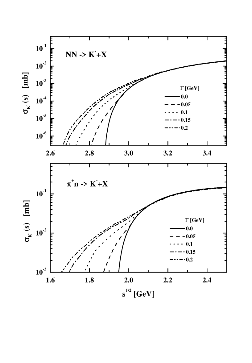
Figure 4: The $K^{-}$ cross section from $NN$ (upper part) and $\pi N$ (lower part) collisions as a function of the invariant energy $\sqrt{s}$ for different collisional width $\Gamma$ of the antikaon spectral function in the medium according to the model discussed in the text.

The resulting cross sections for $K^{-}$ production from $NN$ and $\pi^{+}p$ collisions are displayed in Fig. 4 as a function of $\sqrt{s}$ for different collisional width $\Gamma_{coll}$= 0, 50, 100, 150, 200 MeV while keeping $\sqrt{s_{0}}=M_{K}+M_{N}+M_{\Lambda}$ or $\sqrt{s_{0}}=M_{K}+M_{\Lambda}$, respectively. With increasing width $\Gamma_{coll}$ the subthreshold production of mesons becomes enhanced considerably relative to the respective vacuum cross section, but the absolute magnitude stays small below threshold even for $\Gamma_{coll}$ = 200 MeV.

As a next step we have to fix the collisional width of the hadrons in the nuclear medium which enters the spectral function $A(X,{\vec{P}},M^{2})$ as well as the differential cross sections (43). According to (36) the collisional width is explicitly momentum- (and energy-) dependent. Whereas in Ref. [30] we have employed momentum-independent collisional broadening, this is no longer adequate for relativistic systems. We thus evaluate $\Gamma_{coll}$ for each particle in a finite cell in coordinate space according to (36), however, discard the explicit dependence on the energy $P_{0}$. This approximation implies that the correction factors $(1-C_{(i)})^{-1}$ in the testparticle equations of motion (18) – (20) are equal to 1 and all particles can be propagated with the same system time.

In case of kaons, antikaons or $\rho$ mesons at SIS energies we treat the latter perturbatively as in Ref. [47], i.e. each testparticle achieves a weight $W_{i}$ defined by the ratio of the individual production cross section to the total $\pi B$ or $BB$ cross section at the same invariant energy. Their propagation and interactions are evaluated as for baryons and pions, however, the baryons (pions) are not changed in their final state when interacting with a ’perturbative’ particle. The actual collisional width then is approximated by

$$\Gamma_{coll}^{i}\approx\gamma_{i}\frac{\sum_{j}v_{ij}\sigma_{ij}}{\sum_{j}}\,,$$ (47)

where the sum over $j$ runs over all baryons in the local cell, $v_{ij}$ is the relative velocity in the meson-baryon cms, $\gamma_{i}$ is the Lorentz-factor of the particle with respect to the local rest frame of the baryons and $\sigma_{ij}$ their total cross section at invariant energy $\sqrt{s}_{ij}$. Note, that in (47) the final state Pauli-blocking has been neglected for the baryon which should be reasonable at the high bombarding energies of interest here.

Apart from the description of particle propagation and rescattering the results of the transport approach also depend on the initial conditions, ${\vec{X}}_{i}(0),{\vec{P}}_{i}(0),M_{i}^{2}(0)$. In view of nucleus-nucleus collisions, i.e. two nuclei impinging towards each other with a laboratory momentum per particle $P_{lab}/A$, the nuclei can be considered as in their respective groundstate, which in the semiclassical limit is given by the local Thomas-Fermi distribution [3]. Additionally the virtual mass $M_{i}^{2}$ for nucleons has been determined by Monte-Carlo according to the Breit-Wigner distribution (12) assuming an in-medium width $\Gamma_{0}$ = 1 MeV. We mention that varying $\Gamma_{0}$ from 1 – 5 MeV does not change the results to be presented in Section 3 within the statistics achieved. For the vacuum width of stable hadrons we have used $\Gamma_{V}$ = 1 MeV which implies that nucleons propagating to the continuum in the final state of the reaction achieve their vacuum mass on the 0.1 $\%$ level.

3 Nucleus-nucleus collisions

Our concrete applications we first carry out for nuclear reactions at SIS energies (1 - 2 A GeV) that have been analysed within conventional transport models to a large extent (cf. Ref. [7] and Refs. cited therein).

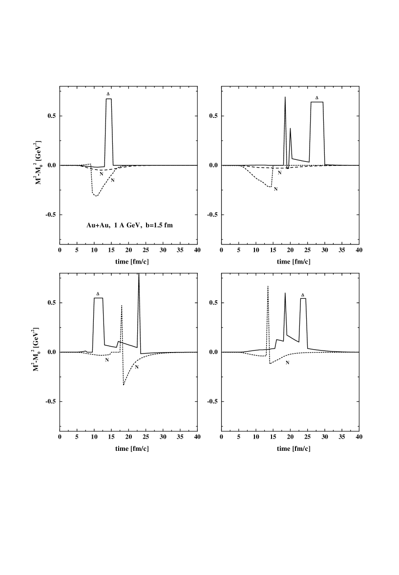
Figure 5: Some randomly chosen examples for the baryon off-shell propagation in mass in $Au+Au$ collisions at 1 A GeV and $b$ = 1.5 fm. The sudden spikes correspond to $\Delta$ or $N^{*}$ excitations.

In view of Eq. (23) we present for some randomly chosen testparticles $i$ the off-mass-shell behaviour $M_{i}^{2}(t)-M_{0}^{2}$ as a function of time in a central collision ($b$ = 1.5 fm) in Fig. 5 for $Au+Au$ at 1 A GeV. It is seen that during the collision of the nuclei from $t\approx$ 7 – 25 fm/c the off-shellness of baryons reaches up to 0.8 GeV², however, the nucleons become practically on-shell for $t\geq$ 35 fm/c. The individual sudden high mass excitations and subsequent decays correspond essentially to $\Delta$ and N(1440) baryons. Nucleons in their decay may be off-shell, but propagate again to their on-shell mass in the continuum.

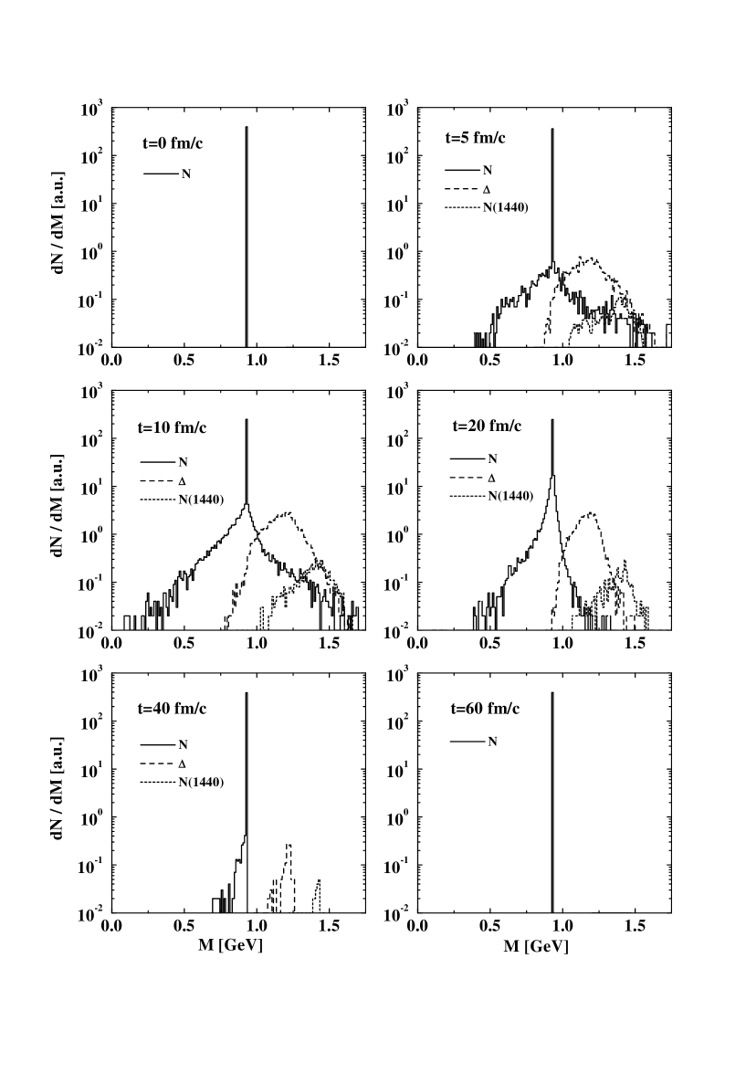
Figure 6: The baryon distribution in mass $M$ for $Au+Au$ at 1 A GeV and $b$ = 1.5 fm for times of 0, 5, 10, 20, 40 and 60 fm/c. The dashed and dotted lines stand for $\Delta$ and $N(1440)$ resonances, respectively.

The baryon spectral function is shown in Fig. 6 as a function of the invariant mass for the latter reaction at times of 0, 5, 10, 20, 40 and 60 fm/c. Apart from a broadening of the nucleon spectral function at the initial time steps one observes that the high mass tail is completely covered by the $\Delta$ and N(1440) excitations. This is different from the results in [30] at GANIL energies since in the latter case the $\Delta$ excitation was dynamically suppressed and the high mass tail of the spectral function dominated by nucleons. In fact, in 1 A GeV $Au+Au$ collisions the resonance high mass spectrum in the off-shell calculations is only slightly enhanced as compared to the on-shell calculations (without explicit representation). Note that at t = 60 fm/c all resonances have decayed and the nucleons have become on-shell again.

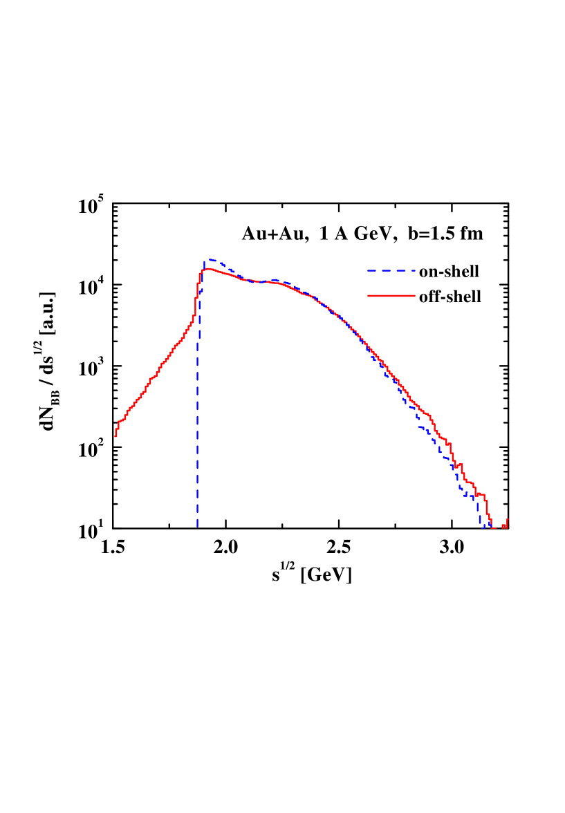
Figure 7: The number of baryon-baryon (BB) collisions as a function of the invariant energy $\sqrt{s}$ for $Au+Au$ at 1 A GeV and $b$ = 1.5 fm. The solid line is obtained from including the off-shell propagation of baryons in the transport approach while the dashed line stands for the result in the on-shell limit.

The dominance of the resonances for the high mass tail can also be seen in the differential collision number $dN_{coll}/d\sqrt{s}$ for baryon-baryon collisions which is displayed in Fig. 7. Here the dashed histogram stands for the on-shell result while the solid histogram gives the off-shell distribution that extends well below the two-nucleon threshold. The high energy tail in this distribution dominantly arises from $N\Delta$ and $\Delta\Delta$ or $NN(1440)$ reactions, which are similar in both calculations. We thus find only a small enhancement in the high energy tail for the off-shell case relative to the on-shell limit.

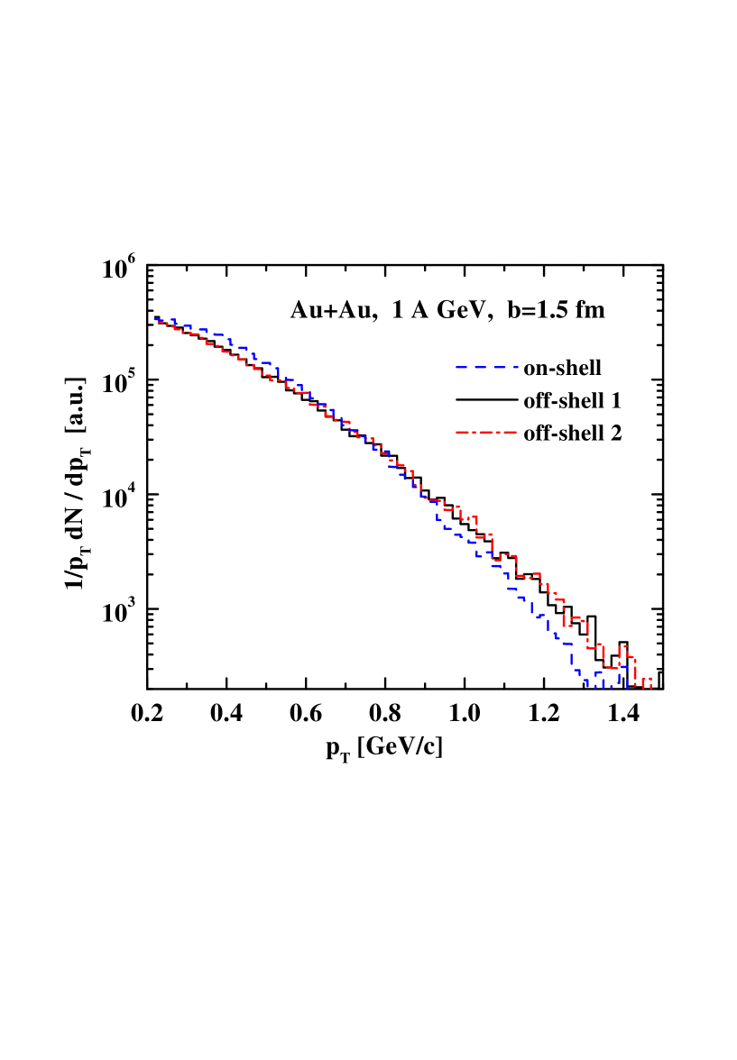
Figure 8: The transverse momentum spectra of protons $1/p_{T}dN_{p}/dp_{T}$ for $Au+Au$ at 1 A GeV and impact parameter $b$ = 1.5 fm. The dashed histogram is the result from the on-shell propagation while the solid histogram is obtained including the ’default’ off-shell propagation of baryons. The dot-dashed histogram displays the result for an alternative modelling of the ’off-shell’ elastic $NN$ collisions (see text); the two off-shell calculations give the same $p_{T}$ spectra within the statistical accuracy.

The latter observation can also be made in the transverse proton momentum spectra $1/p_{T}dN_{p}/dp_{T}$ (Fig. 8) for $Au+Au$ at 1 A GeV ($b$=1.5 fm) where the on-shell propagation (dashed histogram) practically leads to the same result as the off-shell propagation (solid histogram) except for the high momentum tail. Since the elastic $NN$ cross section is taken here as a function of the momentum difference in the cms (cf. Section 2.4) one might worry if alternative prescriptions for $\sigma_{NN}$ could change the results. In this context we have performed calculations using the Cugnon parametrization $\sigma_{NN}(\sqrt{s})$ with $\sqrt{s}$ denoting the actual invariant energy of the off-shell nucleons and adopting $\sigma_{NN}$ = 55 mb for invariant energies below 2 $m_{N}$, where $m_{N}$ denotes the nucleon vacuum mass. The transverse momentum spectra according to this recipe (for the same reaction) are shown in Fig. 8 in terms of the dot-dashed histogram, which coincides with the ’default’ off-shell result (solid histogram) within the statistics.

3.1 Meson production at SIS energies

In principle also the pions should be propagated with a dynamical spectral function since their coupling to nucleons is very strong. In fact, pion collision rates in these reactions lead to a collisional width which is much larger than the pion mass itself. A straight forward selection of pion masses (e.g. in the $\Delta$ decay) according to such a dynamical spectral function leads to $M_{\pi}^{2}<0$ which implies that such testparticles become acausal, i.e. move with velocities $\beta>$ 1. In order to avoid such inconsistencies we treat pions on-shell throughout this study. We note, however, that microcausality is an essential issue that should also survive in transport approximations. This is practically done by the explicit requirement $M^{2}_{i}\geq 0$ in the transport calculation, but not yet inherent in eqs. (18-20).

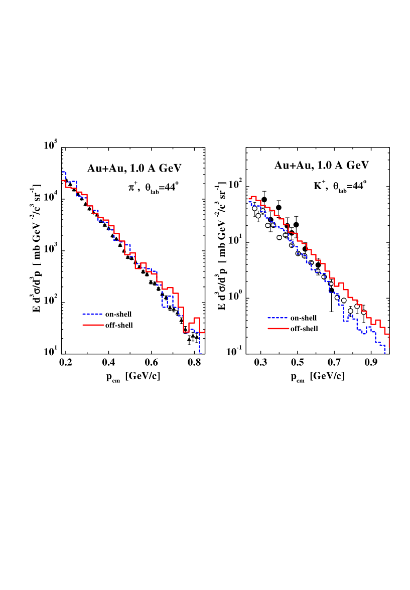
Figure 9: (l.h.s.): The inclusive momentum spectra of positive pions at $\theta_{lab}=44\pm 4^{o}$ for $Au+Au$ at 1 A GeV in comparison to the experimental data from the KaoS Collaboration [40] (full triangles) displayed as a function of the momentum in the nucleus-nucleus cms. (r.h.s.): The inclusive momentum spectra of positive kaons at $\theta_{lab}=44\pm 4^{o}$ for $Au+Au$ at 1 A GeV in comparison to the experimental data from the KaoS Collaboration (full circles [41], open circles [42]). The dashed histograms show the results from the on-shell propagation while the solid histograms are obtained including the off-shell propagation of baryons. The fluctuations of the histograms with respect to an average exponential spectrum provide an estimate for the statistical error bars of the calculations.

Since the authors of Ref. [31] claim a large enhancement in the pion yield for $Au+Au$ at 1 A GeV and especially in the high energy tails of the pion spectrum when describing nucleon off-shell propagation in their Monte-Carlo simulation, we show in Fig. 9 (l.h.s.) the inclusive differential $\pi^{+}$ spectrum for this system at $\theta_{lab}=44\pm 4^{o}$ within our off-shell approach (solid histogram) in comparison to the on-shell limit (dashed histogram) and the experimental data from the KaoS collaboration [40]. As in Ref. [44] the $\pi^{+}$ spectrum is described quite well within the on-shell HSD approach. As also seen from Fig. 9 there is only a very slight enhancement of the high momentum tail in the pion spectrum for our off-shell calculation which is still compatible with the experimental spectrum from Ref. [40] within the statistical errors. Note that the fluctuations in the histograms with respect to an average exponential spectrum provide some information about the statistical accuracy. Thus our off-shell approach – based on the Kadanoff-Baym equation (16) – is not in conflict with the experimental data contrary to the model from Ref. [31].

Since kaons couple only weakly to nucleons and are not absorbed at low energies their collisional width is rather small such that they may be treated on-shell to a good approximation. In their differential production cross section we thus only can test the effects from the off-shell propagation of baryons. The inclusive $K^{+}$ spectra at $\theta_{lab}=44\pm 4^{o}$ for $Au+Au$ at 1 A GeV are shown in Fig. 9 (r.h.s.) where we compare our off-shell results (solid histogram) with the on-shell limit (dashed histogram) and the experimental data from Ref. [41] (full circles) and Refs. [42, 43] (open circles) where the latter differ on average by a factor of 2. The off-shell calculations give a slightly higher $K^{+}$ yield than the on-shell calculations, however, are still well within the error bars of the presently available data. We mention that we have performed the calculations without any kaon potential; a slightly repulsive kaon potential will drop the $K^{+}$ yield and harden the spectrum slightly as discussed in Ref. [44].

The relative increase of the $K^{+}$ spectrum by about 50% in the off-shell calculation with respect to the on-shell result should also be compared with the relative sensitivity to the incompressibility $K$ of the nuclear equation-of-state (EoS) [45]. According to the early relativistic calculations by Lang et al. [46] the inclusive $K^{+}$ yield in $Au+Au$ collisions at 1 A GeV is enhanced by about a factor of 2 when decreasing the incompressibility $K$ from 380 MeV to 200 MeV. When restricting to incompressibilities 200 MeV $\leq K\leq$ 300 MeV this relative sensitivity reduces to a similar change in the $K^{+}$ yield for $Au+Au$ at 1 A GeV as obtained from the off-shell dynamics relative to the on-shell treatment. It thus appears questionable if the incompressibility of the EoS can be determined from the systematics of $K^{+}$ spectra alone since also the $K^{+}$ in-medium potential potential is not yet determined very accurately.

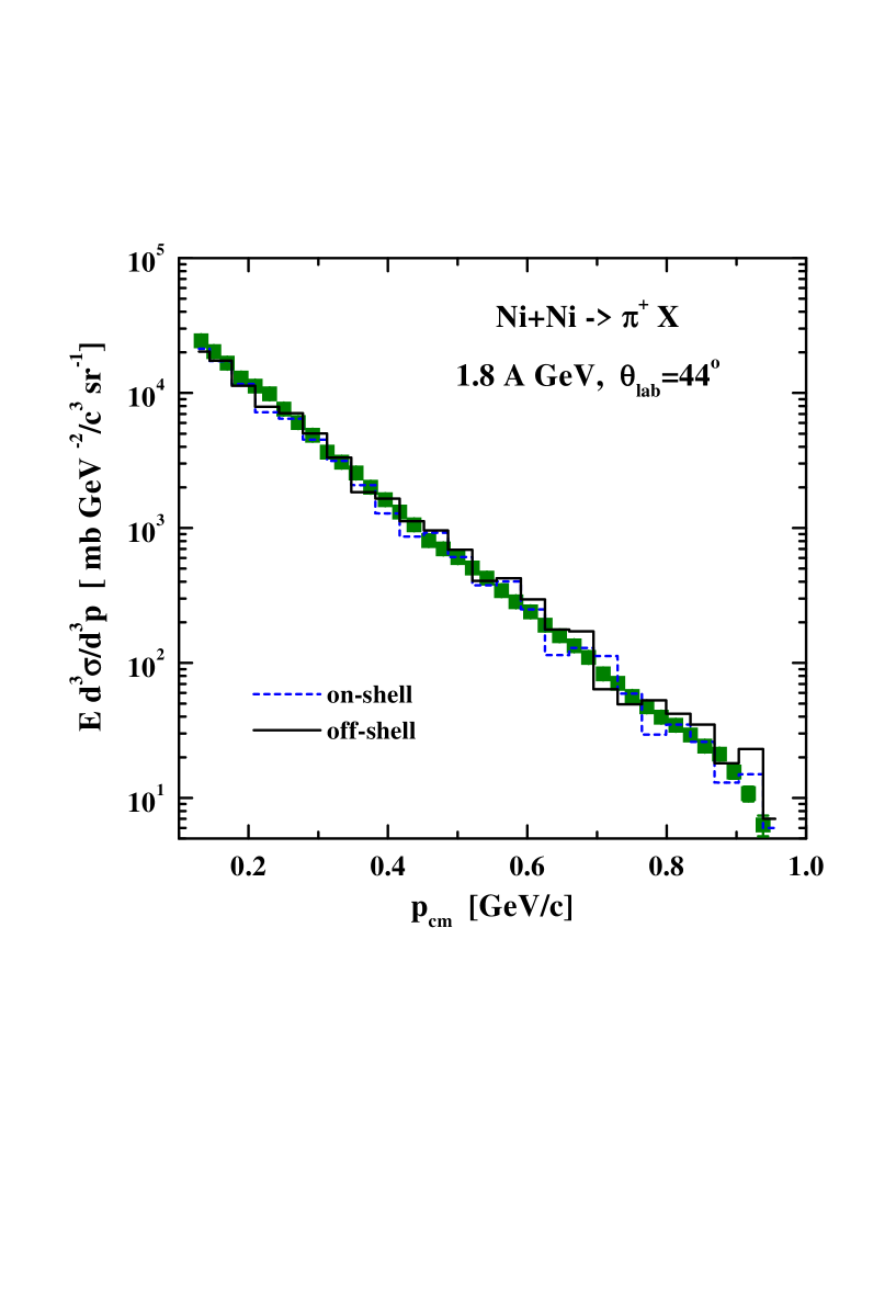
Figure 10: The inclusive spectra of positive pions for $Ni+Ni$ at 1.8 A GeV including the off-shell propagation in the transport approach (solid histogram) and in the on-shell limit (dashed histogram) in comparison to the experimental data from [43] (full squares) at $\theta_{lab}$ = 44^o.

We continue with pion production in $Ni+Ni$ collisions at 1.8 A GeV since for this system also $K^{+}$ and $K^{-}$ spectra have been measured [42, 40, 43]. The inclusive differential cross section for $\pi^{+}$ from $Ni+Ni$ collisions at 1.8 A GeV is shown in Fig. 10 as a function of the pion momentum in the cms in comparison to the data of the KaoS Collaboration taken at $\Theta_{lab}=44\pm 4^{0}$ [42, 43]. The calculation with an off-shell propagation of baryons is represented by the solid histogram while the on-shell limit is displayed in terms of the dashed histogram. Within the numerical accuracy both results almost coincide which in view of Fig. 7 is not an exciting surprise. Both results, furthermore, are in a reasonable agreement with the measured spectrum (full squares) which suggests that no ’unphysical’ approximations have been introduced within the ’recipies’ for the off-shell transition cross sections.

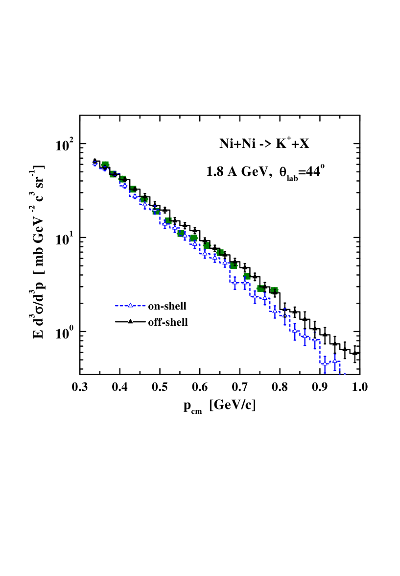
Figure 11: The inclusive spectra of positive kaons for $Ni+Ni$ at 1.8 A GeV including the off-shell propagation in the transport approach (solid histogram, full triangles) and in the on-shell limit (dashed histogram, open triangles) in comparison to the experimental data from [43] (full squares) at $\theta_{lab}$ = 44^o. The ’theoretical’ error bars are statistical, only (see text).

As might have been anticipated from the studies before, also the inclusive $K^{+}$ spectra from $Ni+Ni$ at 1.8 A GeV – plotted as a function of the kaon momentum in the cms – is only weakly sensitive to the off-shell propagation of baryons as shown in Fig. 11 since the differential $\sqrt{s}$ distribution for baryon-baryon collisions does not differ very much and also the pion-baryon production channel is similar (except for the high momentum tail). The latter fact one might also extract from the low sensitivity of the pion spectrum to an off-shell propagation in Fig. 10 for this reaction. We note that the kaons again have been propagated without any in-medium potential, which should be slightly repulsive in line with Refs. [49, 50, 51]. As shown in Ref. [44] such a repulsive potential will suppress the kaon spectra especially at low momenta. Since we have employed the same production cross sections as in Ref. [44] we again reproduce the data from the KaoS Collaboration, taken at $\Theta_{lab}=44\pm 4^{0}$, best without a kaon potential, where the off-shell calculation seems to be in even better agreement with the data. We mention that the ’theoretical’ error bars in Fig. 11 are of statistical nature only and computed as $\pm 0.5S_{p}/\sqrt{N_{p}}$ where $S_{p}$ is the calculated spectral point in the actual momentum bin and $N_{p}$ denotes the number of events contributing to this momentum bin. Though the error bars between the on-shell (open triangles) and off-shell calculation (full triangles) almost overlap, we point out that the off-shell calculation gives a slightly harder spectrum.

Note that the production channel $N\Delta\rightarrow NK^{+}Y$, where $Y$ denotes a hyperon, as well as the $\Delta\Delta\rightarrow K^{+}NY$ channel is not known experimentally and simple isospin factors as extracted from pion exchange [44] might not be appropriate. Though there are some recent efforts to resolve this uncertainty within extended boson exchange models [55], the latter models will hardly be tested experimentally. This general uncertainty has to be kept in mind when comparing transport calculations to experimental kaon spectra.

We step on with the production of antikaons in the same reaction. Antikaons couple strongly to nucleons and thus achieve a large collisional width in the nuclear medium. The calculations of Ref. [52], which are based on a dispersion approach, give a collisional width of about 100 MeV of $K^{-}$ mesons at moderate momenta and nuclear matter density $\rho_{0}$. Thus off-shell antikaons might be produced at far subthreshold energies (cf. Fig. 4), become asymptotically on-shell and thus enhance the $K^{-}$ yield. Note, that this mechanism also might explain the $K^{-}$ enhancement seen by the FRS, KaoS and FOPI collaborations [43, 48, 53] in $Ni+Ni$ reactions around 1.8 A GeV.

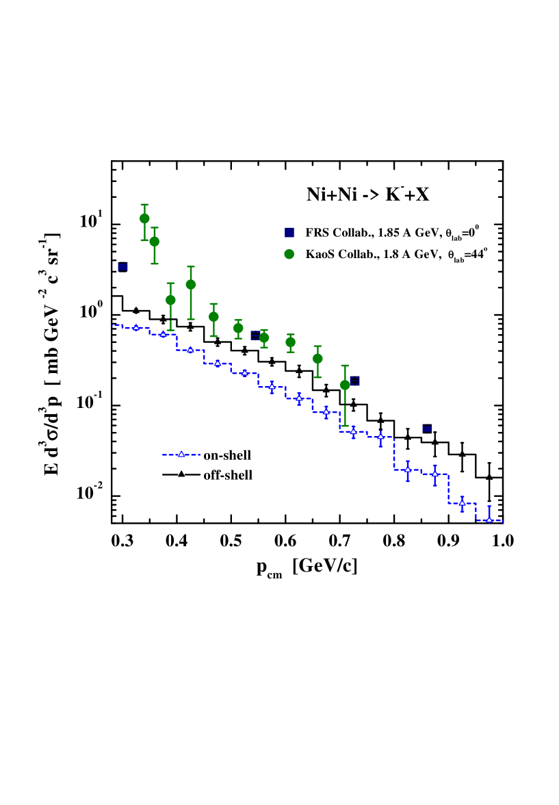
Figure 12: The inclusive spectra of $K^{-}$ for $Ni+Ni$ at 1.8 A GeV including the off-shell propagation in the transport approach (solid histogram, full triangles) and in the on-shell limit (dashed histogram, open triangles) in comparison to the experimental data from Refs. [43] (open circles) and [53] (full squares) at $\theta_{lab}$ = 44^o and $\theta_{lab}$ = 0⁰, respectively. Note that no antikaon potentials have been included in the calculations. The ’theoretical’ error bars are statistical, only (see text).

Within our present ’modelling’ of off-shell production processes, which are governed by phase-space close to threshold energies, we find an enhancement by about a factor $\sim$ 2 in the production of antikaons when treating baryons as well as antikaons off-shell. This is demonstrated in Fig. 12 where we show the $K^{-}$ spectra as a function of their momentum in the cms for the off-shell (solid histogram, full triangles) and on-shell propagation (dashed histogram, open triangles). As in case of Fig. 11 the ’theoretical’ error bars are statistical, only, and taken as $\pm 0.5S_{p}/\sqrt{N_{p}}$ where $S_{p}$ and $N_{p}$ denote the actual value in the momentum bin and number of events, respectively. Both results underestimate the data from the FRS and KaoS Collaborations [42, 43, 53] such that the conclusion in Refs. [47, 54] on attractive $K^{-}$ self energies in the nuclear medium persists, though the off-shell calculations suggest somewhat smaller $K^{-}$ potentials. We mention that the dispersion analysis of the $K^{-}$ potential in nuclear matter in Ref. [52] also yields somewhat smaller antikaon potentials than that extracted in Refs. [47, 54] which is in line with our present finding. However, in order to obtain more model independent results on the antikaon self energy, precise data on antikaon flow from nucleus-nucleus collisions are urgently needed.

3.2 AGS energies

At AGS energies of $\approx$ 11 A GeV the invariant energy $\sqrt{s}$ of the initial nucleon-nucleon collisions is about 5 GeV which implies that the nucleons are excited to continuum states – denoted by strings – which decay according to phase-space [56] and fixed quark/diquark or $s/(u,d)$ ratios after a formation time $\tau_{F}$ = 0.8 fm/c. Some details of the decay scheme are given in Ref. [57]. The FRITIOF 7.2 version - as implemented in the HSD transport approach - also includes the production of unstable particles of width $\Gamma_{h}$ by Monte-Carlo. The width $\Gamma_{h}$ has been modified dynamically according to the actual total width at space-time point $X$ which allows to simulate the production of hadrons with broad spectral functions from string decay in a straight forward manner. The low energy baryon-baryon and meson-baryon reactions are treated as for SIS energies (cf. Section 2.4).

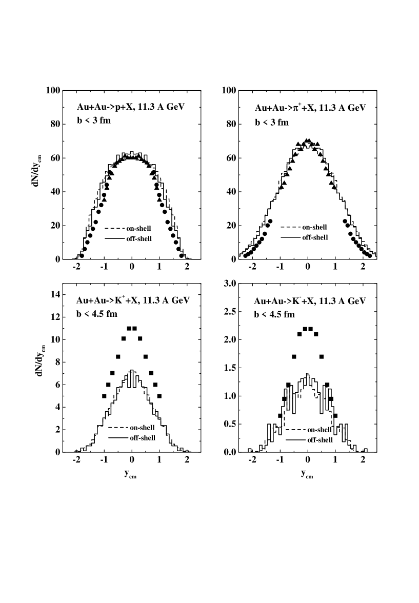
Figure 13: The rapidity distributions of protons, $\pi^{+},K^{+}$ and $K^{-}$ for central collisions of $Au+Au$ at 11.3 A GeV in comparison to the data from Refs. [58, 59]. The solid histograms are obtained including the off-shell propagation in the transport approach while the dashed histograms result from the on-shell limit.

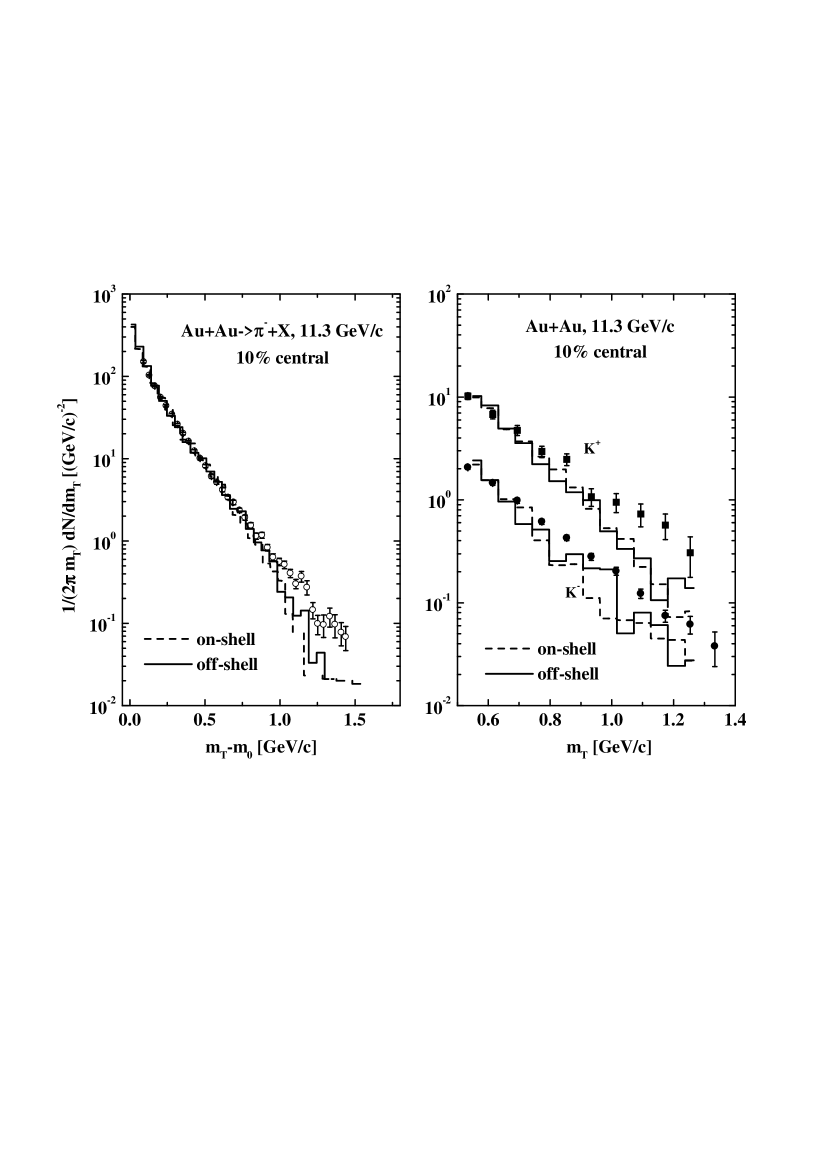
Figure 14: The transverse mass spectra of $\pi^{+}$ (l.h.s.), $K^{+}$ and $K^{-}$ mesons (r.h.s.) for central collisions of $Au+Au$ at 11.3 A GeV in comparison to the data from Refs. [59]. The solid histograms are obtained including the off-shell propagation in the transport approach while the dashed histograms result from the on-shell limit.

We here present only a single study for central $Au+Au$ reactions at 11.3 A GeV ($b\leq$ 3.5 fm) and concentrate on the rapidity and transverse mass spectra of pions, kaons and antikaons. The results of our calculations are displayed in Figs. 13 and 14 for the off-shell calculation (solid histograms) and the on-shell calculations (dashed histograms) in comparison to the data from Refs. [58, 59]. Since at this bombarding energy the dynamics are dominated by continuum string excitations, a broadening of the spectral functions is found to play a minor role here. Note, that the $K^{\pm}$ spectra for $Au+Au$ collisions at AGS energies are underestimated in comparison to the data, which in Ref. [57] has been attributed to nonhadronic degrees of freedom or a partial restoration of chiral symmetry during the high density collision phase.

4 Summary

In this work we have employed the semiclassical off-shell transport approach from Ref. [30], that in first order in the gradient expansion describes the virtual propagation of particles in the invariant mass squared $M^{2}$ besides the conventional propagation in the mean-field potential (given by the real part of the retarded self energy), to analyse nucleus-nucleus collisions at SIS and AGS energies. Note that in conventional transport approaches the imaginary part of the self energy is reformulated in terms of a collision integral and simulated by on-shell binary collisions, only. We here additionally account for the off-shell propagation of particles due to the imaginary part of the self energy in eqs. (18,19,23) which describe the dynamical evolution of the particle spectral function. The additional imaginary part of the self energy (or local collision rate $\Gamma_{coll}$) is determined by the collision integrals themselves and can be used in transport approaches without introducing any new assumptions or parameters provided that the off-shell transition amplitudes $T$ are known in the collision integral (26). In addition to Ref. [30] we have included momentum-dependent self energies for baryons and mesons in our present approach. However, a final answer to the role of off-shell hadrons in nucleus-nucleus collisions we still have to leave for future due to the ’ad hoc’ assumptions involved in the treatment of the off-shell transition probabilities.

We have presented dynamical calculations of the novel transport theory for nucleus-nucleus collisions at SIS and AGS energies where we can test its results in comparison to experimental data. We find that the off-shell propagation of nucleons practically does not change the rapidity distributions $dN/dy$ and has only a minor effect on the transverse momentum spectra of protons within the statistics reached except for the very high momentum tails. The distribution of baryon-baryon collisions in the invariant energy $\sqrt{s}$ is found to be also enhanced only for high invariant energies since here the collisions with or between resonances – which are only slightly affected in their high mass spectrum – dominate the spectrum. Again except for high momentum tails we find no dramatic change in the pion and $K^{+}$ spectra at SIS energies for $Au+Au$ at 1.0 A GeV and $Ni+Ni$ at 1.8 A GeV, our results being well in line with the data of the KaoS Collaboration. This no longer holds for the $K^{-}$ spectra from $Ni+Ni$ collisions at 1.8 A GeV which are enhanced by a factor of $\sim$ 2 relative to the on-shell calculation within the statistics reached. We attribute this enhancement to a broad spectral function of antikaons at high baryon density and to the ’subthreshold’ energy of 1.8 A GeV considered. However, even in case of the off-shell propagation of baryons and mesons the experimental $K^{-}$ spectra are underestimated and attractive antikaon potentials are still needed to achieve a proper description.

At AGS energies ($\approx$ 11 A GeV) the particle production in the HSD approach essentially occurs via the excitation and decay of strings which can be viewed as continuum excitations of hadrons. Any spectral broadening of the ’continuum’ thus is not likely to be seen in the asymptotic particle spectra of pions, kaons or antikaons especially since they are most abundantly produced far above the individual $NN$ or $\pi N$ thresholds.

We finally point out that although our off-shell transport approach appears to be in a reasonable agreement with the differential experimental data at least for SIS energies (except for $K^{-}$ when discarding antikaon potentials), the question of proper off-shell transition amplitudes in the collision terms remains an open problem that has to addressed in the near future. Some steps in this direction e.g. have been taken in Ref. [60].

The authors like thank E. L. Bratkovskaya, C. Greiner and S. Leupold for stimulating discussions throughout this study. Furthermore, they also acknowledge lively, though controversal, exchange of arguments with M. Effenberger and U. Mosel.

a

a

a

a

a

a

a

a

a

a

a

a

a

a

References

- [1] H. Stöcker and W. Greiner, Phys. Rep. 137 (1986) 277.
- [2] G. F. Bertsch and S. Das Gupta, Phys. Rep. 160 (1988) 189.
- [3] W. Cassing, V. Metag, U. Mosel and K. Niita, Phys. Rep. 188 (1990) 363.
- [4] W. Cassing and U. Mosel, Prog. Part. Nucl. Phys. 25 (1990) 235.
- [5] A. Faessler, Prog. Part. Nucl. Phys. 30 (1993) 229.
- [6] S. Bass et al., Prog. Part. Nucl. Phys. 41 (1998) 255; J. Phys. G 25 (1999) R1.
- [7] W. Cassing and E. L. Bratkovskaya, Phys. Rep. 308 (1999) 65.
- [8] L. P. Kadanoff and G. Baym, Quantum statistical mechanics, Benjamin, New York, 1962.
- [9] P. Danielewicz, Ann. Phys. (N.Y.) 152 (1984) 239; ibid. 305.
- [10] W. Botermans and R. Malfliet, Phys. Rep. 198 (1990) 115.
- [11] R. Malfliet, Prog. Part. Nucl. Phys. 21 (1988) 207.
- [12] P. A. Henning, Nucl. Phys. A 582 (1995) 633; Phys. Rep. 253 (1995) 235.
- [13] C. Greiner and S. Leupold, Ann. Phys. (N.Y.) 270 (1998) 328.
- [14] S. J. Wang and W. Cassing, Ann. Phys. (N.Y.) 159 (1985) 328.
- [15] S. J. Wang, W. Zuo and W. Cassing, Nucl. Phys. A 573 (1994) 245.
- [16] W. Cassing and S. J. Wang, Z. Phys. A 337 (1990) 1.
- [17] W. Cassing, K. Niita and S. J. Wang, Z. Phys. A 331 (1988) 439.
- [18] J. Knoll, Prog. Part. Nucl. Phys. 42 (1999) 177.
- [19] Yu. B. Ivanov, J. Knoll, and D. N. Voskresensky, nucl-th/9905028.
- [20] C. M. Ko and G. Q. Li, J. Phys. G: Nucl. Part. Phys. 22 (1996) 1673.
- [21] K. Niita, W. Cassing and U. Mosel, Nucl. Phys. A 504 (1989) 391.
- [22] Gy. Wolf, G. Batko, W. Cassing, U. Mosel, K. Niita and M. Schäfer, Nucl. Phys. A 517 (1990) 615.
- [23] J. Aichelin, Phys. Rep. 202 (1991) 233.
- [24] S. W. Huang, A. Faessler, G. Q. Li, D. T. Khoa, E. Lehmann, R. K. Puri, M. A. Matin, and N. Ohtsuka, Prog. Part. Nucl. Phys. 30 (1993) 105.
- [25] G. Q. Li, A. Faessler and S. W. Huang, Prog. Part. Nucl. Phys. 30 (1993) 159.
- [26] T. Maruyama, W. Cassing, U. Mosel, S. Teis and K. Weber, Nucl. Phys. A 573 (1994) 653.
- [27] B. A. Li and C. M. Ko, Phys. Rev. C 52 (1995) 2037.
- [28] S. H. Kahana, D. E. Kahana, Y. Pang and T. J. Schlagel, Annu. Rev. Nucl. Part. Sci. 46 (1996) 31.
- [29] W. Ehehalt and W. Cassing, Nucl. Phys. A 602 (1996) 449.
- [30] W. Cassing and S. Juchem, nucl-th/9903070, Nucl. Phys. A (2000), in press.
- [31] M. Effenberger and U. Mosel, nucl-th/9906085, Phys. Rev. C 60 (1999) 51901.
- [32] T. Kodama, S.B. Duarte, K.C. Chung, R. Donangelo and R.A.M.S. Nazareth, Phys. Rev. C 29 (1984) 2146.
- [33] J. Cugnon, D. Kinet and J. Vandermeulen, Nucl. Phys. A 379 (1982) 553.
- [34] E. Bycking and K. Kajantie, Particle Kinematics, John Wiley and Sons, 1973.
- [35] S. Teis et al., Z. Phys. A 356 (1997) 421.
- [36] M. Effenberger, E. L. Bratkovskaya and U. Mosel, nucl-th/9903026, Phys. Rev. C 60 (1999) 44614.
- [37] N. Bianchi et al., Phys Rev. C 54 (1996) 1688.
- [38] S. Teis et al., Phys. Rev. C50 (1994) 388.
- [39] A. Sibirtsev, W. Cassing, G. I. Lykasov, and M. V. Rzjanin, Nucl. Phys. A 632 (1998) 131.
- [40] C. Müntz et al., Z. Phys. A 352 (1995) 17; D. Brill et al., Z. Phys. A 357 (1997) 207.
- [41] D. Miskowiec et al., Phys. Rev. Lett. 72 (1994) 3650.
- [42] P. Senger and the KaoS Collaboration, in ’Heavy Ion Physics at Low, Intermediate and Relativistic Energies Using Detectors’, ed. by M. Petrovici et al., World Scientific 1997, p. 313.
- [43] P. Senger for the KaoS Collaboration, Acta Physica Polonica B 27 (1996) 2993.
- [44] E. L. Bratkovskaya, W. Cassing and U. Mosel, Nucl. Phys. A 622 (1997) 593.
- [45] J. Aichelin and C. M. Ko, Phys. Rev. Lett. 55 (1985) 2661.
- [46] A. Lang, W. Cassing, U. Mosel, and K. Weber, Nucl. Phys. A 541 (1992) 507.
- [47] W. Cassing, E.L. Bratkovskaya et al., Nucl. Phys. A 614 (1997) 415.
- [48] F. Laue et al., Phys. Rev. Lett. 82 (1999) 1640.
- [49] D. B. Kaplan and A. E. Nelson, Phys. Lett. B 175 (1986) 57.
- [50] T. Waas, N. Kaiser and W. Weise, Phys. Lett. B 379 (1996) 34.
- [51] J. Schaffner-Bielich, I. N. Mishustin and J. Bondorf, Nucl. Phys. A 625 (1997) 325.
- [52] A. Sibirtsev and W. Cassing, Nucl. Phys. A 641 (1998) 476.
- [53] A. Schröter et al., Z. Phys. A 350 (1994) 101.
- [54] G. Q. Li, C.-H. Lee and G. E. Brown, Nucl. Phys. A 625 (1997) 372.
- [55] K. Tsushima et al., Phys. Rev. C 59 (1999) 369.
- [56] B. Anderson, G. Gustafson and Hong Pi, Z. Phys. C 57 (1993) 485.
- [57] J. Geiss, W. Cassing and C. Greiner, Nucl. Phys. A 644 (1998) 107.
- [58] R. Ganz et al., J. Phys. G 25 (1999) 247; C. A. Ogilvie, J. Phys. G 25 (1999) 159.
- [59] C. A. Ogilvie for the E866 and E819 Collaborations, Nucl. Phys. A 638 (1998) 57c; L. Ahle et al., Nucl. Phys. A 610 (1996) 139c; L. Ahle et al., Phys. Rev. C 57 (1998) R466; Phys. Rev. C 60 (1999) 044904.
- [60] P. Bozek, nucl-th/9910022.
- [61] S. Leupold, nucl-th/9909080.