Perturbative Effective Field Theory at Finite Density

Abstract

An accurate description of nuclear matter starting from free-space nuclear forces has been an elusive goal. The complexity of the system makes approximations inevitable, so the challenge is to find a consistent truncation scheme with controlled errors. Nonperturbative effective field theories could be well suited for the task. Perturbative matching in a model calculation is used to explore some of the issues encountered in extending effective field theory techniques to many-body calculations.

I Introduction

Nuclear forces have been studied in depth over the past fifty years, leading to excellent phenomenological descriptions [1]. A main goal of this enterprise has been to arrive at the “best” two-nucleon potential and to use it in many-body calculations to determine the properties of nuclear matter and finite nuclei. Effective field theory (EFT) analyses [2] offer a different perspective: There is no best two-body potential. Indeed, the off-shell behavior of a potential or amplitude is not observable and should not influence the predictability of the theory if a consistent power-counting scheme is used [3]. In addition, many-body contact terms are an inevitable consequence of using low-energy degrees of freedom and so must be included along with two-body interactions to eliminate off-shell ambiguities [4, 5]. Finally, the symmetries of the underlying theory of QCD can be used to constrain the interactions, such as using chiral symmetry to describe two-pion exchange [6, 7]. These features merit a reanalysis of nuclear matter within the context of an EFT.

Effective field theory techniques may also offer special advantages for many-body systems, where exact solutions are not realizable. Estimates of the errors in approximate calculations and clear guidelines for making systematic improvements are hallmarks of an EFT. Even with a well-behaved underlying theory, like QED, an EFT can be beneficial for organizing the contributions from various effects, as NRQED does for the radiative corrections to positronium [8]. Similar benefits may result from an application of EFT to nuclear matter.

Skyrme wrote down the first effective theory for nuclear matter [9] and used properties of nuclei to fit parameters in a mean-field lagrangian. Early attempts to motivate these parameters from the free-space nucleon-nucleon potential were promising [10], but were shown to depend on the form of the two-body potential [11]. More recent studies have focused on scaling properties near the Fermi surface [12, 13, 14] to determine which operators are important for Fermi liquids [15] as well as to describe the pairing gap [16]. The behavior of nuclear binding in the chiral limit [17] and the nature of the bound state in nuclear matter [18] were also examined recently, but without a connection to free-space parameters. Here we focus on the use of an effective lagrangian with parameters fit from free-space and few-body data.

The effective lagrangian consists of long-range interactions constrained by chiral symmetry and the most general short-range interactions consistent with QCD symmetries. The coefficients of these short-range terms may eventually be derived from QCD, but at present must be fit by matching calculated and experimental observables in a momentum expansion. In free space, this expansion is in the external momentum over some breakdown scale $\Lambda$.

For NN scattering, an EFT that consists only of short-range interactions is equivalent to the effective range expansion, which breaks down around $\Lambda\approx m_{\pi}/2$. Using chiral symmetry to explicitly include pions in the lagrangian pushes this scale up to at least $300$ MeV [19, 20, 21], but it may be as high as the $\rho(770)$ mass [22, 23, 24]. This effective lagrangian can then be used to systematically predict other observables, including inelastic processes, up to the same scale. In the following, we discuss extending this procedure to nuclear matter.

If the in-medium expansion parameter is simply the Fermi momentum $k_{F}$ over the free-space breakdown scale $\Lambda$, then $\Lambda\approx 300$ MeV implies that a useful EFT description of equilibrium nuclear matter (where $k_{F}\approx 260$ MeV) might be impossible. The analysis of phenomenologically successful mean-field descriptions of nuclei from an EFT perspective reveals a systematic density expansion, with a characteristic mass scale around $600$ MeV [25, 26]. This suggests that a useful EFT expansion of nuclear matter is plausible if the free-space breakdown scale can be pushed as large as $m_{\rho}$, but a determination of how this expansion carries over to many-body systems is also required.

Important questions about how to do power counting in a fully nonperturbative many-body calculation are as yet unresolved. Nevertheless, we can try to isolate some of the issues and techniques from free-space EFT analyses to explore how they translate to a many-body system. Our strategy here is to extend to the medium the perturbative matching example used by Lepage to illustrate EFT renormalization for ordinary two-body scattering [19]. This enables us to explore the convergence of non-scattering observables, the effective in-medium expansion parameter and breakdown scale, the use of error plots, and regularization dependence. Special considerations required due to the large scattering lengths characteristic of nuclear scattering are postponed to future studies.

The convergence properties of an EFT in the medium can be cleanly tested by fitting to pseudo-data generated from an exact underlying potential that features a characteristic mass scale. A full EFT calculation must include long-range pion effects, but these do not modify the basic analysis presented here, so the role of the pion is ignored in order to keep the discussion as transparent as possible. Similarly, we omit higher partial waves, spin dependence, and relativistic corrections. For our discussion, the only key feature at finite density is the Pauli-blocking of occupied intermediate states. With a simple interaction between nucleons that is perturbative in the coupling, expansion parameters in free space and in the medium can be identified both analytically and using the corresponding error plots.

In Sect. II we perform perturbative matching calculations in free space using a simple model potential, with both dimensional regularization and a cutoff regularization. We illustrate the matching procedure in some detail, as it is likely to be unfamiliar to practitioners of conventional nuclear physics. In Sect. III we apply the EFT to finite density and show how the errors and breakdown scale extend to the medium. The implications for EFT calculations of nuclear matter are discussed in Sect. IV.

II Matching in Free Space

Galilean invariance requires the interaction between two free nucleons of momentum ${\bf k_{1}}$ and ${\bf k_{2}}$ to be independent of their center-of-mass momentum ${\bf P}={\bf k_{1}}+{\bf k_{2}}$. For clarity, we take the underlying potential to be a separable potential in the ${}^{1}\!S_{0}$ -channel that falls off at large momenta and depends on the relative momentum $k\equiv|{\bf k}|\equiv\frac{1}{2}|{\bf k_{1}}-{\bf k_{2}}|$ only,

$$\langle{\bf k^{\prime}}|\hat{V}_{\rm true}|{\bf k}\rangle=\frac{4\pi}{M}\frac{\alpha m^{3}}{(k^{2}+m^{2})(k^{\prime}{}^{2}+m^{2})}\ .$$ (1)

The mass $m$ corresponds to the range (and non-locality) of the potential; it plays the role of the underlying short-distance scale. We adopt an overall normalization of $4\pi/M$, with $M$ the nucleon mass. The dimensionless coupling $\alpha$ provides a perturbative expansion parameter. If $\alpha$ is ${\cal O}(1)$, then the effective range parameters are of “natural” size, which means a constant of order one times, in this case, a power of $m$ (see Appendix A).

An EFT can describe observables from the interaction in Eq. (1) to any desired accuracy as long as the details of the underlying potential are not probed. For scattering observables, this restricts the external momentum $k$ to be much less than the characteristic mass $m$. The effective potential can then be written as a momentum expansion

$$\langle{\bf k^{\prime}}|\hat{V}_{\rm EFT}|{\bf k}\rangle=C_{0}+C_{2}\frac{\left(k^{2}+k^{\prime}{}^{2}\right)}{2}+C_{4}\frac{\left(k^{2}+k^{\prime}{}^{2}\right)^{2}}{4}+\widetilde{C}_{4}\frac{\left(k^{2}-k^{\prime}{}^{2}\right)^{2}}{4}+\cdots\ ,$$ (2)

which must be regulated. The two most common regularization schemes are dimensional regularization with power divergence subtraction (DR/PDS) [21] and cutoff regularization (CR) [7]. In the latter case we use a gaussian separable cutoff in momentum space that strongly damps momenta above an arbitrary cutoff $\Lambda_{c}$:

$$\!\langle{\bf k^{\prime}}|\hat{V}_{\rm EFT}|{\bf k}\rangle=\left[C_{0}+C_{2}\frac{\left(k^{2}+k^{\prime}{}^{2}\right)}{2}+C_{4}\frac{\left(k^{2}+k^{\prime}{}^{2}\right)^{2}}{4}+\widetilde{C}_{4}\frac{\left(k^{2}-k^{\prime}{}^{2}\right)^{2}}{4}+\cdots\right]e^{-(k^{2}+k^{\prime}{}^{2})/2\Lambda_{c}^{2}}\ .$$ (3)

For perturbative calculations, analytic expansions can be obtained for these schemes in both free-space and in a uniform finite-density system.

The idea of a perturbative matching calculation is that we can work to $n^{\rm th}$ order in the momentum expansion and determine the corresponding coefficients $C_{0},\ldots,C_{2n}$ order-by-order perturbatively in the coupling $\alpha$ by equating observables calculated from the “true” and EFT hamiltonians [19]. We define the series expansion coefficients $C^{(s)}_{2n}$ by

$$C_{2n}=\sum_{s=1}^{\infty}\alpha^{s}\,C_{2n}^{(s)}\ .$$ (4)

It is not necessary that perturbation theory for the observables converges in the low-momentum limit, but for our example it does. We will carry out the matching for $C_{0}$ in some detail so that the generalization to higher orders and the extension to finite density is clear. We choose the on-shell $T$-matrix as our matching observable, since it has a natural perturbative expansion: the Born series $\hat{T}=\hat{V}+\hat{V}\hat{G}_{0}\hat{V}+\cdots$, with $\hat{G}_{0}=(E-\hat{H}_{0})^{-1}$.

We start our discussion with cutoff regularization since the physical content of the renormalization is manifest. At ${\cal O}(\alpha)$, the on-shell $T$-matrix is just the on-shell potential $\hat{V}$, which for $k\ll\{m,\Lambda_{c}\}$ can be expanded (it is sufficient to take ${\bf k^{\prime}}={\bf k}$ for $S$-waves):

$$\langle{\bf k}|\hat{V}|{\bf k}\rangle = \left\{\begin{array}[]{lc}\displaystyle\frac{4\pi}{M}\frac{\alpha m^{3}}{(k^{2}+m^{2})^{2}}=\frac{4\pi\alpha}{Mm}+{\cal O}(k^{2}),&\qquad\mbox{true}\\ &\\ \displaystyle\alpha C_{0}^{(1)}e^{-k^{2}/\Lambda_{c}^{2}}=\alpha C_{0}^{(1)}+{\cal O}(k^{2})\ ,&\qquad\mbox{EFT (CR)}\\ \end{array}\right.$$ (8)

where we have used the shorthand notation ${\cal O}(k^{2})$ to denote natural corrections with the proper dimension multiplied by either $k^{2}/m^{2}$ or $k^{2}/\Lambda_{c}^{2}$ as applicable. Matching to this order fixes

$$C_{0}^{(1)}={4\pi\over Mm}\ ,$$ (9)

and is indicated schematically in Fig. 1a.

FIG. 1.: Perturbative matching in free-space to ${\cal O}(k^{2})$. The double line for the potential is a reminder that the potential is separable.

Matching at ${\cal O}(\alpha^{2})$ is illustrated in Fig. 1b. There are two contributions on the EFT side: $\langle\hat{V}\hat{G}_{0}\hat{V}\rangle$ evaluated using $C_{0}^{(1)}$ fixed by Eq. (9), and $\langle\hat{V}\rangle$ evaluated with the ${\cal O}(\alpha^{2})$ contribution to $C_{0}$, namely, $C_{0}^{(2)}$. The latter renormalizes $C_{0}$. To illustrate the physics of this renormalization, we consider explicitly the difference of $\langle\hat{V}\hat{G}_{0}\hat{V}\rangle_{\rm true}$ and $\langle\hat{V}\hat{G}_{0}\hat{V}\rangle_{\rm EFT}$:

$$\Delta\langle\hat{V}\hat{G}_{0}\hat{V}\rangle = \left(\frac{4\pi\alpha}{Mm}\right)^{2}\Biggl{\{}{m^{2}\over k^{2}+m^{2}}\left[\int\!{d^{3}q\over(2\pi)^{3}}\,{m^{2}\over q^{2}+m^{2}}{M\over k^{2}-q^{2}+i\eta}{m^{2}\over q^{2}+m^{2}}\right]{m^{2}\over k^{2}+m^{2}}$$ (11)

$$\qquad\hbox{}-e^{-k^{2}/2\Lambda_{c}^{2}}\left[\int\!{d^{3}q\over(2\pi)^{3}}\,{e^{-q^{2}/2\Lambda_{c}^{2}}}{M\over k^{2}-q^{2}+i\eta}{e^{-q^{2}/2\Lambda_{c}^{2}}}\right]e^{-k^{2}/2\Lambda_{c}^{2}}\Biggr{\}}\ .$$

Since we are only working to ${\cal O}(k^{2})$ in the effective potential, we can expand all $k^{2}$ dependence except for $\hat{G}_{0}$, since $q$ can be smaller than $k$:

$$\Delta\langle\hat{V}\hat{G}_{0}\hat{V}\rangle = \left(\frac{4\pi\alpha}{Mm}\right)^{2}\int_{0}^{\infty}\frac{dq\,q^{2}}{2\pi^{2}}\,{M\over k^{2}-q^{2}+i\eta}\left[{m^{4}\over(q^{2}+m^{2})^{2}}-{e^{-q^{2}/\Lambda_{c}^{2}}}\right]+{\cal O}(k^{2})$$ (12)

$$= -{4\pi\alpha^{2}\over Mm}\left(\frac{1}{2}-\frac{1}{\sqrt{\pi}}\frac{\Lambda_{c}}{m}\right)+{\cal O}(k^{2})\ .$$ (13)

The constant $C_{0}^{(2)}$ is chosen to cancel the $k^{2}$–independent part of $\Delta\langle\hat{V}\hat{G}_{0}\hat{V}\rangle$, so that the net result for $\langle\hat{V}+\hat{V}\hat{G}_{0}\hat{V}\rangle$ is ${\cal O}(k^{2})$:

$$C_{0}^{(2)}=-{4\pi\over Mm}\left(\frac{1}{2}-\frac{1}{\sqrt{\pi}}\frac{\Lambda_{c}}{m}\right)\ .$$ (14)

Choosing the cutoff $\Lambda_{c}\approx m$ keeps the constants natural and gives the maximum range of validity for the EFT [20].

As expected from the uncertainty principle, the local interaction $C_{0}^{(2)}$ is determined entirely by high-momentum ($q\stackrel{{\scriptstyle>}}{{{}_{\sim}}}\Lambda_{c}$) contributions in the loop integral [19]. This is because for $q\ll\Lambda_{c}$, the true and EFT tree-level results have already been matched in Eq. (8) to leading order in $q^{2}$ and therefore cancel in the integrand of Eq. (13). Note that $C_{0}^{(2)}$ removes the $\Lambda_{c}$ dependence while correcting for the contributions in the loop integral from the high-energy states. The ability to absorb the high-momentum components of the interaction into the constants of the effective potential is a generic feature of an EFT approach and is essential for a systematic prediction.

If we add a long-range potential to the true theory, we must also reproduce its long-wavelength effects in the EFT, so we will still have agreement in the low-momentum region where $q\ll\Lambda_{c}$, and the analysis goes through unchanged. If we extend the effective potential to include two constants, the $\alpha C_{2}^{(1)}q^{2}$ piece serves to make the low-momentum part of the loop integrals agree to ${\cal O}(q^{4})$, and the high-momentum part of $\Delta\langle\hat{V}\hat{G}_{0}\hat{V}\rangle$ is absorbed into $\alpha^{2}(C_{0}^{(2)}+C_{2}^{(2)}k^{2})$. As a result, the EFT reproduces the observables to ${\cal O}(k^{4})$. The addition of $C_{2}$ requires an additional renormalization of $C_{0}$ in cutoff regularization (denoted by $\delta C_{0}^{(2)}$, see Appendix B), which means that all the constants change with each successive order in the momentum expansion.

Having convinced ourselves of the physical origin of the constants, we move to the simpler but physically less transparent dimensional regularization. It has been shown that power counting with only short-range potentials is regularization scheme independent for free-space observables [20, 28], as considered here. Comparing the expressions for the true and effective $T$-matrix to leading order in $\alpha$ again leads to

$$\langle{\bf k}|\hat{V}|{\bf k}\rangle = \left\{\begin{array}[]{lc}\displaystyle\frac{4\pi}{M}\frac{\alpha m^{3}}{(k^{2}+m^{2})^{2}}={4\pi\alpha\over Mm}+{\cal O}(k^{2})\,,&\qquad\mbox{true}\\ &\\ \displaystyle\alpha C_{0}^{(1)}+{\cal O}(k^{2})\,,&\qquad\mbox{EFT (PDS)}\\ \end{array}\right.$$ (18)

which fixes the first term in Eq. (4) to be

$$C_{0}^{(1)}=\frac{4\pi}{Mm}\ ,$$ (19)

just as with the cutoff regulator.

At the next order in $\alpha$, the difference between $\langle\hat{V}\hat{G}_{0}\hat{V}\rangle_{\rm true}$ and $\langle\hat{V}\hat{G}_{0}\hat{V}\rangle_{\rm EFT}$ becomes

$$\Delta\langle\hat{V}\hat{G}_{0}\hat{V}\rangle = \left(\frac{4\pi\alpha}{Mm}\right)^{2}\Biggl{\{}{m^{2}\over k^{2}+m^{2}}\left[\int\!{d^{3}q\over(2\pi)^{3}}\,{m^{2}\over q^{2}+m^{2}}{M\over k^{2}-q^{2}+i\eta}{m^{2}\over q^{2}+m^{2}}\right]{m^{2}\over k^{2}+m^{2}}$$ (21)

$$\qquad\qquad\qquad\hbox{}-\left[\left(\frac{\mu}{2}\right)^{4-D}\int\!{d^{D-1}q\over(2\pi)^{D-1}}\,{M\over k^{2}-q^{2}+i\eta}\right]\Biggr{\}}\ ,$$

where the second integral is dimensionally regularized with $D=4+\epsilon$ and in general is evaluated in the PDS scheme as [21]

$$\left(\frac{\mu}{2}\right)^{4-D}\int\!\frac{d^{D-1}q}{(2\pi)^{D-1}}\frac{Mk^{2i}q^{2j}}{k^{2}-q^{2}+i\eta}=-\frac{Mk^{2(i+j)}}{4\pi}(\mu+ik)\ .$$ (22)

Here $\mu$ is the DR renormalization scale. As before, the low-momentum parts of the integrands already agree to ${\cal O}(q^{2})$, so the constant difference is from the high-momentum behavior.

The results for the first two terms in the Born series are

$$\langle{\bf k}|\hat{V}+\hat{V}\hat{G}_{0}\hat{V}|{\bf k}\rangle = \left\{\begin{array}[]{lc}\displaystyle\frac{4\pi}{M}\left[\frac{\alpha m^{3}}{(k^{2}+m^{2})^{2}}+\frac{\alpha^{2}m^{6}}{(k^{2}+m^{2})^{4}}\;\left(\frac{k^{2}-m^{2}}{2m}-ik\right)\right]\ ,&\quad\mbox{true}\\[8.0pt] \displaystyle\alpha C_{0}^{(1)}+\alpha^{2}C_{0}^{(2)}-\frac{\alpha^{2}M\bigl{(}C_{0}^{(1)}\bigr{)}^{2}}{4\pi}\,(\mu+ik)\ ,&\quad\mbox{EFT (PDS)}\\ \end{array}\right.$$ (25)

which requires

$$C_{0}^{(2)}=-\frac{Mm}{4\pi}\left(C_{0}^{(1)}\right)^{2}\left(\frac{1}{2}-\frac{\mu}{m}\right)=-\left(\frac{4\pi}{Mm}\right)\left(\frac{1}{2}-\frac{\mu}{m}\right)\ ,$$ (27)

for a proper match to ${\cal O}(\alpha^{2},k^{2})$. Note that for $\Lambda_{c}=\sqrt{\pi}\mu$, the DR/PDS constants are equivalent to the cutoff results Eqs. (9) and (14). This agreement does not persist at higher orders in momentum.

Carrying the matching to one more order in $\alpha$ suggests a geometric series for the $C_{0}^{(s)}$ in the DR/PDS scheme, which indeed sums to the full nonperturbative solution (see Appendix A):

$$C_{0}=\frac{4\pi\alpha}{Mm}\left[1+\alpha\left(\frac{1}{2}-\frac{\mu}{m}\right)\right]^{-1}\ .$$ (28)

Extending the analysis to higher orders in momentum (or expanding the full results from Appendix A in powers of $\alpha$) gives

$$C_{2}^{(1)}=-\left(\frac{4\pi}{Mm}\right)\frac{2}{m^{2}}\ ,\qquad C_{2}^{(2)}=\left(\frac{4\pi}{Mm}\right)\left(\frac{5}{8}-\frac{\mu}{m}\right)\frac{4}{m^{2}}\ ,$$ (29)

$$C_{4}^{(1)}=\left(\frac{4\pi}{Mm}\right)\frac{3}{m^{4}}\ ,\qquad C_{4}^{(2)}=-\left(\frac{4\pi}{Mm}\right)\left(\frac{7}{10}-\frac{\mu}{m}\right)\frac{10}{m^{4}}\ .$$ (30)

As additional constants are added to the effective potential in DR/PDS, the previously fixed constants are not modified. This is not the case in CR (see Appendix B) due to terms proportional to positive powers of the cutoff.

The constant $\widetilde{C}_{4}$ requires additional input, since it does not contribute to the on-shell two-body $T$-matrix. It is tempting to match the true and EFT $T$-matrices off shell to determine $\widetilde{C}_{4}$, but this is never necessary, as only observables are required to fix the EFT constants. In particular, the additional on-shell constraint of matching the three-body scattering amplitudes [4] can be used to find $\widetilde{C}_{4}$. Since we are in a regime where the coupling is perturbative, the Faddeev equations are simplified to a set of three-to-three tree-level amplitudes at second-order in the potential, ${\cal O}(\alpha^{2})$. The result from matching is:

$$\widetilde{C}_{4}^{(1)}=\left(\frac{4\pi}{Mm}\right)\frac{1}{m^{4}}\ .$$ (31)

The second-order constant $\widetilde{C}_{4}^{(2)}$ as well as true three-body terms (needed to absorb the divergences in three-to-three loop-level amplitudes [5]) do not enter nuclear matter calculations until higher order in the $\alpha$ expansion.

By construction, the EFT systematically reduces the error order-by-order in the momentum expansion. We can see this explicitly by examining the truncation error in $\langle\hat{T}\rangle$ to ${\cal O}(\alpha^{2})$, which is just $\langle\hat{V}+\hat{V}\hat{G}_{0}\hat{V}\rangle$ , between calculations using the true and EFT potentials. For an effective potential only containing $C_{0}$, the error is ${\cal O}(k^{2})$

$$\Delta\langle\hat{V}+\hat{V}\hat{G}_{0}\hat{V}\rangle = \frac{4\pi}{Mm}\left\{\begin{array}[]{lc}\displaystyle\biggl{[}\alpha\biggl{(}-2+\frac{m^{2}}{\Lambda_{c}^{2}}\biggr{)}+\alpha^{2}\biggl{(}\frac{5}{2}-\frac{m^{2}}{2\Lambda_{c}^{2}}-\frac{2m}{\sqrt{\pi}\Lambda_{c}}\biggr{)}\biggr{]}\biggl{(}\frac{k}{m}\biggr{)}^{2}&\quad\mbox{CR}\\[12.0pt] \displaystyle\biggl{(}-2\alpha+\frac{5}{2}\alpha^{2}\biggr{)}\biggl{(}\frac{k}{m}\biggr{)}^{2}&\quad\mbox{DR/PDS}\\[2.0pt] \end{array}\right.$$ (35)

$$\qquad\hbox{}+{\cal O}(k^{3})\ ,$$

and adding $C_{2}$ brings the error to ${\cal O}(k^{4})$

$$\Delta\langle\hat{V}+\hat{V}\hat{G}_{0}\hat{V}\rangle = \frac{4\pi}{Mm}\left\{\begin{array}[]{lc}\displaystyle\Biggl{\{}\alpha\biggl{(}3-\frac{2m^{2}}{\Lambda_{c}^{2}}+\frac{m^{4}}{2\Lambda_{c}^{4}}\biggr{)}+\alpha^{2}\biggl{[}-7+\frac{5m^{2}}{2\Lambda_{c}^{2}}-\frac{m^{4}}{4\Lambda_{c}^{4}}\\[8.0pt] \displaystyle\hbox{}\qquad+\frac{4\Lambda_{c}}{\sqrt{\pi}m}\biggl{(}1+\frac{m^{2}}{\Lambda_{c}^{2}}-\frac{5m^{4}}{12\Lambda_{c}^{4}}\biggr{)}\biggr{]}\Biggr{\}}\biggl{(}\frac{k}{m}\biggr{)}^{4}&\quad\mbox{CR}\\[12.0pt] \displaystyle\biggl{(}3\alpha-7\alpha^{2}\biggr{)}\biggl{(}\frac{k}{m}\biggr{)}^{4}&\quad\mbox{DR/PDS}\\[2.0pt] \end{array}\right.$$ (40)

$$\qquad\hbox{}+{\cal O}(k^{5})\ .$$

Note that the truncation error with CR depends on $\Lambda_{c}$ while in the DR/PDS scheme the truncation error is independent of $\mu$. Extending the analysis to nonperturbative calculations and finite density will in general require numerical solutions, and so a connection between the analytical results above and a graphical error analysis is important. The error plots introduced by Lepage [19] are useful in this regard.

FIG. 2.: $|\Delta\,\mbox{Re}\,\!\langle{\bf k}|\hat{T}|{\bf k}\rangle|$ to ${\cal O}(\alpha^{2})$ vs. $k/m$ for $\alpha=-1/2$ and with $M=940$ MeV and $m=600$ MeV. Results for cutoff regularization (CR) with $\Lambda_{c}=m$ are shown on the left and for dimensional regularization (DR/PDS) on the right. Note that $a_{s}=-2/3m$ and $r_{e}=9/m$.

Keeping constants to ${\cal O}(k^{0})$, ${\cal O}(k^{2})$, and ${\cal O}(k^{4})$ in the effective potential Eq. (2) or Eq. (3) leads to successively better approximations to $\langle\hat{V}+\hat{V}\hat{G}_{0}\hat{V}\rangle$, as seen by the analytic expressions for the error Eqs. (35) and (40) and shown graphically in Fig. 2. With each additional order, the slope of the error increases, reflecting the improved truncation error. (If a long-range potential is added to both the true and effective potentials, the absolute error in the DR/PDS power-counting scheme will decrease but the error is always ${\cal O}(k^{2})$ [20, 29].) For $k\ll m$ the error is dominated by the first unmatched term, so the lines are straight on a log-log plot. The EFT should break down when the external momentum probes the details of the underlying potential; graphically the intersection of the lines indicates the approximate breakdown scale $\Lambda$. In our example, we see that $\Lambda\approx m$, as expected for a natural theory [with $\alpha\approx{\cal O}(1)$]; indeed, all the errors are of the same order for $k\approx m$. This breakdown scale does not change as more orders in $\alpha$ are included in the contact interactions, but the accuracy does improve.

III Finite Density Observables

Now that the constants are determined to some fixed order in the momentum and coupling expansion, the EFT can be used in a many-body calculation and compared with results for the true potential. Since the EFT constants are matched to data in free space, renormalization-scheme independence requires a comparable level of sophistication for a calculation in the medium. If the free-space $T$-matrix is solved using the nonperturbative Lippmann-Schwinger equation, the in-medium $T$-matrix (denoted by $\hat{\Gamma}$) will at least require a nonperturbative solution of the Bethe-Goldstone equation [30]. However, this leads to many complications at finite density. For example, the two-nucleon Green’s function $\hat{G}$ now depends on the interaction between the nucleons, which itself depends on $\hat{\Gamma}$, leading to a self-consistent equation. The integrations over nucleon states are much more complicated since occupied intermediate states are Pauli-blocked. Furthermore, additional terms may also be required, such as interactions between particles and holes. The development of a consistent yet tractable power counting scheme for finite density is a critical issue for future investigations.

Here, however, these issues are greatly simplified by virtue of having perturbative interactions and working only to second order in $\alpha$. Replacing $\hat{G}$ with the free-space propagator $\hat{G}_{0}$ only changes $\hat{\Gamma}$ at ${\cal O}(\alpha^{3})$, and the perturbative calculation including the Pauli exclusion projection operator can be performed analytically to this order as well. The equation for $\hat{\Gamma}$ can be written in momentum space as

$$\langle{\bf k^{\prime}}|\hat{\Gamma}_{\bf P}|{\bf k}\rangle=\langle{\bf k^{\prime}}|\hat{V}|{\bf k}\rangle+\int_{\Gamma}\frac{d^{3}q}{(2\pi)^{3}}\frac{\langle{\bf k^{\prime}}|\hat{V}|{\bf q}\rangle\;\langle{\bf q}|\hat{V}|{\bf k}\rangle}{(k^{2}-q^{2})/M}+{\cal O}(\alpha^{3})\,,$$ (41)

with the region of integration $\Gamma$ given by the exclusion of the two Fermi spheres depicted in Fig. 3:

$$\int_{\Gamma}\frac{d^{3}q}{(2\pi)^{3}}=\int\!\frac{d^{3}q}{(2\pi)^{3}}\,\theta\Bigl{(}\Bigl{|}{1\over 2}{\bf P}+{\bf q}\Bigr{|}-k_{F}\Bigr{)}\,\theta\Bigl{(}\Bigl{|}{1\over 2}{\bf P}-{\bf q}\Bigr{|}-k_{F}\Bigr{)}\ .$$ (42)

The subscript on $\hat{\Gamma}_{\bf P}$ in Eq. (41) is a reminder that, due to the presence of the Fermi sea, there is an explicit dependence on the center-of-mass momentum ${\bf P}$ of the two interacting nucleons, which to this order appears only in the integration limits.

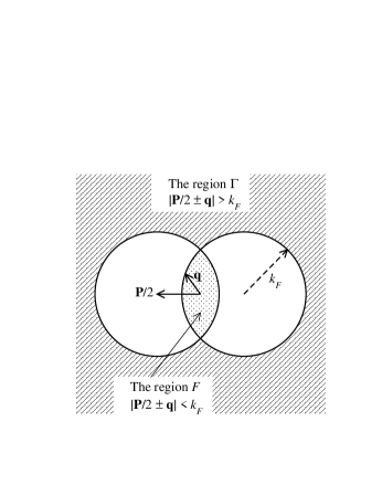
FIG. 3.: Integration regions $\Gamma$ and $F$.

The matrix elements of $\hat{\Gamma}_{\bf P}$ can be used to find the ground state energy per particle for a system of $A$ nucleons [30]:

$$\frac{E_{\rm g.s.}}{A}=\frac{3}{5}\,\frac{k_{F}^{2}}{2M}+\frac{E_{\rm int}}{A}\ ,$$ (43)

with

$$\frac{E_{\rm int}}{A}=\frac{g}{2\rho}\int_{F}\frac{d^{3}P\,d^{3}k}{(2\pi)^{6}}\left(g\langle{\bf k}|\hat{\Gamma}_{\bf P}|{\bf k}\rangle-\langle{\bf k}|\hat{\Gamma}_{\bf P}|{\bf-k}\rangle\right)\ .$$ (44)

Here $g=(2S+1)(2I+1)$ is the spin-isospin degeneracy factor, $\rho=gk_{F}^{3}/(6\pi^{2})$ is the density of nucleons, and the integration region $F$ is the intersection of the two Fermi spheres, as depicted in Fig. 3. We will use $E_{\rm g.s.}/A$ as our basic finite density observable.

We start with the DR/PDS effective field theory. Evaluating Eq. (44) to ${\cal O}(\alpha)$ is just the Hartree-Fock approximation; the relevant diagrams are shown in Fig. 4a. Both the EFT and true results can be analytically integrated and expanded (see Appendix C) to give (with $\xi\equiv k_{F}/m$)

$$\frac{E_{\rm int}^{(1)}}{A} = (g-1)\frac{\alpha m^{2}}{3\pi M}$$ (48)

$$\hbox{}\times\left\{\begin{array}[]{lc}\displaystyle\xi^{3}-\frac{3}{5}\xi^{5}+\frac{27}{70}\xi^{7}+{\cal O}(\xi^{9})\ ,&\quad\mbox{true}\\[8.0pt] \displaystyle\frac{Mm}{4\pi}\left[C_{0}^{(1)}\xi^{3}+\frac{3}{10}m^{2}C_{2}^{(1)}\xi^{5}+\frac{9}{70}m^{4}C_{4}^{(1)}\xi^{7}\right]+{\cal O}(\xi^{9})\ ,&\quad\mbox{EFT (DR/PDS)}\end{array}\right.$$

with terms only up to $C_{4}$ shown in the EFT calculation. As each new constant $C_{2n}$ is added to the effective potential and the values found in free space are used from Eqs. (19), (27), (29), and (30), the EFT result for $E_{\rm g.s.}/A$ coincides with the true result up to truncation errors of ${\cal O}(k_{F}^{2n+5})$ and ${\cal O}(\alpha^{2})$. There is no surprise here: The perturbative matching at finite density must work to this order since the EFT is merely parametrizing the Taylor expansion of $V_{\rm true}$ before the integration over the intersection of the Fermi spheres in Eq. (44).

FIG. 4.: Perturbative matching for the energy in nuclear matter at ${\cal O}(k_{F}^{5})$.

Taking the analysis to the next order in $\alpha$ requires an evaluation of the Pauli-blocked $\langle\hat{V}\hat{G}_{0}\hat{V}\rangle$ shown in Fig. 4b, and hence is a better test of how the EFT carries over to nuclear matter. The low-momentum part of the true and EFT integrals still agree up to ${\cal O}(k^{2n})$, since the non-Pauli-blocked part includes the same momentum states in each. If $k_{F}\ll m$, the Pauli blocking has no effect on the high-momentum parts of the integrals, which are therefore the same as in free-space. Thus the renormalization in free space of $C_{2n}^{(1)}$ by $C_{2n}^{(2)}$ carries over directly. Integrating over $F$ to find the energy leaves the same truncation error, ${\cal O}(k_{F}^{2n+5})$, as at order $\alpha$.

The steps involved in actually carrying out the integrations are outlined in Appendix C and the final expressions are given there. If we expand the energy per particle in powers of $\xi$, the true result is

$$\mbox{true:}\qquad\frac{E_{\rm int}^{(2)}}{A} = -(g-1)\frac{\alpha^{2}m^{2}}{6\pi M}$$ (51)

$$\hbox{}\times\biggl{[}\xi^{3}-\frac{12(11-2\ln 2)}{35\pi}\xi^{4}-\frac{3}{2}\xi^{5}+\frac{16(167/3-8\ln 2)}{105\pi}\xi^{6}$$

$$\quad\hbox{}+\frac{9}{5}\xi^{7}-\frac{4(26101/6-470\ln 2)}{1155\pi}\xi^{8}+{\cal O}(\xi^{9})\biggr{]}\ ,$$

and the EFT result using DR/PDS regularization is

$$\mbox{DR/PDS:}\;\;\frac{E_{\rm int}^{(2)}}{A} = -(g-1)\frac{\alpha^{2}m^{2}}{6\pi M}$$ (56)

$$\hbox{}\times\biggl{\{}\frac{Mm}{4\pi}\biggl{[}\left(-2C_{0}^{(2)}+\frac{M\mu}{2\pi}\left(C_{0}^{(1)}\right)^{2}\right)\xi^{3}-3Mm\left(C_{0}^{(1)}\right)^{2}\frac{(11-2\ln 2)}{35\pi^{2}}\xi^{4}$$

$$\quad\hbox{}-\frac{3}{5}\left(C_{2}^{(2)}-\frac{M\mu}{2\pi}\,C_{0}^{(1)}C_{2}^{(1)}\right)m^{2}\xi^{5}-Mm^{3}C_{0}^{(1)}C_{2}^{(1)}\frac{2(167/3-8\ln 2)}{105\pi^{2}}\xi^{6}$$

$$\quad\hbox{}-\frac{9}{35}\left(C_{4}^{(2)}-\frac{M\mu}{4\pi}\left(\left(C_{2}^{(1)}\right)^{2}+2C_{0}^{(1)}C_{4}^{(1)}\right)\right)m^{4}\xi^{7}-Mm^{5}C_{0}^{(1)}\widetilde{C}_{4}^{(1)}\frac{\xi^{8}}{5\pi^{2}}$$

$$\quad\hbox{}-Mm^{5}\left(2C_{0}^{(1)}C_{4}^{(1)}+\left(C_{2}^{(1)}\right)^{2}\right)\frac{(24715/6-470\ln 2)}{11550\pi^{2}}\xi^{8}\biggr{]}+{\cal O}(\xi^{9})\biggr{\}}\ .$$

Again, substitution of the expressions up to $C_{2n}$ from Eqs. (19), (27), and (29–31) removes the $\mu$ dependence and leads to agreement with the true result up to truncation errors of ${\cal O}(k_{F}^{2n+5})$. For a perturbative DR/PDS calculation with $k_{F}\ll m$, these errors are simply given by the first unmatched term in the expansion of the true result. For one constant the leading error is

$$\frac{\Delta E_{\rm int}}{A}=(g-1)\frac{m^{2}}{\pi M}\left(-\frac{1}{5}\alpha+\frac{1}{4}\alpha^{2}\right)\xi^{5}+{\cal O}(\xi^{6})\ ,$$ (57)

and for two constants it is

$$\frac{\Delta E_{\rm int}}{A}=(g-1)\frac{m^{2}}{\pi M}\frac{3}{10}\left(\frac{3}{7}\alpha-\alpha^{2}\right)\xi^{7}+{\cal O}(\xi^{8})\ .$$ (58)

The full error is depicted graphically in Fig. 5, which shows a similar breakdown scale to that in free space.

We emphasize that the contribution from the term in Eq. (56) proportional to $\widetilde{C}_{4}^{(1)}$ is needed to reproduce the $\xi^{8}$ term in Eq. (51). Since this coefficient does not contribute to on-shell two-body scattering, it might be interpreted as an “off-shell ambiguity.” However, as discussed above, it is determined by on-shell three-body scattering, so there is no need to consider off-shell effects in the two-body sector. At higher order in $\alpha$, we will need full three-body contact terms, matched in the three-body sector, to account for high-energy contributions [4].

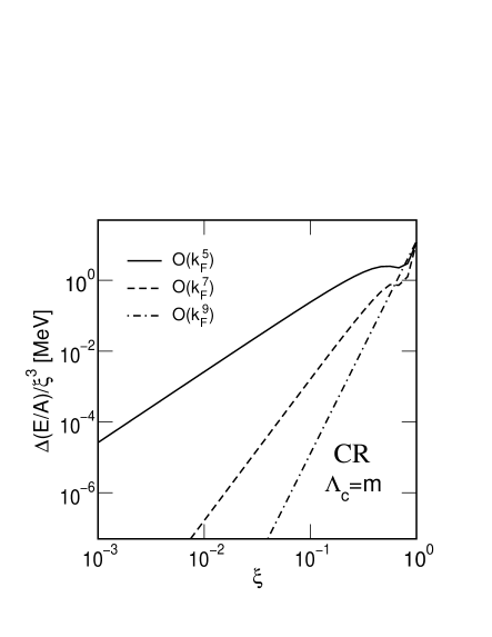
FIG. 5.: Error in the ground state energy per particle in nuclear matter to ${\cal O}(\alpha^{2})$ vs. $\xi\equiv k_{F}/m$ for $\alpha=-1/2$ with $M=940$ MeV and $m=600$ MeV. The error is divided by $\xi^{3}$ for clarity. Results for cutoff regularization (CR) with $\Lambda_{c}=m$ are shown on the left and for dimensional regularization (DR/PDS) on the right.

We find analogous results with cutoff regularization. The expanded ${\cal O}(\alpha)$ energy is (keeping terms to ${\cal O}(k^{2})$ in the effective potential):

$$\mbox{CR:}\quad\frac{E_{\rm int}^{(1)}}{A} = (g-1)\frac{\alpha m^{2}}{3\pi M}\left\{\frac{Mm}{4\pi}\left[C_{0}^{(1)}\xi^{3}+\frac{3}{10}m^{2}\left(C_{2}^{(1)}-\frac{1}{\Lambda_{c}^{2}}C_{0}^{(1)}\right)\xi^{5}\right]+{\cal O}(\xi^{7})\right\}$$ (59)

and using the explicit expression for $\delta C_{0}^{(2)}$ from Appendix B, the ${\cal O}(\alpha^{2})$ result is

$$\mbox{CR:}\;\;\frac{E_{\rm int}^{(2)}}{A} = -(g-1)\frac{\alpha^{2}m^{2}}{6\pi M}$$ (63)

$$\hbox{}\times\Biggl{\{}\frac{Mm}{4\pi}\Biggl{[}\left(-2C_{0}^{(2)}+\frac{M}{2\pi}\frac{\Lambda_{c}}{\sqrt{\pi}}\left(C_{0}^{(1)}\right)^{2}\right)\xi^{3}-3Mm\left(C_{0}^{(1)}\right)^{2}\frac{\left(11-2\ln 2\right)}{35\pi^{2}}\xi^{4}$$

$$\quad\hbox{}-\frac{3}{5}\Biggl{(}C_{2}^{(2)}-\frac{C_{0}^{(2)}}{\Lambda_{c}^{2}}-\frac{M}{2\pi}\frac{\Lambda_{c}}{\sqrt{\pi}}\left[-\frac{3}{2\Lambda_{c}^{2}}\left(C_{0}^{(1)}\right)^{2}+C_{0}^{(1)}C_{2}^{(1)}+\frac{3\Lambda_{c}^{2}}{16}\left(C_{2}^{(1)}\right)^{2}\right]\Biggr{)}m^{2}\xi^{5}$$

$$\quad\hbox{}-Mm^{3}\left(C_{0}^{(1)}C_{2}^{(1)}-\frac{1}{\Lambda_{c}^{2}}\left(C_{0}^{(1)}\right)^{2}\right)\frac{2(167/3-8\ln 2)}{105\pi^{2}}\xi^{6}\Biggr{]}+{\cal O}(\xi^{7})\Biggr{\}}\ .$$

These expressions parallel those found in the DR/PDS scheme in Eqs. (48) and (56). Taking the values for the constants found from matching in free-space (see Appendix B), and substituting them into Eqs. (59) and (63) produces $\Lambda_{c}$–independent results at each order in the momentum expansion (although the truncation error depends on $\Lambda_{c}$). The leading error for one constant is

$$\frac{\Delta E_{\rm int}}{A}=(g-1)\frac{m^{2}}{\pi M}\left(\left[-\frac{1}{5}+\frac{1}{10}\frac{m^{2}}{\Lambda_{c}^{2}}\right]\alpha+\left[\frac{1}{4}-\frac{1}{5}\left(\frac{m}{\sqrt{\pi}\Lambda_{c}}+\frac{1}{4}\frac{m^{2}}{\Lambda_{c}^{2}}\right)\right]\alpha^{2}\right)\xi^{5}+{\cal O}(\xi^{6})\ ,$$ (64)

and for two constants it is

$$\frac{\Delta E_{\rm int}}{A} = (g-1)\frac{m^{2}}{\pi M}\frac{3}{10}\Biggl{(}\left[\frac{3}{7}-\frac{2}{7}\frac{m^{2}}{\Lambda_{c}^{2}}+\frac{1}{14}\frac{m^{4}}{\Lambda_{c}^{4}}\right]\alpha$$ (67)

$$\hbox{}+\left[-1+\frac{4}{7\sqrt{\pi}}\frac{m}{\Lambda_{c}}+\frac{5}{14}\frac{m^{2}}{\Lambda_{c}^{2}}-\frac{5}{21\sqrt{\pi}}\frac{m^{3}}{\Lambda_{c}^{3}}-\frac{1}{28}\frac{m^{4}}{\Lambda_{c}^{4}}+\frac{4}{7\sqrt{\pi}}\frac{\Lambda_{c}}{m}\right]\alpha^{2}\Biggr{)}\xi^{7}$$

$$\hbox{}+{\cal O}(\xi^{8})\ .$$

Just as in the DR/PDS case, the error decreases by a power of $\xi^{2}$ for each additional order, as shown in Fig. 5. This again shows the breakdown scale at finite density is similar to the breakdown scale in free space.

In summary, at finite density the energy per particle has similar error plots to those in free-space when $\Delta E_{\rm g.s.}/A$ is plotted against the Fermi momentum $k_{F}$. The improvement is by two powers of $k_{F}$ with each additional order (although both even and odd powers of $k_{F}$ are present in the energy per particle). The apparent breakdown scale is still $\Lambda\approx m$, without any numerical factors significantly different from unity. The important observation is not the precise breakdown scale, which depends on the details of the underlying interaction, but that the breakdown in free space and in the medium are closely related. The analysis is easily extended to higher partial waves for both regularization schemes, which verifies the matching and the conclusions about the breakdown scale.

IV Discussion

The model we have studied shows that an EFT expansion for NN scattering leads to a low-density expansion of the energy per nucleon in nuclear matter. In particular, in the former one finds scattering observables order-by-order in the nucleon relative momentum over a breakdown scale [2]. In the latter, one finds the energy per particle order-by-order in the Fermi momentum $k_{F}$ over essentially the same scale. We have checked that this basic conclusion is independent of the details of the model potential. We expect that this type of expansion will also result when long-distance pion physics is explicitly included, in analogy to the modified effective range expansion in free space [20].

Of course, since this is a perturbative calculation it can only be suggestive. We will need to clarify a variety of interrelated issues: nonperturbative power counting in the medium, the impact of pions, the elimination of off-shell ambiguities, the role of three-nucleon interactions. However, if we assume the basic results here carry over to a full nonperturbative treatment, we can speculate on how well a leading order (LO) and next-to-leading order (NLO) EFT calculation will do in reproducing nuclear matter saturation.

In particular, we can use phenomenological energy functionals of nuclear matter (that is, the energy expressed as a function of the density) to anticipate what a full EFT calculation might achieve. Nonrelativistic and relativistic mean-field functionals provide parameterizations of the energy per particle near the equilibrium density, with individual contributions characterized by a density expansion parameter of about 1/5 [32]. These functionals are fit directly to finite density data. As such, they include (approximately) the effects of three-body forces and short-range correlations, even though the formalism is that of Hartree or Hartree-Fock [32]. (There are certainly important limitations in the descriptions; for example, there is no $k_{F}^{4}$ term in nonrelativistic mean-field energy functionals.)

If we assume that the expansions about $k_{F}=0$ are reasonably determined by fits near $(k_{F})_{\rm equilibrium}<\Lambda$, then we can use them to predict how far in a truncated $k_{F}$ expansion we need to go to see saturation. Ordinary Skyrme Hartree-Fock functionals are truncated at $\rho^{3}$, which is $\rho^{2}\propto k_{F}^{6}$ in the energy per particle. As more terms are added to the functional, it should become a more reliable “extrapolation” of an expansion about $k_{F}=0$. So we can look at a generalized Skyrme model, fit out to $k_{F}^{9}$ but then truncated at $k_{F}^{6}$, to see how saturation changes. In this case, the equilibrium density decreases by about 20% while the binding energy decreases by roughly 5 MeV [33]. There is an energy minimum when only terms up through $k_{F}^{5}$ is kept, but it is far removed from the empirical point. Thus we expect a qualitative reproduction of saturation if we keep terms up through $k_{F}^{6}$, as long as the effective $\Lambda$ is sufficiently high.

A similar conclusion is reached by examining relativistic mean-field point-coupling models. These models contain contributions to all orders in the $k_{F}$ expansion. One finds that a saturation minimum is first achieved with an expansion truncated at $k_{F}^{5}$ but that the $k_{F}^{6}$ term is needed to get reasonably close. The quantitative results again suggest that an EFT calculation up to $k_{F}^{6}$ might reproduce nuclear saturation with the equilibrium binding energy given to within about 5 MeV and the density to within about 20%.

The mass scale that sets the convergence of contributions to mean-field energy functionals is of order 600 MeV [32]. However, this is not necessarily the same as the breakdown scale. If one constructs error plots for relativistic mean-field functionals by comparing the full energy as a function of $k_{F}$ to the same functional truncated at $k_{F}^{5}$, at $k_{F}^{6}$, and so on, a breakdown scale for the expansion about $k_{F}=0$ is identified. For point-coupling models, this breakdown scale is close to 400 MeV but for models with meson fields it is actually below the equilibrium $k_{F}$ [34]. This discrepancy is not yet understood.

One might ask how saturation is realized in such a density expansion. The existence of a minimum in the energy per particle suggests that different orders in the expansion must be playing off each other; a natural conclusion is that this should only occur near the breakdown scale (where all terms contribute equally) and not at $k_{F}\ll\Lambda$. The mean-field phenomenology suggests a resolution: there is an interplay of different orders but it is highly restricted. In particular, repulsion from the $k_{F}^{5}$ and $k_{F}^{6}$ terms becomes important compared to the attraction from the $k_{F}^{3}$ piece well below the breakdown scale $\Lambda$. Furthermore, this happens because the coefficient of the $k_{F}^{3}$ term is unnaturally small; in relativistic models this is a direct result of cancellations between Lorentz scalar and vector contributions that are each of natural size. The cancellations leading to a small $k_{F}^{3}$ term do not recur in higher orders, so further contributions just correct the equilibrium properties and do not change the qualitative behavior.

The convergence of the density expansion is also consistent with the convergence of a conventional expansion of the Galitskii equation in powers of $k_{F}$ times the radius of a strong, short-range (hard-core) potential[30], which we can associate with $1/\Lambda$. In the effective field theory treatment, this short-distance expansion parameter arises naturally when long-distance pion physics is treated explicitly. In free space, consistently including the pion takes us from an effective range expansion with a breakdown scale of order the pion mass to a modified effective range expansion with a breakdown scale set by the next important mass scale. We expect an analogous situation at finite density.

So what are the ingredients of a minimal EFT calculation of nuclear matter saturation? First, we need the breakdown scale for NN scattering in free space to be as large as possible. There are indications that a complete NLO calculation using cutoff regularization and including two-pion irreducible contributions (and possibly the NNLO two-pion pieces) may achieve $\Lambda\approx 600\,\mbox{MeV}$ [23]. Then we must include all contributions that will generate terms in the energy per particle up to $k_{F}^{6}$. This implies including two constants in each S-wave, one in each P-wave, and an S–D mixing term. One- and two-pion exchange should be included in all waves. Finally, a three-body contact term will be needed [4]. Note that this recipe includes the standard ingredients of nuclear matter phenomenology: the pion tensor force, velocity dependence of the interaction, mid-range attraction from two-pion exchange, and three-body forces. While much remains to be done before a consistent nonperturbative calculation is available, we are optimistic that our speculations will be tested in the near future.

A Nonperturbative Free-Space Solutions

Scattering from the $S$–wave separable potential

$$\langle{\bf k^{\prime}}|\hat{V}_{\rm true}|{\bf k}\rangle=\frac{4\pi m}{M}\frac{\alpha m^{2}}{(k^{2}+m^{2})(k^{\prime}{}^{2}+m^{2})}\equiv V_{0}(k,k^{\prime})\ ,$$ (A1)

can be solved analytically to give

$$T_{0}^{-1}(k,k)=V_{0}^{-1}(k,k)+\frac{M}{4\pi}\left(ik-\frac{k^{2}-m^{2}}{2m}\right)$$ (A2)

or

$$k\cot\delta_{0}=-\frac{4\pi}{MV_{0}(k,k)}+\frac{k^{2}-m^{2}}{2m}\ .$$ (A3)

Expanding $k\cot\delta_{0}$ in powers of $k^{2}$ gives the effective range expansion for this potential:

$$k\cot\delta_{0}=-m\left(\frac{1}{2}+\frac{1}{\alpha}\right)+\frac{1}{m}\left(\frac{1}{2}-\frac{2}{\alpha}\right)k^{2}-\frac{1}{\alpha m^{3}}k^{4}\ .$$ (A4)

The effective-range parameters are natural (i.e., characterized by the underlying mass scale) for $\alpha={\cal O}(1)$.

Regularizing the EFT with DR/PDS gives

$$k\cot\delta_{0}^{\rm PDS}=-\frac{4\pi}{MV_{0}^{\rm PDS}(k,k)}-\mu\ ,$$ (A5)

which can readily be expanded in momentum and solved for the $S$–wave low-energy constants $C_{2n}$:

$$C_{0}=\frac{4\pi\alpha}{Mm}\left[1+\alpha\left(\frac{1}{2}-\frac{\mu}{m}\right)\right]^{-1}\!\!\!\!\!\!\ ,\;\;\;C_{2}=-\frac{C_{0}^{\;2}}{\alpha}\frac{M}{2\pi m}\left(1-\frac{\alpha}{4}\right)\ ,\;\;\;C_{4}=\frac{C_{2}^{\;2}}{C_{0}}-\frac{C_{0}^{\;2}}{\alpha}\frac{M}{4\pi m^{3}}\ .$$ (A6)

Expanding these results in powers of $\alpha$ gives the results in Eqs. (19), (27), and (29–30). Matching the tree-level on-shell three-body scattering amplitude [4] to leading order in $\alpha$ gives $\widetilde{C}_{4}=C_{0}/m^{4}$.

B Two Constants with Cutoff Regularization

For two terms in the effective potential, the expression for $C_{0}^{(2)}$ [Eq. (14)] gets an extra piece:

$$\delta C_{0}^{(2)}=\frac{M}{4\pi}\frac{\Lambda_{c}^{3}}{2\sqrt{\pi}}\left(C_{0}^{(1)}C_{2}^{(1)}+{3\over 8}\bigl{(}C_{2}^{(1)}\bigr{)}^{2}\Lambda_{c}^{2}\right)\ ,$$ (B1)

with

$$C_{2}^{(1)}=-\left(\frac{4\pi}{Mm}\right)\frac{2}{m^{2}}+\frac{C_{0}^{(1)}}{\Lambda_{c}^{2}}\ .$$ (B2)

The ${\cal O}(\alpha^{2})$ piece of $C_{2}$ has more terms compared to the DR/PDS result Eq. (29):

$$C_{2}^{(2)} = \left(\frac{4\pi}{Mm}\right)\frac{5}{2m^{2}}-\frac{M}{4\pi}\frac{\Lambda_{c}}{\sqrt{\pi}}\left(\frac{3}{\Lambda_{c}^{2}}\left(C_{0}^{(1)}\right)^{2}-2C_{0}^{(1)}C_{2}^{(1)}-\frac{3}{8}\left(C_{2}^{(1)}\right)^{2}\Lambda_{c}^{2}\right)+\frac{C_{0}^{(2)}}{\Lambda_{c}^{2}}\ .$$ (B3)

C Nuclear Matter Integrals

For an even-parity potential, Eqs. (41) and (44) give the first-order contribution to the energy per particle as

$$\frac{E_{\rm int}^{(1)}}{A}=\frac{g\,(g-1)}{2\rho}\int_{F}\frac{d^{3}P\,d^{3}k}{(2\pi)^{6}}\,\langle{\bf k}|\hat{V}|{\bf k}\rangle\equiv\frac{g\,(g-1)}{\pi^{4}\rho}\,m^{4}{\cal I}\ .$$ (C1)

For an odd-parity potential, the degeneracy pre-factor becomes $g(g+1)$. Introducing scaled momenta ${\bf s}\equiv\frac{1}{2}{\bf P}/k_{F}$ and ${\bf t}={\bf k}/k_{F}$, then

$${\cal I}=\xi^{4}\int_{0}^{1}ds\,s^{2}\int_{0}^{1}dx\int_{0}^{z_{-}(x)}dt\,t^{2}\,{\cal F}(t)\ ,$$ (C2)

with

$$z_{\pm}(x)\equiv\pm sx+\sqrt{1-s^{2}(1-x^{2})}\ ,\qquad\qquad{\cal F}(t)\equiv k_{F}^{2}\,\langle k_{F}{\bf t}|\hat{V}|k_{F}{\bf t}\rangle\ .$$ (C3)

Integrating by parts with respect to $x$ and then $s$, and changing variables simplifies the integral to

$${\cal I}=\frac{\xi^{4}}{6}\int_{0}^{1}\!\!ds\,s^{2}\left[2-3s+s^{3}\right]{\cal F}(s)\ ,$$ (C4)

which for the potential in Eq. (1) gives

$${\cal I}=\alpha\frac{2\pi m}{3M}\left[\xi^{2}+\xi^{3}\arctan\xi-\left(1+\frac{3}{2}\xi^{2}\right)\ln\left(1+\xi^{2}\right)\right]\ .$$ (C5)

The integral can also be directly evaluated for the DR/PDS and CR effective potentials.

The second-order contribution $E_{\rm int}^{(2)}/A$ follows from the same analysis as above, but with

$${\cal F}(t)=k_{F}^{3}\;{\cal P}\,\int_{\Gamma}\!\frac{d^{3}u}{(2\pi)^{3}}\langle k_{F}{\bf t}|\hat{V}|k_{F}{\bf u}\rangle\frac{M}{t^{2}-u^{2}}\langle{k_{F}\bf u}|\hat{V}|k_{F}{\bf t}\rangle\equiv\int_{0}^{1}dy\int_{z_{+}(y)}^{\infty}\!du\,u^{2}{\cal H}(t,u)\ ,$$ (C6)

where

$${\cal H}(t,u)=\frac{Mk_{F}^{3}}{2\pi^{2}}\langle k_{F}{\bf t}|\hat{V}|k_{F}{\bf u}\rangle\frac{1}{t^{2}-u^{2}}\langle{k_{F}\bf u}|\hat{V}|k_{F}{\bf t}\rangle\ .$$ (C7)

We divide the integrals into two parts:

$${\cal I}={\cal I}_{1}-{\cal I}_{2}\ ,$$ (C8)

with

$${\cal I}_{1} = \int_{0}^{1}ds\,s^{2}\int_{0}^{1}dx\int_{0}^{z_{-}(x)}dt\,t^{2}\int_{0}^{\infty}du\,u^{2}{\cal H}(t,u)\ ,$$ (C9)

$${\cal I}_{2} = \int_{0}^{1}ds\,s^{2}\int_{0}^{1}dx\int_{0}^{z_{-}(x)}dt\,t^{2}\int_{0}^{1}dy\int_{0}^{z_{+}(y)}du\,u^{2}{\cal H}(t,u)\ .$$ (C10)

The first integral ${\cal I}_{1}$ can be evaluated as in Eq. (C4). For the potential Eq. (1), this leads to

$${\cal I}_{1} = \alpha^{2}\left(\frac{\pi m}{6M}\right)\left[\ln\left(1+\xi^{2}\right)-\frac{\xi^{2}\left(2+\xi^{2}\right)}{2\left(1+\xi^{2}\right)}\right]$$ (C11)

$$= \alpha^{2}\left(\frac{\pi m}{6M}\right)\left[-\frac{\xi^{6}}{6}+\frac{\xi^{8}}{4}-\frac{3\xi^{10}}{10}+{\cal O}(\xi^{12})\right]\ .$$ (C12)

The second integral ${\cal I}_{2}$ is not conveniently expressed in closed form. For the potential Eq. (1), it can be expanded in $\xi$ to give

$${\cal I}_{2} = \alpha^{2}\left(\frac{m}{105M}\right)\biggl{[}-\xi^{7}(11-2\ln 2)+\frac{4\xi^{9}}{9}\left(\frac{167}{3}-8\ln 2\right)$$ (C14)

$$\qquad\hbox{}-\frac{\xi^{11}}{99}\left(\frac{26101}{6}-470\ln 2\right)+{\cal O}(\xi^{13})\biggr{]}\ .$$

Results for the EFT are found similarly.

REFERENCES

- [1] R. Machleidt, Adv. Nucl. Phys. 19 (1989) 189, and references therein.
- [2] Proceedings of the Joint Caltech/INT Workshop: Nuclear Physics with Effective Field Theory, ed. R. Seki, U. van Kolck, and M.J. Savage (World Scientific, 1998).
- [3] D.B. Kaplan, M.J. Savage, M.B. Wise Phys. Rev. C59 (1999) 617.
- [4] P.F. Bedaque, H.–W. Hammer, and U. van Kolck, Phys. Rev. C 58 (1998) R641; Nucl. Phys. A646 (1999) 444.
- [5] J.V. Steele and R.J. Furnstahl, “Describing nuclear matter with effective field theory,” e-print nucl-th/9908005.
- [6] W. Lin and B.D. Serot, Nucl. Phys. A512 (1990) 637.
-
[7]
U. van Kolck, Ph.D. thesis, U. Texas, Aug. 1993;
C. Ordonez, L. Ray, and U. van Kolck, Phys. Rev. Lett. 72 (1994) 1982; Phys. Rev. C53 (1996) 2086. - [8] W.E. Caswell and G.P. Lepage, Phys. Lett. 167B, 437 (1986).
- [9] T.H.R. Skyrme, Phil. Mag. 1 (1956) 1043; Nucl. Phys. 9 (1959) 615.
-
[10]
J.W. Negele, Phys. Rev. C1 (1970) 1260;
J.W. Negele and D. Vautherin, Phys. Rev. C5 (1972) 1472;
J.W. Negele, Rev. Mod. Phys. 54 (1982) 913. - [11] M.I. Haftel and F. Tabakin, Nucl. Phys. A158 (1970) 1.
- [12] R. Shankar, Rev. Mod. Phys. 66 (1994) 129; “Effective field theory in condensed matter physics,” e-print cond-mat/9703210.
- [13] J. Hormuzdiar and S.D.H. Hsu, “Effective field theory of neutron star superfluidity,” e-print nucl-th/9811017.
-
[14]
M. Lutz, Nucl. Phys. A642 (1998) 171c;