Shell Corrections of Superheavy Nuclei in Self-Consistent Calculations

Abstract

Shell corrections to the nuclear binding energy as a measure of shell effects in superheavy nuclei are studied within the self-consistent Skyrme-Hartree-Fock and Relativistic Mean-Field theories. Due to the presence of low-lying proton continuum resulting in a free particle gas, special attention is paid to the treatment of single-particle level density. To cure the pathological behavior of shell correction around the particle threshold, the method based on the Green’s function approach has been adopted. It is demonstrated that for the vast majority of Skyrme interactions commonly employed in nuclear structure calculations, the strongest shell stabilization appears for $Z$=124, and 126, and for $N$=184. On the other hand, in the relativistic approaches the strongest spherical shell effect appears systematically for $Z$=120 and $N$=172. This difference has probably its roots in the spin-orbit potential. We have also shown that, in contrast to shell corrections which are fairly independent on the force, macroscopic energies extracted from self-consistent calculations strongly depend on the actual force parametrisation used. That is, the $A$ and $Z$ dependence of mass surface when extrapolating to unknown superheavy nuclei is prone to significant theoretical uncertainties.

]

I Introduction

The stability of the heaviest and superheavy elements has been a long-standing fundamental question in nuclear science. Theoretically, the mere existence of the heaviest elements with $Z$$>$104 is entirely due to quantal shell effects. Indeed, for these nuclei the shape of the classical nuclear droplet, governed by surface tension and Coulomb repulsion, is unstable to surface distortions driving these nuclei to spontaneous fission. That is, if the heaviest nuclei were governed by the classical liquid drop model, they would fission immediately from their ground states due to the large electric charge. However, in the mid-sixties, with the invention of the shell-correction method, it was realized that long-lived superheavy elements (SHE) with very large atomic numbers could exist due to the strong shell stabilization [1, 2, 3, 4].

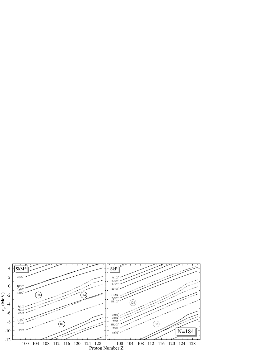
FIG. 1.: Single-proton levels for $N$=184 isotones with 110$\leq$$Z$$\leq$130 calculated in the Skyrme-Hartree-Fock model with SkM^∗ (left) and SkP effective interactions. Positive (negative) parity levels are indicated by solid (dashed) lines and by their spherical labels ($nlj$). Note that in both cases the nucleus $Z$=126 is proton-unbound, i.e., the $p_{1/2}$ shell has positive energy.

In spite of tremendous experimental effort, after about thirty years of the quest for superheavy elements, the borders of the upper-right end of the nuclear chart are still unknown [5]. However, it has to be emphasized that the recent years also brought significant progress in the production of the heaviest nuclei [5, 6]. During 1995-96, three new elements, $Z$=110, 111, and 112, were synthesized by means of both cold and hot fusion reactions [7, 8, 9, 10]. These heaviest isotopes decay predominantly by groups of $\alpha$ particles ($\alpha$ chains) as expected theoretically [11, 12, 13]. Recently, two stunning discoveries have been made. Firstly, hot fusion experiments performed in Dubna employing ⁴⁸Ca+²⁴⁴Pu and ⁴⁸Ca+²⁴²Pu “hot fusion” reactions [14] gave evidence for the synthesis of two isotopes ($A$=287 and 289) of the element $Z$=114. Secondly, the Berkeley-Oregon team, utilizing the “cold fusion” reaction ⁸⁶Kr+²⁰⁸Pb [15], observed three $\alpha$-decay chains attributed to the decay of the new element $Z$=118, $A$=293. The measured $\alpha$-decay chains ²⁸⁹114 and ²⁹³118 turned out to be consistent with predictions of the Skyrme-Hartree-Fock (SHF) theory [16] and the Relativistic Mean-Field (RMF) theory [17].

The goal of the present work is to study shell closures in SHE. To that end we use as a tool microscopic shell corrections extracted from self-consistent calculations. For medium-mass and heavy nuclei, self-consistent mean-field theory is a very useful starting point [18]. Nowadays, SHF and RMF calculations with realistic effective forces are able to describe global nuclear properties with an accuracy which is comparable to that obtained in more phenomenological macroscopic-microscopic models based on the shell-correction method.

In previous work [19], shell energies for SHE elements were extracted by subtracting from calculated HF binding energies the macroscopic Yukawa-plus-exponential mass formula [20] with parameters of Ref. [21]. In another work, based on the RMF theory [22], shell corrections were extracted for the heaviest deformed nuclei using the standard Strutinsky method in which the positive-energy spectrum was approximated by quasi-bound states. Neither procedure can be considered as satisfactory. A proper treatment of continuum states is achieved with a Green’s function method [23]. We employ this method for the present study of shell corrections of SHE.

The material contained in this study is organized as follows. The motivation of this work is outlined in Sect. II, Section III contains a brief discussion of the Strutinsky energy theorem on which the concept of shell correction is based. The Green’s Function HF method used to extract the single-particle level density is presented in Sect. IV. Section V discusses the details of our HF and RMF models and describes the Strutinsky procedure employed. The results of calculations for shell corrections in spherical SHE and for macroscopic energies extracted from self-consistent binding energies are discussed in Sec. VI. Finally, Sec. VII contains the main conclusions of this work.

II Motivation

All the heaviest elements found recently are believed to be well deformed. Indeed, the measured $\alpha$-decay energies, along with complementary syntheses of new neutron-rich isotopes of elements $Z$=106 and $Z$=108, have furnished confirmation of the special stability of the deformed shell at $N$=162 predicted by theory [24, 25]. Beautiful experimental confirmation of large quadrupole deformations in this mass region comes from gamma-ray spectroscopy. Recent experimental works [26, 27] succeeded in identifying the ground-state band of ²⁵⁴No (the heaviest nucleus studied in gamma-ray spectroscopy so far). The quadrupole deformation of ²⁵⁴No, inferred from the energy of the deduced $2^{+}$ state, is in nice agreement with theoretical predictions [19, 21, 28, 29]. Still heavier and more neutron-rich elements are expected to be spherical due to the proximity of the neutron shell at $N$=184. This is the region of SHE which we will investigate here.

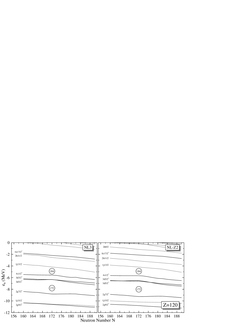
FIG. 2.: Single-neutron levels for $Z$=120 isotopes with 160$\leq$$N$$\leq$190 calculated in the RMF approach with NL3 (left) and NL-Z2 non-linear parametrizations. The line convention is the same as in Fig. 1. Note large neutron gaps at $N$=172 and 184.

In spite of an impressive agreement with available experimental data for the heaviest elements, theoretical uncertainties are large when extrapolating to unknown nuclei with greater atomic numbers. As discussed in Refs.  [19, 30], the main factors that influence the single-proton shell structure of SHE are (i) the Coulomb potential and (ii) the spin-orbit splitting. As far as the protons are concerned, the important spherical shells are the closely spaced $1i_{13/2}$ and $2f_{7/2}$ levels which appear just below the $Z$=114 gap, the $2f_{5/2}$ shell which becomes occupied at $Z$=120, the $3p_{3/2}$ shell which becomes occupied at $Z$=124, and the $3p_{1/2}$ and $1i_{11/2}$ orbitals whose splitting determines the size of the $Z$=126 magic gap. Interestingly, while the ordering of single-proton states is practically the same for all the self-consistent approaches with realistic effective interactions (see Fig. 1 and single-particle diagrams in Refs. [19, 30]), their relative positions vary depending on the choice of force parameters. Since in the region of SHE the single-particle level density is relatively large, small shifts in positions of single-particle levels can influence the strength of single-particle gaps and be crucial for determining the shell stability of a nucleus. As a result, there is no consensus between theorists concerning the next proton magic gap beyond $Z$=82. While most macroscopic-microscopic (non-self-consistent) approaches predict $Z$=114 to be magic, self-consistent calculations suggest that the center of the proton shell stability should be moved up to higher proton numbers, $Z$=120, 124 or 126 [19, 29, 30, 31]. It is to be noted that the Coulomb potential mainly influences the magnitude of the $Z$=114 gap. (Here, the self-consistent treatment of Coulomb energy is a key factor.) On the other hand, the spin-orbit interaction determines the position of the $2f$ and $3p$ shells which define the proton shell structure above $Z$$>$114.

The spherical neutron shell structure is governed by the following orbitals: $1j_{15/2}$ (below the $N$=164 gap), $2g_{7/2}$, $3d_{5/2}$, $3d_{3/2}$, and $4s_{1/2}$ and $1j_{13/2}$ whose splitting determines the size of the $N$=184 spherical gap (see Fig. 2 and Refs. [19, 30]). Again, similar to the proton case, the order of the single-neutron orbitals between $N$=164 and 184 is rather robust, while sizes of single-particle gaps vary. For instance, the $N$=172 gap, predicted by the RMF calculations shown in Fig. 2, results from the large energy splitting between the $2g_{7/2}$ and $3d_{5/2}$ shells. In non-relativistic models, these two orbitals are very close in energy, and this degeneracy is related to the pseudo-spin symmetry [32, 33]. Interestingly, in the SHF calculations, the pseudo-spin degeneracy holds in most cases. Namely, certain neutron orbitals group in pairs (pseudo-spin doublets): ($2g_{7/2}$, $3d_{5/2}$), ($3d_{3/2}$, $4s_{1/2}$), and the same holds for proton orbitals, e.g., ($2f_{5/2}$, $3p_{3/2}$). Considering the fact that the idea of pseudo-spin has relativistic roots [34, 35], it is surprising to see that this symmetry is so dramatically violated in the RMF theory. As a matter of fact, the presence of pronounced magic gaps at $Z$=120 and $N$=172 in RMF models (see below) is a direct manifestation of the pseudo-spin symmetry breaking.

As discussed in Ref. [19], neutron-deficient superheavy nuclei are expected to be unstable to proton emission. Indeed, as seen in Fig. 1, the proton $3p_{1/2}$ shell has positive energy for $Z$$\geq$126, i.e., in these nuclei the $3p_{1/2}$ level is a narrow resonance. Due to huge Coulomb barriers, superheavy nuclei with $Q_{p}$$<$1.5 MeV are practically proton-stable [19]. However, the higher-lying single-proton orbitals are expected to have sizable proton widths.

In order to assess the magnitude of shell effects determined by the bunchiness of single-particle levels, it is useful to apply the Strutinsky renormalization procedure [36, 37, 38] which makes it possible to calculate the shell correction energy. Unfortunately, the standard way of extracting shell correction breaks down for weakly bound nuclei where the contribution from the particle continuum becomes important [39]. Recently, a new method of calculating shell correction, based on the correct treatment of resonances, has been developed [40, 41]. The improved method is based on the theory of Gamow states (eigenstates of one-body Hamiltonian with purely outgoing boundary conditions) which can be calculated numerically for commonly used optical-model potentials [42]. While this “exact” procedure cannot be easily adopted to the case of microscopic self-consistent potentials, its simplified version applying the Green’s-function method can [23].

III Shell Correction and the Energy Theorem

The main assumption of the shell-correction (macroscopic-microscopic) method [36, 37, 38, 43] is that the total energy of a nucleus can be decomposed into two parts:

$$E=\tilde{E}+E_{\rm shell},$$ (1)

where $\tilde{E}$ is the macroscopic energy (smoothly depending on the number of nucleons and thus associated with the “uniform” distribution of single-particle orbitals) and $E_{\rm shell}$ is the shell-correction term that fluctuates with particle number reflecting the non-uniformities (bunchiness) of the single-particle level distribution. In order to make a separation (1), one starts from the one-body HF density matrix $\rho$

$${\rho}(\mathchoice{{\hbox{\boldmath$\displaystyle r$}}}{{\hbox{\boldmath$\textstyle r$}}}{{\hbox{\boldmath$\scriptstyle r$}}}{{\hbox{\boldmath$\scriptscriptstyle r$}}}^{\prime},\mathchoice{{\hbox{\boldmath$\displaystyle r$}}}{{\hbox{\boldmath$\textstyle r$}}}{{\hbox{\boldmath$\scriptstyle r$}}}{{\hbox{\boldmath$\scriptscriptstyle r$}}})=\sum_{i}n_{i}\phi_{i}(\mathchoice{{\hbox{\boldmath$\displaystyle r$}}}{{\hbox{\boldmath$\textstyle r$}}}{{\hbox{\boldmath$\scriptstyle r$}}}{{\hbox{\boldmath$\scriptscriptstyle r$}}}^{\prime})\phi^{*}_{i}(\mathchoice{{\hbox{\boldmath$\displaystyle r$}}}{{\hbox{\boldmath$\textstyle r$}}}{{\hbox{\boldmath$\scriptstyle r$}}}{{\hbox{\boldmath$\scriptscriptstyle r$}}}),$$ (2)

which can be decomposed into a “smoothed” density $\tilde{\rho}$ and a correction $\delta\rho$, which fluctuates with the shell filling

$$\rho=\tilde{\rho}+\delta\rho.$$ (3)

In Eq. (2), $n_{i}$ is the single-particle occupation coefficient which is equal to 1(0) if the level $e_{i}$ is occupied (empty). The smoothed single-particle density $\tilde{\rho}$ can be expressed by means of the smoothed distribution numbers $\tilde{n}_{i}$ [44]:

$${\tilde{\rho}}(\mathchoice{{\hbox{\boldmath$\displaystyle r$}}}{{\hbox{\boldmath$\textstyle r$}}}{{\hbox{\boldmath$\scriptstyle r$}}}{{\hbox{\boldmath$\scriptscriptstyle r$}}}^{\prime},\mathchoice{{\hbox{\boldmath$\displaystyle r$}}}{{\hbox{\boldmath$\textstyle r$}}}{{\hbox{\boldmath$\scriptstyle r$}}}{{\hbox{\boldmath$\scriptscriptstyle r$}}})=\sum_{i}\tilde{n}_{i}\phi_{i}(\mathchoice{{\hbox{\boldmath$\displaystyle r$}}}{{\hbox{\boldmath$\textstyle r$}}}{{\hbox{\boldmath$\scriptstyle r$}}}{{\hbox{\boldmath$\scriptscriptstyle r$}}}^{\prime})\phi^{*}_{i}(\mathchoice{{\hbox{\boldmath$\displaystyle r$}}}{{\hbox{\boldmath$\textstyle r$}}}{{\hbox{\boldmath$\scriptstyle r$}}}{{\hbox{\boldmath$\scriptscriptstyle r$}}}).$$ (4)

When considered as a function of the single-particle energies $e_{i}$, the numbers $\tilde{n}_{i}$ vary smoothly in an energy interval of the order of the energy difference between major shells. The averaged HF Hamiltonian $\tilde{h}_{\rm HF}$ can be directly obtained from $\tilde{\rho}$. The expectation value of a HF Hamiltonian (containing the kinetic energy, $t$ and the two-body interaction, $\bar{v}$) can then be written in terms of $\tilde{\rho}$ and $\delta\rho$ [43, 45]:

$$E_{\rm HF}={\rm Tr}(t\rho)+{1\over 2}{\rm Tr\,Tr}(\rho\bar{v}\rho)=\tilde{E}+E_{\rm osc}+O(\delta\rho^{2}),$$ (5)

where

$$\tilde{E}={\rm Tr}(t\tilde{\rho})+{1\over 2}{\rm Tr\,Tr}(\tilde{\rho}\bar{v}\tilde{\rho})$$ (6)

is the average part of $E_{\rm HF}$ and

$$E_{\rm osc}={\rm Tr}(\tilde{h}_{\rm HF}\delta\rho)\quad\mbox{with}\quad\tilde{h}_{\rm HF}=t+{\rm Tr}(\bar{v}\tilde{\rho})$$ (7)

is the first-order term in $\delta\rho$ representing the shell-correction contribution to $E_{\rm HF}$. If a deformed phenomenological potential gives a similar spectrum to the averaged HF potential $\tilde{h}_{\rm HF}$, then the oscillatory part of $E_{\rm HF}$, given by Eq. (7), is very close to that of the deformed shell model, $E_{\rm shell}$=$E_{\rm osc}+O(\delta\rho^{2})$. The second-order term in Eq. (5) is usually very small and can be neglected [46]. The above relation, known as the Strutinsky Energy Theorem, makes it possible to calculate the total energy using the non-self-consistent, deformed independent-particle model; the average part $\tilde{E}$ is usually replaced by the corresponding phenomenological liquid-drop (or droplet) model value, $E_{\rm macro}$. It is important that $E_{\rm shell}$ must not contain any regular (smooth) terms analogous to those already included in the phenomenological macroscopic part. The numerical proof of the Energy Theorem was carried out by Brack and Quentin [47] who demonstrated that Eq. (1) holds for $E_{\rm shell}$ defined by means of the smoothed single-particle energies (eigenvalues of $\tilde{h}_{\rm HF}$).

In this work, we use a simpler expression to extract the shell correction from the HF binding energy, which should also be accurate up to $O(\delta\rho^{2})$. Namely, as an input to the Strutinsky procedure we take the self-consistent single-particle HF energies, $e^{\rm HF}_{i}$. In this case, the shell correction is given by

$${E}_{\rm shell}(\rho)=\sum_{i}(n_{i}-\tilde{n}_{i})e_{i}+O(\delta\rho^{2}).$$ (8)

The equivalent macroscopic energy can easily be computed by taking the difference

$$E_{\rm macro}\approx\tilde{E}^{\rm HF}=E(\rho)-{E}_{\rm shell}(\rho).$$ (9)

IV Green’s Function Hartree-Fock Approach to Shell Correction

The HF equation is generally solved using a harmonic oscillator expansion method or by means of a discretization in a three-dimensional box. In both cases, a great number of unphysical states with positive energy appear. The effect of these quasi-bound states is disastrous for the Strutinsky renormalization procedure [23, 39, 40, 41, 48]. Indeed, if one smoothes out the single-particle energy density,

$$g_{\rm sp}(e)=\sum_{i}\delta\left(e-e_{i}^{\rm HF}\right),$$ (10)

it would diverge at zero energy because the presence of the unphysical positive energy states. Consequently, the resulting shell correction becomes unreliable.

In order to avoid the divergence of $g(e)$ around the threshold, we apply the Green’s-function method [23, 49, 50, 51, 52] for the calculation of the single-particle level density. In this method, the level density is given by the expression

$$g(e)=-{1\over\pi}\Im\left\{{\rm Tr}\left[\hat{G}^{+}(e)-\hat{G}^{+}_{\rm free}(e)\right]\right\},$$ (11)

where $\hat{G}^{+}(e)=(e-\hat{h}+i0)^{-1}$ is the outgoing Green’s operator of the single-particle Hamiltonian $\hat{h}(\rho)$, and $\hat{G}^{+}_{\rm free}$ is the free outgoing Green’s operator that belongs to the “free” single-particle Hamiltonian. This latter is derived from the full HF Hamiltonian in such a way that those terms are kept which are related to the kinetic energy density and to the direct Coulomb term. The interpretation of Eq. (11) is straightforward: the second term in Eq. (11) contains the contribution to the single-particle level density originating from the gas of free particles.

The single-particle level density defined by the Green’s-function expression (11) behaves smoothly around the zero-energy threshold; for finite-depth Hamiltonians this definition is the only meaningful way of introducing $g(e)$. The level density (11) automatically takes into account the effect of the particle continuum which may influence the results of shell-correction calculations [40, 41], especially pronounced for systems where the Fermi level is close to zero, i.e., drip-line nuclei.

Because it is difficult to calculate the Green’s-function, in this work we applied the approximation introduced in Ref. [23]. In this approach, the single-particle level density is expressed as

$$g(e)\approx\sum_{i}\delta\left(e-e^{\rm HF}_{i}\right)-\sum_{i}\delta\left(e-e^{\rm HF,free}_{i}\right),$$ (12)

where $e^{\rm HF,free}_{i}$ are the eigenvalues of the free one-body HF Hamiltonian. As usual in the Strutinsky procedure, the smooth level density can be obtained by folding $g(e)$ with a smoothing function $f(x)$:

$$\tilde{g}(e) = {1\over\gamma}\int_{-\infty}^{+\infty}de^{\prime}~{}g(e^{\prime})\;f\left(\frac{e^{\prime}-e}{\gamma}\right)$$ (13)

$$= \tilde{g}_{0}(e)-\tilde{g}_{\rm free}(e),$$ (14)

where $\gamma$ is the smoothing width, $\tilde{g}_{0}(e)$ is the smooth level density obtained from the HF spectrum (including the quasi-bound states), and $\tilde{g}_{\rm free}(e)$ is the contribution to the smooth level density from the particle gas.

In practice, $\tilde{g}(e)$ can be calculated in three steps. First, we solve the HF equations to determine the self-consistent energies $e^{\rm HF}_{i}$. In the next step, we calculate the positive-energy gas spectrum $e^{\rm HF,free}_{i}$ at the self-consistent minimum. In particular, we take the Coulomb force from the self-consistent calculation. Finally, we compute $\tilde{g}_{0}(e)$ and $\tilde{g}_{\rm free}(e)$ using the same folding function. The quality of approximation (12) was tested in Ref. [23] where it was demonstrated that, when increasing the number of basis states, the resulting single-particle level density quickly converges to the exact result.

V Self-consistent Models

A Skyrme-Hartree-Fock Model

In the SHF method, nucleons are described as nonrelativistic particles moving independently in a common self-consistent field. Our implementation of the HF model is based on the standard ansatz [53]. The total binding energy of a nucleus is obtained self-consistently from the energy functional:

$${\cal E}={\cal E}_{\rm kin} + {\cal E}_{Sk}+{\cal E}_{Sk,ls}$$ (15)

$$+ {\cal E}_{C}+{\cal E}_{\rm pair}-{\cal E}_{\text{CM}},$$ (16)

where ${\cal E}_{\rm kin}$ is the kinetic energy functional, ${\cal E}_{Sk}$ is the Skyrme functional, ${\cal E}_{Sk,ls}$ is the spin-orbit functional, ${\cal E}_{C}$ is the Coulomb energy (including the exchange term), ${\cal E}_{\rm pair}$ is the pairing energy, and ${\cal E}_{\text{CM}}$ is the center-of-mass correction.

Since there are more than 80 different Skyrme parameterizations on the market, the question arises, which forces should actually be used when making predictions and comparing with the data? Here, we have chosen a small subset of Skyrme forces which perform well for the basic ground-state properties (masses, radii, surface thicknesses) and have sufficiently different properties which allows one to explore the possible variations among parameterizations. This subset contains: SkM^∗ [54], SkT6 [55], Z_σ [56], SkP [57], SLy4 [58], and SkI1, SkI3, and SkI4 from Ref. [59]. We have also added the force SkO from a recent exploration [60]. Most of these interactions have been used for the investigation of the ground-state properties of SHE before [16, 19, 29, 30, 31]. All the selected forces perform well concerning the total energy and radii. They all have comparable incompressibity $K$=210-250 MeV and comparable surface energy which results from a careful fit to ground-state properties [60]. Variations occur for properties which are not fixed precisely by ground-state characteristics. The effective nucleon mass is 1 for SkT6 and SkP, 0.9 for SkO, around 0.8 for SkM^∗ and Z_σ, and even lower, around 0.65, for SLy4, SkI1, SkI3, and SkI4. Isovector properties also exhibit large variations. For SkI3 and SkI4, the spin-orbit functional is given in the extended form of [59] which allows a separate adjustment of isoscalar and isovector spin-orbit force. The standard Skyrme forces use the particular combination of isoscalar and isovector terms which were motivated by the derivation from a two-body zero-range spin-orbit interaction [61]. (For a detailed discussion of the spin-orbit interaction in SHF we refer the reader to Refs. [30, 59, 62, 63, 64].)

B Relativistic Mean-Field Model

In our implementation of the RMF model, nucleons are described as independent Dirac particles moving in local isoscalar-scalar, isoscalar-vector, and isovector-vector mean fields usually associated with $\sigma$, $\omega$, and $\rho$ mesons, respectively [65]. These couple to the corresponding local densities of the nucleons which are bilinear covariants of the Dirac spinors similar to the single-particle density of Eq. (2).

The RMF is usually formulated in terms of a covariant Lagrangian; see, e.g., Ref. [65]. For our purpose we prefer a formulation in terms of an energy functional that is obtained by eliminating the mesonic degrees of freedom in the Lagrangian. For a detailed discussion of the RMF as an energy density functional theory, see Refs. [66, 67, 68, 69]. The energy functional of the nucleus

$${\cal E}_{\rm RMF}={\cal E}_{\rm kin} + {\cal E}_{\sigma}+{\cal E}_{\omega}+{\cal E}_{\rho}$$ (17)

$$+ {\cal E}_{\rm C}+{\cal E}_{\rm pair}-{\cal E}_{\rm CM}$$ (18)

is composed of the kinetic energy of the nucleons ${\cal E}_{\rm kin}$, the interaction energies of the $\sigma$, $\omega$, and $\rho$ fields, and the Coulomb energy of the protons ${\cal E}_{\rm C}$. All these are bilinear in the nucleonic densities as in the case of non-relativistic models [cf. Eq. (5)]. Pairing correlations are treated in the BCS approach employing the same non-relativistic pairing energy functional ${\cal E}_{\rm pair}$ that is used in the SHF model. The center-of-mass correction ${\cal E}_{\rm CM}$ is also calculated in a non-relativistic approximation; see [70] for a detailed discussion. The single-particle energies $e_{i}$ needed to calculate the shell correction are the eigenvalues of the one-body Hamiltonian of the nucleons which is obtained by variation of the energy functional (17).

In the context of our study, it is important to note that the spin-orbit interaction emerges naturally in the RMF from the interplay of scalar and vector fields [65]. Without any free parameters fitted to single-particle data, the RMF gives a rather good description of spin-orbit splittings throughout the chart of nuclei [30].

As in SHF, there exist many RMF parameterizations which differ in details. For the purpose of the present study, we choose the most successful (or most commonly used) ones: NL1 [71], NL-Z [72], NL-Z2 [30], NL-SH [73], NL3 [74], and TM1 [75]. All of them have been used for investigations of SHE [30, 31, 76, 77].

The parameterization NL1 is a fit of the RMF along the strategy of Ref. [56] used also for the Skyrme interaction Z_σ. The NL-Z parametrization is a refit of NL1 where the correction for spurious center-of-mass motion is calculated from the actual many-body wave function, while NL-Z2 is a recent variant of NL-Z with an improved isospin dependence. The force NL3 stems from a fit including exotic nuclei, neutron radii, and information on giant resonances. The NL-SH parametrization was fitted with a bias toward isotopic trends and it also uses information on neutron radii. The force TM1 was optimized in the same way as NL-SH except for introducing an additional quartic self-interaction of the isoscalar-vector field to avoid instabilities of the standard model which occur for small nuclei. For SHE, the results obtained with NL-Z are not distinguishable from results obtained with the parameterization PL-40 that is contained in exactly the same manner as NL-Z but uses a stabilized non-linearity of the scalar-isoscalar field [78]. (PL-40 was employed in some recent investigations of the properties of superheavy nuclei [29, 31, 79].)

All the above parameterizations provide a good description of binding energies, charge radii, and surface thicknesses of stable spherical nuclei with the same overall quality as the SHF model. The nuclear matter properties of the RMF forces, however, show some systematic differences as compared to Skyrme forces. All RMF forces have comparable small effective masses around $m^{*}/m\approx 0.6$. (Note that the effective mass in RMF depends on momentum; hence the effective mass at the Fermi energy is approximately $10\%$ larger.) Compared with the SHF model, the absolute value of the energy per nucleon is systematically larger, with values around $-16.3$ MeV, while the saturation density is always slightly smaller with typical values around 0.15 nucleons/fm³. The compressibility of the RMF forces ranges from low values around 170 MeV for NL-Z to $K$=355 MeV for NL-SH, which is rather high. There are also differences in isovector properties; the symmetry energy coefficient of all RMF forces is systematically larger than for SHF interactions, with values between 36.1 MeV for NL-SH and 43.5 MeV for NL1 (see discussion below).

C Details of Calculations

In order to probe the single-particle shell structure of SHE, SHF and RMF calculations were carried out under the assumption of spherical geometry. By doing so we intentionally disregard deformation effects which make it difficult to compare different models and parametrizations. For the same reason, pairing correlations were practically neglected. (In order to obtain self-consistent spherical solutions for open-shell nuclei, small constant pairing gaps, $\Delta$$<$100 keV were assumed; the corresponding pairing energies are negligible. This procedure is approximately equivalent to the filling approximation.)

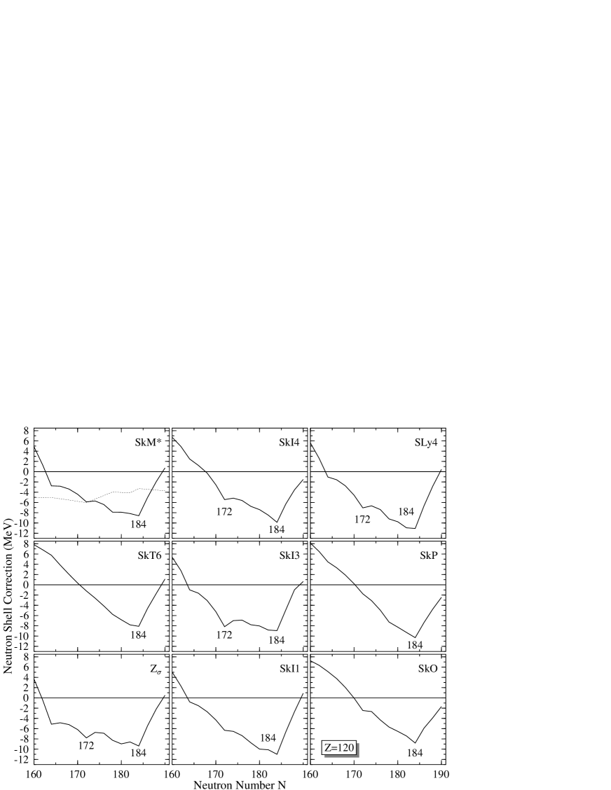
FIG. 3.: Spherical neutron shell corrections for the $Z$=120 isotopes calculated in nine Skyrme-Hartree-Fock models. The dotted line for SkM^∗ shows the proton shell correction for comparison. In all nine cases, the minimum of the shell correction is predicted at $N$=184.

The SHF calculations were carried using the coordinate-space Hartree-Fock code of Ref. [80]. The HF equations were solved by the discretization method. To obtain a proper description of quasi-bound states, it was necessary to take a very large box and a very dense mesh. The actual box size was chosen to be 21 fm and the mesh spacing was 0.3 fm. With this choice, the low-lying positive-energy proton states obtained in SHF perfectly reproduce proton resonances obtained by solving the Schrödinger equation for the HF potential with purely outgoing boundary conditions.

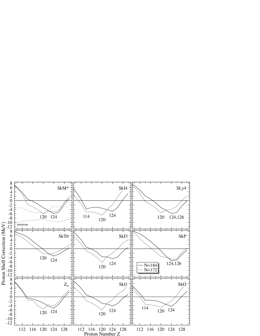
FIG. 4.: Spherical proton shell corrections for the chains of $N$=184 isotones (solid lines) and $N$=172 isotones (dotted lines) calculated in nine Skyrme-Hartree-Fock models. The dashed (dash-dotted) line for SkM$*$ shows the neutron shell correction for $N$=184 ($N$=172). For $N$=184, the minimum of the shell correction is predicted at $Z$=124-126 for all parametrizations.

The Strutinsky procedure contains two free parameters, the smoothing parameter $\gamma$ and the order of the curvature correction $p$. In calculating the Strutinsky smooth energy, instead of the traditional plateau condition we applied the generalized plateau condition described in Ref. [41]. The optimal values of $\gamma$ (in units of oscillator frequency $\hbar\omega_{0}$=41/$A^{1/3}$) calculated for several nuclei turned out to be close to $\gamma_{p}$=1.54 and $\gamma_{n}$=1.66 for protons and neutrons, respectively; these values, together with $p$=10, were adopted in our calculations of shell corrections in SHF.

In the RMF approach, the shell correction can be extracted from the single-particle spectrum like in SHF. To demonstrate it, one proceeds along the steps discussed in Sec. III. The total RMF energy (17) can be decomposed into a smooth part and a correction that fluctuates according to the actual level density. Since the RMF energy functional is bilinear in the densities, the extracted shell correction should be accurate up to order $O(\delta\rho^{2})$.

The RMF calculations were carried out using the coordinate-space code of Ref. [81]. As in the SHF case, the box size was chosen to be 21 fm with a mesh spacing of 0.3 fm.

As already mentioned, all successful RMF parameterizations give a rather small effective mass. This leads to a small level density around the Fermi surface which in turn requires a very large smoothing range $\gamma$ when calculating the smoothed level density $\tilde{g}$. The values for $\gamma$ are strongly correlated with the order of the curvature correction polynomial $p$ [41]; the value $p$=10 chosen here is large enough to provide in nearly all cases a sufficiently smooth $\tilde{g}$, but also small enough that we can restrict the model space to levels up to 60 MeV, which is much larger than the space used in usual RMF calculations. We have adjusted the smoothing range $\gamma$ to the actual level density of a large number of nuclei to fulfill a generalized plateau condition along the strategy of [41]. This leads always to values around $\gamma_{p}$=2.0 for protons and $\gamma_{n}$=2.2 for neutrons. All results presented in this paper are calculated with $p$=10 and $\gamma$ fixed at these values.

VI Results

A Spherical Shell Corrections in Superheavy Nuclei

FIG. 5.: Spherical neutron shell corrections for the $Z$=120 isotopes calculated in six relativistic mean-field models. In all six cases, the minimum of the shell correction is predicted at $N$=172. For NL-Z2 the proton shell correction is given for comparison by the dashed line.

According to the SHF calculations of Ref. [19], the spherical magic neutron number in the SHE region is $N$=184; all the $N$=184 isotones have been predicted to have spherical shapes. The magicity of $N$=184 in SHF is confirmed in this study. Figure 3 displays neutron shell correction calculated in several SHF models as a function of $N$ for $Z$=120. The absolute minimum of shell energy always appears at $N$=184. The $N$=172 shell effect is also seen, but it exhibits a strong force-dependence (it is particularly pronounced for Z_σ, SkI3, SkI4 and SLy4).

As already mentioned, the neutron levels have the same ordering for nearly all forces; all differences seen in the shell corrections are therefore caused by slight changes in the relative distances of the single-particle levels between the models. Forces with large effective masses like SkO, SkP, and SkT6, give a comparatively large level density which washes out the shell effects below $N$=184. Forces with small effective masses (i.e., smaller level density) are much more likely to show significant shell effects at lower neutron numbers around $N$=172.

At fixed $Z$, the proton shell correction changes rather gradually as a function of neutron number; this is illustrated in Fig. 3 for the Skyrme force SkM^∗. (Most of the Skyrme forces give a similar result.) Note that the proton shell corrections are generally smaller than those for the neutrons. At a second glance, however, one sees that the slow variations of the proton shell correction with neutron number are correlated with neutron shell closures. For instance, the $Z$=120 shell correction is largest at neutron numbers around $N$=172 and it becomes reduced when approaching $N$=184. This is caused by the self-consistent rearrangement of single-particle levels according to the actual density distribution in the nucleus and cannot appear in macroscopic-microscopic models with assumed average potentials (see Refs. [30, 31] for more discussion related to this point).

Proton shell corrections for the $N$=184 and $N$=172 isotones, obtained in the SHF model, are displayed in Fig. 4 as a function of $Z$. For SkM^∗, neutron shell corrections are also shown for the $N$=172 and $N$=184 isotones. The shift of the magic proton number with neutron number when going from $N$=172 to $N$=184 is clearly visible. For $N$=172 most of the Skyrme forces (exceptions are SkT6 and SkP) agree on a magic $Z=120$, while for $N=184$ the shell correction shows a minimum at $Z$=124–126 in all cases. (Actually, in most cases, shell-corrections slightly favor $Z$=124 over $Z$=126; this is related to the gradual increase of single-particle energies of 3$p_{3/2}$ and 3$p_{1/2}$ orbitals above $Z$=120.)

Proton shell corrections and the $N$=172 neutron shell corrections are systematically smaller than those for neutrons at $N$=184. This partly explains why spherical ground states of SHE are so well correlated with the magic neutron number $N$=184, see, e.g., [19, 22, 29]. Note that for the majority of Skyrme forces the $N$=172 isotones are predicted to be deformed.

Skyrme forces with non-standard isospin dependence of the spin-orbit interaction are the only ones that give additional (but not very pronounced) shell closures. In the SkI4 model, there appears a secondary minimum at $Z$=114 for $N$=184, while SkI3 is the only Skyrme force which points at $Z$=120 also for $N$=184. A non-standard spin-orbit interaction, however, does not neccesarily lead to shell closures other than $Z$=124-126 for $N$=184. For SkO, which has a spin-orbit force that is similar to SkI4, the $Z$=114 shell is only hinted. It is to be noted that for several interactions such as Z_σ, SkI$x$, and SkO, shell correction changes rather slowly between $Z$=114 and $Z$=126. This indicates that none of the proton shell gaps in this region can be considered as truly “magic”. (The weak $Z$-dependence of proton shell correction above $Z$=114 was pointed out in the early Ref. [82].)

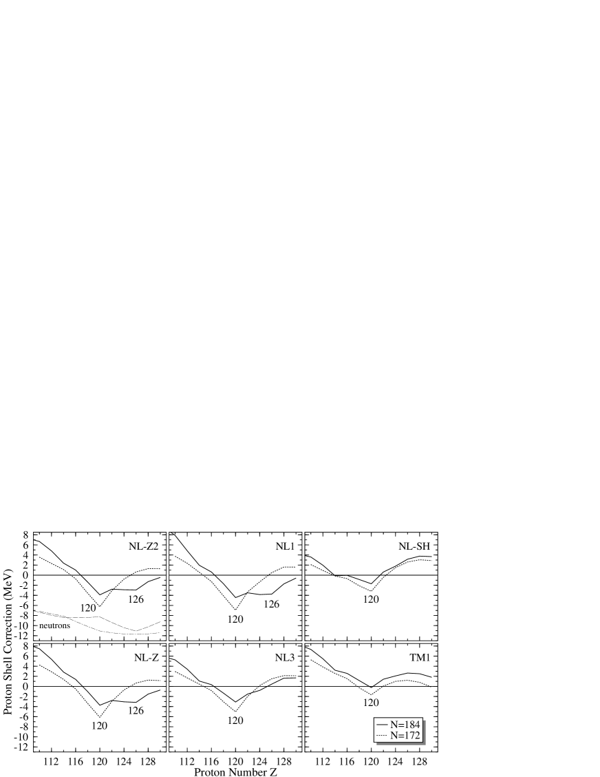
FIG. 6.: Spherical proton shell corrections for the $N$=184 (solid line) and $N$=172 (dotted line) isotones calculated in six relativistic mean-field models. For all parametrizations, the minimum of the proton shell correction is predicted at $Z$=120. For NL-Z2 the neutron shell correction for the $N$=184 (dashed line) and $N$=172 (dash-dotted line) isotones are given for comparison.

The RMF results presented in Figs. 5 and 6 show a pattern that is internally consistent but different from that of SHF. The minimum of neutron shell correction is systematically predicted at $N$=172. Except for NL-SH and TM1, the shell effect at $N$=182-184 is also clearly seen. Note that the $N$=184 gap in the single-particle spectrum is in all cases larger than the one at $N$=182 (see Fig. 2). The gaps are separated by a single $4s_{1/2}$ level which contributes very weakly to the shell energy. To illustrate the variation of proton shell effects along the $Z$=120 chain, proton shell corrections in NL-Z2 are also displayed in Fig. 5. Their pattern is very similar to that obtained in SHF models.

Looking at the proton shell corrections along the chain of $N$=184 isotones, see Fig. 6, the strongest shell effect is now obtained for $Z$=120. When comparing the results for the $N$=184 and $N$=172 chains, it can be seen again that the proton shell correction at $Z$=120 is strongly correlated with neutron number $N$=172. However, unlike in SHF, the $Z$=120 shell does not vanish completely for $N$=184. Proton shell corrections obtained with NL1, NL-Z, and NL-Z2 at $N$=184 vary rather slowly between $Z$=120 and $Z$=126, and this resembles the patterm obtained in SHF. Again, as in the case of Skyrme forces, proton shell corrections in RMF are smaller than those for the neutrons (cf. NL-Z2 calculations in Fig. 6). The increase in the proton shell correction at very large values of $Z$ for TM1 is related to the spherical $Z$=132 shell predicted by this interaction [31].

Shell closures can also be analysed in terms of the two-neutron and two-proton shell gaps

$$\delta_{2n} = E(N+2,Z)-2E(N,Z)+E(N-2,Z),$$ (19)

$$\delta_{2p} = E(N,Z+2)-2E(N,Z)+E(N,Z-2)$$ (20)

discussed in Refs. [31, 77]. The pattern of shell corrections calculated in SHF and RMF nicely follows the behavior of neutron and proton shell gaps found there. In particular, the strong correlation between shell effects at $Z$=120 and $N$=172 in RMF is seen in both representations. While shell gaps are related (but not equivalent) to the gaps in the single-particle spectrum, the shell correction gives also a measure of the stabilizing effect of a shell closure on the nuclear binding energy.

B Macroscopic Energies

By subtracting the shell correction from the calculated binding energy, one obtains a rough estimate for the associated macroscopic energy $E_{\rm macro}$ (9). The macroscopic part of the SHF and RMF energies for the $N$=184 isotones as a function of $Z$ is displayed in Fig. 7. The macroscopic energy of the Yukawa-plus-exponential mass formula of the Finite-Range Liquid Drop Model (FRLDM) of Ref. [20], with parameters of Ref. [21], is also shown for comparison. To illustrate $Z$-dependence, all energies were normalized to the value at $Z$=100. In general, the behavior of $E_{\rm macro}$ is similar in all cases. In particular, the macroscopic proton drip line is consistently predicted to be at $Z$$\approx$120-124. It is interesting to note that the only Skyrme force which agrees with FRLDM is SLy4; other forces deviate from it significantly. The RMF forces give qualitatively the same results; there are several forces (NL-Z, TM1, and NL-SH) which give values of $E_{\rm macro}$ close to the FRLDM.

FIG. 7.: Macroscopic energy $\tilde{E}^{\rm HF}$ (9) extracted from the calculated Hartree-Fock energies of the $N$=184 isotones. For comparison, the phenomenological macroscopic energy of the Yukawa-plus-exponential mass formula (FRLDM) of Ref. [20] with parameters of Ref. [21] is also displayed. To illustrate $Z$-dependence, all energies were normalized to the FRLDM value at $Z$=100.

In an attempt to understand the pattern shown in Fig. 7, we employed the simple liquid drop model expression

$$E_{\rm macro,LDM}=a_{\rm vol}A + a_{\rm surf}A^{2/3}$$ (21)

$$+ a_{\rm sym}\frac{(N-Z)^{2}}{A}+a_{\rm Coul}\frac{Z^{2}}{A^{1/3}}.$$ (22)

The parameters $a_{i}$ of Skyrme and RMF forces were calculated in the limit of symmetric nuclear matter; they are given in Table I, together with the values for the standard liquid drop model (LDM) of Ref. [84]. [Note that these values slightly change when including higher-order terms in the LDM expansion (21).] Figure 8 shows the macroscopic energy (21) as a function of $Z$ for the $N$=184 isotones. The huge differences between results for various Skyrme and RMF parametrizations can be traced back to their different symmetry-energy coefficients. Indeed, for most of the forces discussed, $a_{\rm sym}$ is significantly greater than that of LDM, and this results in an increased slope of $E_{\rm macro,LDM}$. For the RMF forces the significantly larger $a_{\rm vol}$ even further increases the difference with respect to the LDM. Unfortunately, there is very little similarity between the results of microscopic calculations of Fig. 7 and the results of expansion (21). When comparing the energy scales of Figs. 7 and 8, one finds huge differences, of the order of 100 MeV, between $E_{\rm macro}$ and $E_{\rm macro,LDM}$. While for RMF the energy ordering remains the same in both cases, this feature does not hold for SHF. Only when looking at $E_{\rm macro,LDM}$, the results are ordered according to the corresponding values of $a_{\rm sym}$, as expected. All this indicates that even for very heavy nuclei with $A$$\sim$300, the simple leptodermous expansion with parameters taken from nuclear matter calculations is not going to work [85, 86]; the finite-size effects are still very important for SHE.

TABLE I.: Key properties of symmetric nuclear matter for the Skyrme and RMF forces used in this paper: binding energy per nucleon, surface energy, and symmetry energy, all in MeV. The RMF values for $a_{\rm surf}$ are taken from Ref. [83]. The standard liquid drop model (LDM) values [84] are also shown.

Force	$a_{\rm vol}$	$a_{\rm surf}$	$a_{\rm sym}$
SkM∗	$-15.9$	17.59	30.0
Zσ	$-15.9$	16.94	26.7
SkT6	$-16.1$	18.12	29.9
SLy4	$-16.1$	18.18	32.0
SkI1	$-15.9$	17.31	37.5
SkI3	$-16.0$	17.52	34.8
SkI4	$-15.9$	17.28	29.5
SkP	$-16.0$	17.95	30.0
SkO	$-15.8$	17.00	32.0
NL1	$-16.4$	18.66	43.5
NL-Z	$-16.2$	17.72	41.7
NL-Z2	$-16.1$		39.0
NL3	$-16.2$	18.46	37.4
NL-SH	$-16.3$	19.05	36.1
TM1	$-16.3$		36.9
LDM	$-15.7$	18.56	28.1

In spite of the fact that macroscopic energies extracted from different self-consistent models systematically differ, the corresponding shell corrections are similar. For instance, the general pattern and magnitude of shell energies displayed in Figs. 3 and 4 do not depend very much on the Skyrme interaction used, and the same is true for the RMF results shown in Figs. 5 and 6. This means that although the global properties of effective interactions employed in this work differ, their single-particle spectra are fairly similar. Hence, shell corrections extracted from self-consistent single-particle spectra are very useful measures of spectral properties of effective forces. Figure 7 also illustrates how dangerous it is to extrapolate self-consistent results in the region of SHE. The trends of relative binding energies (e.g., $Q_{\alpha}$ values) are expected to smoothly deviate from force to force. The nice agreement with experimental data for the heaviest elements obtained in the SHF calculations with SLy4 [16] and in the macroscopic-microscopic calculations with the FRLDM [21] indicates that the macroscopic energies of forces which are too far off the FRLDM values, i.e. SkM^∗, SkI1, and NL1, are probably not reliable in this region.

FIG. 8.: Macroscopic energy $E_{\rm macro,LDM}$ (21) for the $N$=184 isotones as a function of $Z$ calculated for several Skyrme forces (lines) and the standard liquid drop model (dots). To illustrate the $Z$ dependence, all energies were normalized to zero at $Z$=100. The bulk parameters of Skyrme forces are given in Table I. The Coulomb-energy constant was assumed to be $a_{\rm Coul}$=0.717 MeV [84] in all cases.

Figure 7 shows that the power of a force for predicting total binding energies is fairly independent of its predictive power for shell effects. Forces with a similar (good) description of the smooth trends of binding energies can yield rather different magic numbers; compare, e.g., SLy4 and NL3.

VII Conclusions

The recent experimental progress in the search for new superheavy elements opens a new window for systematic explorations of the limit of nuclear mass and charge. Theoretically, predictions in the region of SHE are bound to be extrapolations from the lighter systems. An interesting and novel feature of SHEs is that the Coulomb interaction can no longer be treated as a small perturbation atop the nuclear mean field; its feedback on the nuclear potential is significant.

The main objective of this study was to perform a detailed analysis of shell effects in SHE. Since many nuclei from this region are close to the proton drip line, a new method of calculating shell corrections, based on the Green’s function approach, had to be developed. This technique was applied to a family of Skyrme interactions and to several RMF parametrizations. This tool turned out to be extremely useful for analyzing the spectral properties of self-consistent mean fields.

It has been concluded that both the SHF and RMF calculations are internally consistent. That is, all the Skyrme models employed in this work predict the strongest spherical shell effect at $N$=184 and $Z$=124,126. On the other hand, all the RMF parametrizations yield the strongest shell effect at $N$=172 and $Z$=120. It is very likely that the main factor contributing to this difference is the spin-orbit interaction, or rather its isospin dependence [30, 59, 62, 63, 64]. The role of the spin-orbit potential in determining the stability of SHE was posed already in the seventies [87, 88]. The experimental determination of the centre of shell stability in the region of SHE will, therefore, be of extreme importance for pinning down the question of the spin-orbit force.

Another interesting conclusion of our work is that the pseudo-spin symmetry seems to be strongly violated in the RMF calculations for SHE. As a matter of fact, the $N$=172 and $Z$=120 magic gaps predicted in the relativistic model appear as a direct consequence of pseudo-spin breaking. This is quite surprising in light of several recent works on the pseudo-spin conservation in RMF [35, 89].

Finally, from calculated masses we extracted self-consistent macroscopic energies. They show a significant spread when extrapolating to unknown SHE. This is expected to give rise to systematic (smooth) deviations between masses and mass differences obtained in various self-consistent models.

- [1] W.D. Myers and W.J. Swiatecki, Nucl. Phys. A81, 1 (1966).
- [2] A. Sobiczewski, F.A. Gareev, and B.N. Kalinkin, Phys. Lett. 22, 500 (1966).
- [3] H. Meldner, Ark. Fys. 36, 593 (1967).
- [4] U. Mosel and W. Greiner, Z. Phys. 222, 261 (1969).
- [5] S. Hofmann and G. Münzenberg, submitted to Rev. Mod. Phys.
- [6] S. Hofmann, Nucl. Phys. A616, 370c (1997).
- [7] S. Hofmann, V. Ninov, F.P. Hessberger, P. Armbruster, H. Folger, G. Münzenberg, H.J. Schött, A.G. Popeko, A.V. Yeremin, A.N. Andreyev, S. Saro, R. Janik, and M. Leino, Z. Phys. A350, 277 (1995); ibid., p. 281.
- [8] A. Ghiorso, D. Lee, L.P. Somerville, W. Loveland, J.M. Nitschke, W. Ghiorso, G.T. Seaborg, P. Wilmarth, R. Leres, A. Wydler, M. Nurmia, K. Gregorich, R. Gaylord, T. Hamilton, N.J. Hannink, D.C. Hoffman, C. Jarzynski, C. Kacher, B. Kadkhodayan, S. Kreek, M. Lane, A. Lyon, M.A. McMahan, M. Neu, T. Sikkeland, W.J. Swiatecki, A. Türler, J.T. Walton, and S. Yashita, Nucl. Phys. A583, 861c (1995).
- [9] Yu.A. Lazarev, Yu.V. Lobanov, Yu.Ts. Oganessian, V.K. Utyonkov, F.Sh. Abdullin, A.N. Polyakov, J. Rigol, I.V. Shirokovsky, Yu.S. Tsyganov, S. Iliev, V.G. Subbotin, A.M. Sukhov, G.V. Buklanov, B.N. Gikal, V.B. Kutner, A.N. Mezentsev, and K. Subotic, J.F. Wild, R.W. Lougheed, and K.J. Moody, Phys. Rev. C54, 620 (1996).
- [10] S. Hofmann, V. Ninov, F.P. Hessberger, P. Armbruster, H. Folger, G. Münzenberg, H.J. Schött, A.G. Popeko, A.V. Yeremin, S. Saro, R. Janik, and M. Leino, Z. Phys. A354, 229 (1996).
- [11] S. Ćwiok and A. Sobiczewski, Z. Phys. A342, 203 (1992).
- [12] R. Smolańczuk, Phys. Rev. C56, 812 (1997).
- [13] R. Smolańczuk, Phys. Rev. C60, 21301 (1999).
- [14] Yu.Ts. Oganessian, A.V. Yeremin, A.G. Popeko, S.L. Bogomolov, G.V. Buklanov, M.L. Chelnokov, V.I. Chepigin, B.N. Gikal, V.A. Gorshkov, G.G. Gulbekian, M.G. Itkis, A.P. Kabachenko, A.Yu. Lavrentev, O.N. Malyshev, J. Rohac, R.N. Sagaidak, S. Hofmann, S. Saro, G. Giargina, and K. Morita, Nature 400, 242 (1999).
- [15] V. Ninov, K.E. Gregorich, W. Loveland, A. Ghiorso, D.C. Hoffman, D.M. Lee, H. Nitsche, W.J. Swiatecki, U.W. Kirbach, C.A. Laue, J.L. Adams, J.B. Patin, D.A. Shaughnessy, D.A. Strellis, and P.A. Wilk, Phys. Rev. Lett. 83, 1104 (1999).
- [16] S. Ćwiok, P.-H. Heenen, and W. Nazarewicz, Phys. Rev. Lett. 83, 1108 (1999).
- [17] M. Bender, submitted to Phys. Rev. Lett.
- [18] S. Åberg, H. Flocard and W. Nazarewicz, Ann. Rev. Nucl. Part. Sci. 40, 439 (1990).
- [19] S. Ćwiok, J. Dobaczewski, P.-H. Heenen, P. Magierski, and W. Nazarewicz, Nucl. Phys. A611, 211 (1996).
- [20] P. Möller and J.R. Nix, At. Data Nucl. Data Tables 39, 213 (1988).
- [21] S. Ćwiok, S. Hofmann, and W. Nazarewicz, Nucl. Phys. A573, 356 (1994).
- [22] G.A. Lalazissis, M.M. Sharma, P. Ring, and Y.K. Gambhir, Nucl. Phys. A608, 202 (1996).
- [23] A. T. Kruppa, Phys. Lett. 431B, 237 (1998).
- [24] S. Ćwiok, V.V. Pashkevich, J. Dudek and W. Nazarewicz, Nucl. Phys. A410 (1983) 254.
- [25] P. Möller and J.R. Nix, J. Phys. G 20, 1681 (1994).
- [26] P. Reiter, T.L. Khoo, C.J. Lister, D. Seweryniak, I. Ahmad, M. Alcorta, M.P. Carpenter, J.A. Cizewski, C.N. Davids, G. Gervais, J.P. Greene, W.F. Henning, R.V.F. Janssens, T. Lauritsen, S.Siem, A.A. Sonzogni, D. Sullivan, J. Uusitalo, I. Wiedenhöver, N. Amzal, P.A. Butler, A.J. Chewter, K.Y. Ding, N. Fotiades, J.D. Fox, P.T. Greenlees, R.-D. Herzberg, G.D. Jones, W. Korten, M. Leino, and K. Vetter, Phys. Rev. Lett. 82, 509 (1999).
- [27] M. Leino, H. Kankaanpaa, R.-D. Herzberg, A.J. Chewter, F.P. Hessberger, Y. Le Coz, F. Becker, P.A. Butler, J.F.C. Cocks, O. Dorvaux, K. Eskola, J. Gerl, P.T. Greenlees, K. Helariutta, M. Houry, G.D. Jones, P. Jones, R. Julin, S. Juutinen, H. Kettunen, T.L. Khoo, A. Kleinbohl, W. Korten, P. Kuusiniemi, R. Lucas, M. Muikku, P. Nieminen, R.D. Page, P. Rahkila, P. Reiter, A. Savelius, Ch. Schlegel, Ch. Theisen, W.H. Trzaska, and H.-J. Wollersheim, Eur. Phys. J. A 6, 63 (1999).
- [28] Z. Patyk and A. Sobiczewski, Nucl. Phys. A533, 132 (1991).
- [29] T. Bürvenich, K. Rutz, M. Bender, P.-G. Reinhard, J.A. Maruhn, and W. Greiner, Eur. Phys. J. A3, 139 (1998).
- [30] M. Bender, K. Rutz, P.-G. Reinhard, J.A. Maruhn, and W. Greiner, Phys. Rev. C60, 34304 (1999).
- [31] K. Rutz, M. Bender, T. Bürvenich, T. Schilling, P.-G. Reinhard, J. A. Maruhn, and W. Greiner, Phys. Rev. C56, 238 (1997).
- [32] A. Arima, M. Harvey, and K. Shimizu, Phys. Lett. 30B, 517 (1969).
- [33] K.T. Hecht and A. Adler, Nucl. Phys. A137, 129 (1969).
- [34] J.N. Ginocchio, Phys. Rev. Lett. 78, 436 (1997).
- [35] J.N. Ginocchio and D.G. Madland, Phys. Rev. C57, 1167 (1998).
- [36] V.M. Strutinsky, Nucl. Phys. A95, 420 (1967).
- [37] V.M. Strutinsky, Nucl. Phys. A122, 1 (1968).
- [38] M. Brack, J. Damgård, A.S. Jensen, H.C. Pauli, V.M. Strutinsky and C. Y. Wong, Rev. Mod. Phys. 44, 320 (1972).
- [39] W. Nazarewicz, T.R. Werner, and J. Dobaczewski, Phys. Rev. C50, 2860 (1994).
- [40] N. Sandulescu, O. Civitarese, R.J. Liotta, and T. Vertse, Phys. Rev. C55, 1250 (1997).
- [41] T. Vertse, A.T. Kruppa, R.J. Liotta, W. Nazarewicz, N. Sandulescu, and T.R. Werner, Phys. Rev. C57, 3089 (1998).
- [42] T. Vertse, K.F. Pál and Z. Balogh, Comp. Phys. Comm. 27, 309 (1982).
- [43] G.G. Bunatian, V.M. Kolomietz and V.V. Strutinsky, Nucl. Phys. A188, 225 (1972).
- [44] M. Brack and P. Quentin, Physics and Chemistry of Fission (IAEA, Vienna, 1974) Vol. I., p. 231.
- [45] P. Ring and P. Schuck, The Nuclear Many-Body Problem (Springer-Verlag, Berlin, 1980).
- [46] M. Brack and P. Quentin, Nucl. Phys. A361, 35 (1981).
- [47] M. Brack and P. Quentin, Phys. Lett. 56B, 421 (1975).
- [48] M. Bolsterli, E.O. Fiset, J.R. Nix, and J.L. Norton, Phys. Rev. C5, 1050 (1972).
- [49] R. Balian and C. Bloch, Ann. Phys. (NY) 60, 401 (1970).
- [50] R. Balian and C. Bloch, Ann. Phys. (NY) 69 (1971) 76.
- [51] S. Shlomo, Nucl. Phys. A539, 17 (1992).
- [52] S. Shlomo, V.M. Kolomietz, and H. Dejbakhsh, Phys. Rev. C55, 1972 (1996).
- [53] P. Quentin and H. Flocard, Annu. Rev. Nucl. Part. Sci. 28, 523 (1978).
- [54] J. Bartel, P. Quentin, M. Brack, C. Guet, and H.B. Håkansson, Nucl. Phys. A386, 79 (1982).
- [55] F. Tondeur, M. Brack, M. Farine, and J.M. Pearson, Nucl. Phys. A420, 297 (1984).
- [56] J. Friedrich and P.-G. Reinhard, Phys. Rev. C33, 335 (1986).
- [57] J. Dobaczewski, H. Flocard, and J. Treiner, Nucl. Phys. A422, 103 (1984).
- [58] E. Chabanat, Interactions effectives pour des conditions extrêmes d’isospin, Université Claude Bernard Lyon-1, Thesis 1995, LYCEN T 9501, unpublished.
- [59] P.-G. Reinhard and H. Flocard, Nucl. Phys. A584, 467 (1995).
- [60] P.-G. Reinhard, D.J. Dean, W. Nazarewicz, J. Dobaczewski, J.A. Maruhn, and M.R. Strayer, Phys. Rev. C60, 014316 (1999).
- [61] D. Vautherin and D.M. Brink, Phys. Rev. C5, 626 (1972).
- [62] M.M. Sharma, G. Lalazissis, G. König, and P. Ring, Phys. Rev. Lett. 74, 3744 (1995).
- [63] E. Chabanat, P. Bonche, P. Haensel, J. Meyer, and F. Schaeffer, Physica Scripta T56, 231 (1995).
- [64] M. Onsi, R.C. Nayak, J.M. Pearson, H. Freyer, W. Stocker, Phys. Rev. C55, 3166 (1997).
- [65] P.-G. Reinhard, Rep. Prog. Phys. 52, 439 (1989).
- [66] C. Speicher, R.M. Dreizler, and E. Engel, Ann. Phys. (N.Y.) 213, 312 (1992).
- [67] R.N. Schmid, E. Engel, and R.M. Dreizler, Phys. Rev. C52, 164 (1995).
- [68] R.N. Schmid, E. Engel, and R.M. Dreizler, Phys. Rev. C52, 2804 (1995).
- [69] R.N. Schmid, E. Engel, and R.M. Dreizler, Foundations of Physics 27, 1257 (1997).
- [70] M. Bender, K. Rutz, P.-G. Reinhard, and J. A. Maruhn, Eur. Phys. J. A, in press.
- [71] P.-G. Reinhard, M. Rufa, J. Maruhn, W. Greiner, and J. Friedrich, Z. Phys. A323, 13 (1986).
- [72] M. Rufa, P.-G. Reinhard, J. A. Maruhn, W. Greiner, and M. R. Strayer, Phys. Rev. C 38, 390 (1988).
- [73] M.M. Sharma, M.A. Nagarajan, and P. Ring, Phys. Lett. B312, 377 (1993).
- [74] G.A. Lalazissis, J. König, and P. Ring, Phys. Rev. C55, 540 (1997).
- [75] Y. Sugahara and H. Toki, Nucl. Phys. A579, 557 (1994).
- [76] G.A. Lalazissis, M.M. Sharma, P. Ring, and Y.K. Gambhir, Nucl. Phys. A608, 202 (1996).
- [77] M. Bender, K. Rutz, P.-G. Reinhard, J. A. Maruhn, and W. Greiner, Proceedings of Nuclear Shapes and Motions, A Symposium in Honor of Ray Nix, Santa Fe, New Mexico, October 25–27, 1998. Acta Physica Hungarica N. S. Heavy-Ion Physics, in press.
- [78] P.-G. Reinhard, Z. Phys. A329, 257 (1988).
- [79] M. Bender, K. Rutz, P.-G. Reinhard, J.A. Maruhn, and W. Greiner, Phys. Rev. C58, 2126 (1998).
- [80] P.-G. Reinhard, in Computational Nuclear Physics I Eds. K. Langanke, S.E. Koonin, and J.A. Maruhn, (Springer Verlag, Berlin, 1991) p.28.
- [81] K. Rutz, Struktur von Atomkernen im Relativistic-Mean-Field Modell, Ph. D. Thesis, J. W. Goethe-Universtität Frankfurt am Main, (Ibidem-Verlag, Stuttgart, 1999).
- [82] M. Bolsterli, E.O. Fiset, J.R. Nix, and J.L. Norton, Phys. Rev. Lett. 27, 681 (1971).
- [83] W. Stocker and T.v. Chossy, Phys. Rev. C58, 2777 (1998).
- [84] W.D. Myers and W.J. Swiatecki, Ann. Phys. (N.Y.) 55, 395 (1969).
- [85] M. Brack, C. Guet, and H.-B. Håkansson, Phys. Rep. 123, 275 (1985).
- [86] M. Brack and R.K. Bhaduri, Semiclassical Physics (Addison-Wesley, Reading, Mass., 1997).
- [87] J.M. Moss, Phys. Rev. C17, 813 (1978).
- [88] Y. Tanaka, Y. Oda, F. Petrovich, and R.K. Sheline, Phys. Lett. 83B, 279 (1979).
- [89] J. Meng, K. Sugawara-Tanabe, S. Yamaji, P. Ring, and A. Arima, Phys. Rev. C58, R628 (1998).