Nuclear Matter on a Lattice

Abstract

We investigate nuclear matter on a cubic lattice. An exact thermal formalism is applied to nucleons with a Hamiltonian that accommodates on-site and next-neighbor parts of the central, spin- and isospin-exchange interactions. We describe the nuclear matter Monte Carlo methods which contain elements from shell model Monte Carlo methods and from numerical simulations of the Hubbard model. We show that energy and basic saturation properties of nuclear matter can be reproduced. Evidence of a first-order phase transition from an uncorrelated Fermi gas to a clustered system is observed by computing mechanical and thermodynamical quantities such as compressibility, heat capacity, entropy and grand potential. We compare symmetry energy and first sound velocities with literature and find reasonable agreement.

I Introduction

Properties of nuclear matter have been deduced from different approaches. The volume term of the semi-empirical mass formula [1, 2] predicts a binding energy of $16\;{\rm MeV}$, and calculations of finite nuclei estimate the equilibrium density to be $\rho_{0}=0.16\;{\rm fm^{-3}}$. However, properties of finite nuclei are strongly influenced by finite size effects like the surface effect, and it is therefore difficult to estimate energies and saturation density of nuclear matter from nuclei. Many-body calculations of nuclear matter are based on sophisticated potentials (such as the Argonne AV14 and AV18 and Urbana UV14 potentials) and use Bethe-Brueckner-Goldstone theory [3, 4, 5] and hypernetted chain approximations [6, 7] to calculate ground state properties. Lattice gas calculations [8, 9, 10] attempt a thermal description of nuclear matter. They work with much simpler Hamiltonians, incorporating isospin-1 or Hubbard-like interactions. These calculations aim at the investigation of a liquid-gas phase transition of nuclear matter expected to take place at subnuclear densities and low temperatures. They are classical, not quantum mechanical, putting in kinetic terms by hand or sampling them from a Maxwell-Boltzmann distribution. These types of calculations use Monte-Carlo-like algorithms and show that the inclusion of a kinetic term is crucial to observe a phase transition.

This paper describes first results of a calculation of infinite nuclear matter that combines both the usage of a more realistic Hamiltonian and the exact, thermal treatment of the many-body problem on a lattice. In the last few years, the shell model Monte Carlo (SMMC) method has been successfully developed [11, 12, 13, 14, 15] to give a powerful alternative to direct diagonalization procedures which suffer from the fact that the many-body space scales so unfavorably with the number of single-body states considered. Direct diagonalization methods can only address very light nuclei or nuclei with a closed shell and only a few valence nucleons. The SMMC avoids this combinatorial scaling (in storage and computation time) and makes it possible to investigate structural properties of nuclei far beyond the few-nucleon system. The SMMC enforces the Pauli-principle exactly, and concentrates on the evaluation of thermal averages of observables. This would be the main purpose of a nuclear matter investigation too: Not focusing on obtaining a wave function, a thermal formalism is useful for a study of nuclear matter, because the equation of state is of main interest, which clearly depends on density and temperature. Moreover, the consideration of a large piece of infinite nuclear matter in coordinate space reduces finite size effects that appear after imposing periodic boundary conditions. A formalism written in momentum space has the disadvantage that two- or many-body correlations cannot be calculated directly: Clustering (and therefore a possible liquid-gas transition) is not as easily calculated and observed as in the coordinate space representation.

The following concept is pursued for our nuclear matter calculation: The quantum mechanical and exact treatment with the full Hamiltonian, kinetic and potential term, should be a prerequisite for a successful description of the physical system. In a coordinate representation nucleons shall interact with a potential that eventually comes as close to a realistic nuclear interaction (like AV18) as possible. The partition function along with observables of interest shall be calculated in the grand canonical ensemble, in order to control temperature $T$ and density $\rho$. The latter is to be adjusted on average via the chemical potential $\mu$. The many-body problem shall be solved exactly using Monte Carlo methods similar to those used in the SMMC applications. At the same time, realizing that the emerging equations eventually have to be solved on a computer, one should take into account that space will be discretized, and advantage should be taken of the available technology that has been employed for the Hubbard and other models in condensed matter physics. This paper is to be viewed as a first step of a full thermal description of nuclear matter in which we constrain our potential parameters to a reasonable shape of the energy as a function of density, including the correct saturation point.

II Theory of Nucleonic Matter on a Lattice

The general concept of the nuclear matter calculation consists of nucleons interacting via a variety of components of the nuclear two-body potential. While it should be the ultimate goal to use a potential that fits the nucleon-nucleon scattering data best [16], at the first stage we concentrate on few parts of the interactions, namely central, spin- and isospin-exchange. The degrees of freedom of the nucleon are its spin, isospin as well as the spatial coordinate.

Subnuclear degrees of freedom are not explicitly incorporated. The lightest meson, the pion, facilitates an interaction with a range of $r\approx 1.4\;{\rm fm}$ which is of same order as the lattice spacing of the applications in this paper. Since the system is ultimately regularized on a lattice, the argument can be made that all subnuclear degrees of freedom are integrated out, resulting in a strong on-site and weaker next-neighbor interaction. The lattice spacing, here an additional fitting parameter like the potential parameters, is chosen to be of $a=1.842\;{\rm fm}$. This particular lattice spacing sets the half-filling of the lattice at $\rho=2\rho_{0}=0.32\;{\rm fm^{-3}}$. Other settings of fillings have been tried, but turned out to reproduce the saturation curve less well.

In this section we specify the Hamiltonian of the system and describe the nuclear matter Monte Carlo method (called NMMC hereafter), which consists of the thermal formalism to express the grand canonical partition function as an integral over single-body evolution operators. At its center stands the Hubbard-Stratonovitch transformation, which is used to reduce the many-body problem to an effective one-body problem. The details of the Monte Carlo procedure, which is used to evaluate the resulting multi-dimensional integral, are explained.

A Hamiltonian

We consider a three-dimensional cubic lattice of spacing $a$ and assume periodic boundary conditions, which result in a three-dimensional toroidal configuration. The coordinate $\vec{x}$ and the momentum $\vec{p}$ are discretized as

$$\vec{x}\rightarrow a\vec{m}\equiv\vec{x}_{m},$$ (1)

$$\vec{p}\rightarrow\left(\frac{2\pi}{Na}\right)\vec{k}\equiv\vec{p}_{k},$$ (2)

such that

$$\vec{x}\cdot\vec{p}=\frac{2\pi}{N}\times{\rm integer},$$ (3)

where $N$ is the number of lattice points in each spatial direction, and $\vec{m}$ and $\vec{k}$ are vectors with integer components.

The nucleons have mass $m_{N}$, spin $\sigma=\pm\frac{1}{2}$ and isospin $\tau=\pm\frac{1}{2}$ . The Hamiltonian,

$$\hat{\cal H}=\hat{\cal K}+\hat{\cal V},$$ (4)

is expressed in second quantization and contains kinetic and potential operators. The kinetic term is written as

$$\hat{\cal K}=-\frac{\hbar^{2}}{2m_{N}}\sum_{\sigma\tau}\int{\rm d}\vec{x}\;\psi^{\dagger}_{\sigma\tau}(\vec{x})\vec{\nabla}^{2}\psi_{\sigma\tau}(\vec{x}).$$ (5)

The fermion operator $\psi^{\dagger}_{\sigma\tau}(\vec{x})$ creates a nucleon of spin and isospin $(\sigma,\tau)$ at location $\vec{x}$, while its adjoint $\psi_{\sigma\tau}(\vec{x})$ destroys it. This equation is discretized on the lattice by the symmetric 3-point formula for the second derivative, and the integral is replaced by a finite sum, which results in

$$\hat{\cal K}=-t_{0}\sum_{\sigma\tau}a^{3}\sum_{\vec{x}_{n},i=1\cdots 3}\psi^{\dagger}_{\sigma\tau}(\vec{x}_{n})\left[\psi_{\sigma\tau}(\vec{x}_{n}+a\vec{e}_{i})-2\psi_{\sigma\tau}(\vec{x}_{n})+\psi_{\sigma\tau}(\vec{x}_{n}-a\vec{e}_{i})\right]$$ (6)

with

$$t_{0}=\frac{\hbar^{2}}{2m_{N}a^{2}}.$$ (7)

Here, the orthogonal unit vectors $\{\vec{e}_{i}\}$ span the three-dimensional space.

While the form of the nuclear potential is generally given, we here are limited by current computational constraints. The treatment of a full Hamiltonian, as it is represented in the Argonne potential, for example, is computationally impossible with currently available computer power, but may be feasible in a few years. We chose

$$\hat{\cal V}=\hat{\cal V}_{c}+\hat{\cal V}_{\sigma}.$$ (8)

The first part is the central potential ($\hat{\cal V}_{c}$), followed by the spin-exchange ($\hat{\cal V}_{\sigma}$). The general form for the scalar potential,

$$\hat{\cal V}_{c}=\frac{1}{2}\sum_{\sigma\tau\sigma^{\prime}\tau^{\prime}}\int{\rm d}\vec{x}\;\int{\rm d}\vec{x}^{\prime}\;\psi^{\dagger}_{\sigma\tau}(\vec{x})\psi^{\dagger}_{\sigma^{\prime}\tau^{\prime}}(\vec{x}^{\prime})V_{c}(\vec{x}-\vec{x}^{\prime})\psi_{\sigma^{\prime}\tau^{\prime}}(\vec{x}^{\prime})\psi_{\sigma\tau}(\vec{x}),$$ (9)

can be written in terms of the density

$$\hat{\rho}(\vec{x})=\sum_{\sigma\tau}\hat{\rho}_{\sigma\tau}(\vec{x})=\sum_{\sigma\tau}\psi^{\dagger}_{\sigma\tau}(\vec{x})\psi_{\sigma\tau}(\vec{x}).$$ (10)

The purpose of doing so is to cast the potential in linear and quadratic terms, as the Hubbard-Stratonovitch transformation can only be performed on quadratic terms. Using the fermion anticommutation relation, the potential then becomes

$$\hat{\cal V}_{c}=\frac{1}{2}\int{\rm d}\vec{x}\;\int{\rm d}\vec{x}^{\prime}\;V_{c}(\vec{x}-\vec{x}^{\prime})\hat{\rho}(\vec{x})\hat{\rho}(\vec{x}^{\prime})-\frac{1}{2}\int{\rm d}\vec{x}\;V_{c}(0)\hat{\rho}(\vec{x}).$$ (11)

The last term is the self-energy and is a consequence of the Pauli principle. The discretized version of this equation is

$$\hat{\cal V}_{c}=\frac{a^{6}}{2}\sum_{\vec{x}_{n},\vec{x}^{\prime}_{n}}V_{c}(\vec{x}_{n}-\vec{x}^{\prime}_{n})\hat{\rho}(\vec{x}_{n})\hat{\rho}(\vec{x}^{\prime}_{n})-\frac{a^{3}}{2}\sum_{\vec{x}_{n}}V_{c}(0)\hat{\rho}(\vec{x}_{n}).$$ (12)

We assume a Skyrme-like on-site and next-neighbor interaction

$$V_{c}\left(\vec{x}_{n}-\vec{x}^{\prime}_{n}\right)=V^{(0)}_{c}\delta\left(\vec{x}_{n}-\vec{x}^{\prime}_{n}\right)+V^{(2)}_{c}\left(\nabla^{2}_{\vec{x}_{n}}\delta\left(\vec{x}_{n}-\vec{x}^{\prime}_{n}\right)\right),$$ (13)

whose discretized form is

$$V_{c}(\vec{x}_{n}-\vec{x}^{\prime}_{n})=\frac{V^{(0)}_{c}}{a^{3}}\delta_{\vec{x}_{n},\vec{x}^{\prime}_{n}}+\frac{V^{(2)}_{c}}{a^{5}}\sum_{i=1}^{3}\left\{\delta_{\vec{x}_{n}+a\vec{e}_{i},\vec{x}^{\prime}_{n}}-2\delta_{\vec{x}_{n},\vec{x}^{\prime}_{n}}+\delta_{\vec{x}_{n}-a\vec{e}_{i},\vec{x}^{\prime}_{n}}\right\}.$$ (14)

The parentheses in Eq. (13) indicate that the Laplace operator only acts on the $\delta$-function, but not on any following parts. Inserting equation (14) into (12) gives

$$\hat{\cal V}_{c}=\frac{V^{(0)}_{c}}{2}\sum_{\vec{x}_{n}}a^{3}\hat{\rho}(\vec{x}_{n})^{2} - \frac{V^{(2)}_{c}a}{2}\sum_{\vec{x}_{n}}\sum_{i=1}^{3}\left(\hat{\rho}\left(\vec{x}_{n}+a\vec{e}_{i}\right)-\hat{\rho}\left(\vec{x}_{n}\right)\right)^{2}$$ (15)

$$- \frac{1}{2}\left(V^{(0)}_{c}-6\frac{V^{(2)}_{c}}{a^{2}}\right)\sum_{\vec{x}_{n}}\hat{\rho}(\vec{x}_{n}),$$ (16)

Here, we applied periodic boundary conditions.

The spin-exchange part of the potential is handled in a very similar way. Starting from

$$\hat{\cal V}_{\sigma}=\frac{1}{2}\sum_{{\xi\tau\xi^{\prime}\tau^{\prime}}\atop{\kappa\lambda\kappa^{\prime}\lambda^{\prime}}}\int{\rm d}\vec{x}\;\int{\rm d}\vec{x}^{\prime}\;\psi^{\dagger}_{\xi\tau}(\vec{x})\psi^{\dagger}_{\xi^{\prime}\tau^{\prime}}(\vec{x}^{\prime})V_{\sigma}(\vec{x}-\vec{x}^{\prime})\vec{\bf\sigma}_{\xi\tau\kappa\lambda}\cdot\vec{\bf\sigma}_{\xi^{\prime}\tau^{\prime}\kappa^{\prime}\lambda^{\prime}}\psi_{\kappa^{\prime}\lambda^{\prime}}(\vec{x}^{\prime})\psi_{\kappa\lambda}(\vec{x}),$$ (17)

we write the potential in form of spin densities

$$\hat{\rho}^{(\alpha)}_{\sigma}(\vec{x})=\sum_{\xi\tau\kappa\lambda}\psi^{\dagger}_{\xi\tau}(\vec{x}){\bf\sigma}^{(\alpha)}_{\xi\tau\kappa\lambda}\psi_{\kappa\lambda}(\vec{x}),\;\alpha=0,+,-,$$ (18)

where ${\bf\sigma}^{(\alpha)}_{\xi\tau\kappa\lambda}$ are the elements of a generalized Pauli spin-isospin matrix, which acts on a 4-vector representing all spin/isospin states of a nucleon. We assume the the same spatial dependence (13) as for the central part, and finally arrive at

$$\hat{\cal V}_{\sigma} = \frac{V^{(0)}_{\sigma}}{2}\sum_{\vec{x}_{n}}a^{3}\left(\hat{\rho}^{(0)}_{\sigma}\left(\vec{x}_{n}\right)^{2}+2\left(\hat{\rho}^{(+)}_{\sigma}\left(\vec{x}_{n}\right)+\hat{\rho}^{(-)}_{\sigma}\left(\vec{x}_{n}\right)\right)^{2}\right)$$ (19)

$$- \frac{V^{(2)}_{\sigma}a}{2}\sum_{\vec{x}_{n}}\sum_{i=1}^{3}\left(\left(\hat{\rho}^{(0)}_{\sigma}(\vec{x}_{n}+a\vec{e}_{i})-\hat{\rho}^{(0)}_{\sigma}(\vec{x}_{n})\right)^{2}\right.$$ (20)

$$+ \left.2\left(\hat{\rho}^{(+)}_{\sigma}\left(\vec{x}_{n}+a\vec{e}_{i}\right)+\hat{\rho}^{(-)}_{\sigma}\left(\vec{x}_{n}+a\vec{e}_{i}\right)-\hat{\rho}^{(+)}_{\sigma}\left(\vec{x}_{n}\right)-\hat{\rho}^{(-)}_{\sigma}\left(\vec{x}_{n}\right)\right)^{2}\right)$$ (21)

$$- \frac{3}{2}\left(V^{(0)}_{\sigma}-6\frac{V^{(2)}_{\sigma}}{a^{2}}\right)\sum_{\vec{x}_{n}}\hat{\rho}\left(\vec{x}_{n}\right).$$ (22)

Other components of the potential can be included in a similar way.

B Nuclear Matter Monte Carlo Method

In order to study thermal properties of nuclear matter, the grand canonical partition function at a given temperature $T=\beta^{-1}$ needs to be determined,

$$Z={\rm\hat{Tr}}\left[\exp\left(-\beta\left(\hat{\cal H}-\sum_{\sigma\tau}\mu_{\tau}\hat{\cal N}_{\sigma\tau}\right)\right)\right]\equiv{\rm\hat{Tr}}\left[\hat{U}\right],$$ (23)

with $\hat{\cal N}_{\sigma\tau}=\sum_{\vec{x}_{n}}\psi^{\dagger}_{\sigma\tau}(\vec{x}_{n})\psi_{\sigma\tau}(\vec{x}_{n})$ and $\mu_{\tau}$ as the isospin-dependent chemical potential. $\hat{U}$ is called the imaginary-time evolution operator of the system and is a many-body operator. In the present study the Hamiltonian $\hat{\cal H}$ contains one- and two-body operators as described Section II A, and the trace is taken over all many-body states as indicated by a caret. The partition function $Z$ is an exponential over all one- and two-body operators (and therefore interactions) present in the system. It is impossible to deal with the partition function $Z$ in this form, because the number of many-body correlations that have to be kept track of grows rapidly with system size. We therefore seek an expression for $Z$ that is based on a single-particle representation, and we will replace the many-body problem with that of non-interacting nucleons that are coupled to a heat bath of auxiliary fields. This involves rewriting $Z$ as a multi-dimensional integral.

We start by dividing the evolution operator into $n_{t}$ time slices:

$$\hat{U}=\exp\left(-\beta\left(\hat{\cal H}-\sum_{\sigma,\tau}\mu_{\tau}\hat{\cal N}_{\sigma\tau}\right)\right)=\left[\exp\left(-\Delta\beta\left(\hat{\cal H}-\sum_{\sigma,\tau}\mu_{\tau}\hat{\cal N}_{\sigma\tau}\right)\right)\right]^{n_{t}},$$ (24)

with $\Delta\beta n_{t}=\beta$. The Trotter approximation [17, 18] is used to separate one-body (kinetic energy and chemical potential) in $\hat{\cal S}\equiv\hat{\cal K}-\sum_{\sigma,\tau}\mu_{\tau}\hat{\cal N}_{\sigma\tau}$ and two-body terms (potential) in $\hat{\cal H}$:

$$\exp\left(-\Delta\beta\left(\hat{\cal H}-\sum_{\sigma,\tau}\mu_{\tau}\hat{\cal N}_{\sigma\tau}\right)\right)=\exp\left(-\Delta\beta\left(\hat{\cal S}+\hat{\cal V}\right)\right)\approx\exp\left(-\Delta\beta\hat{\cal S}\right)\exp\left(-\Delta\beta\hat{\cal V}\right).$$ (25)

Equation (25) is valid to order $\Delta\beta$, but becomes exact in the limit $\Delta\beta\rightarrow 0$.

The propagator of each time slice for the potential, $\exp(-\Delta\beta\hat{\cal V})$, is manipulated by applying the Hubbard-Stratonovitch (HS) transformation [19, 20] on each term, replacing it with a multi-dimensional integral over a set of auxiliary fields.

As an example, we describe the transformation by taking the on-site part of $\hat{\cal V}_{c}$ at one particular site $\vec{x}_{m}$. Using $\alpha\equiv\Delta\beta V^{(0)}_{c}/2$ and defining

$$S_{\alpha}=\left\{\begin{array}[]{ll}\pm i&{\rm if}\;\alpha>0\\ \pm 1&{\rm if}\;\alpha<0,\end{array}\right.$$ (26)

the propagator for this single interaction is written as

$$\Delta\hat{U}\left(\vec{x}_{m}\right) \equiv \exp\left(-\Delta\beta\frac{V^{(0)}_{c}}{2}\hat{\rho}^{2}\left(\vec{x}_{m}\right)\right)=\sqrt{\frac{|\alpha|}{\pi}}\int_{-\infty}^{\infty}{\rm d}\chi\exp\left(-\alpha\hat{\rho}^{2}\left(\vec{x}_{m}\right)-|\alpha|\left(\chi+S_{\alpha}\hat{\rho}\left(\vec{x}_{m}\right)\right)^{2}\right)$$ (27)

$$= \sqrt{\frac{|\alpha|}{\pi}}\int_{-\infty}^{\infty}{\rm d}\chi\exp\left(-|\alpha|\left[\chi^{2}+2S_{\alpha}\chi\hat{\rho}\left(\vec{x}_{m}\right)\right]\right).$$ (28)

The last line of Eq. (27) reveals that the evolution operator is now expressed in terms of the exponential of a one-body operator and an integration over the auxiliary field $\chi$. It has become a one-body propagator that corresponds to non-interacting nucleons coupled to this field. Since the integral is calculated with Monte Carlo methods, the field fluctuates according to a weight that is to be specified, hence the picture of a heat bath.

It has to be emphasized that $\hat{\rho}\left(\vec{x}_{m}\right)$ here represents a one-body operator for a subset ($\hat{\cal V}_{c}$ in this case) of the full interaction. Each quadratic term in (15) and (19) has to be replaced by an integral. At a given lattice site $\vec{x}_{m}$, there are twelve auxiliary fields to form the full interaction, four for $\hat{\cal V}_{c}$ and eight for $\hat{\cal V}_{\sigma}$. Nucleons are now coupled to a big ensemble of auxiliary fields through which the interaction of the nucleons is mediated. The $\Delta\hat{U}$’s are then multiplied together to form the evolution operator for one time slice $\hat{U}\left(\beta_{m}\right)$ at $\beta_{m}=m\Delta\beta$, which is expressed only in terms of single-body matrices, and ultimately, all time slices are multiplied together to form $\hat{U}$:

$$\hat{U}=\left[\exp\left(-\Delta\beta\hat{\cal H}\right)\right]^{n_{t}}=\int{\cal D}\left[\chi\right]G\left(\chi\right)\hat{U}_{\chi}\left(\beta,0\right)$$ (29)

with the integration measure

$${\cal D}\left[\chi\right]=\prod_{m=1}^{n_{t}}\prod_{\vec{x}_{n}}\prod_{i}{\rm d\chi}_{m,\vec{x}_{n},i}\sqrt{\frac{|\alpha_{i}|}{\pi}}.$$ (30)

The $\alpha_{i}=\Delta\beta V_{i}/2,\;V_{i}\in\left[V^{(0)}_{c},V^{(2)}_{c},V^{(0)}_{\sigma},\cdots\right]$, are the interaction-specific coupling strengths of auxiliary fields to nucleons, and the index $i$ enumerates all fields at a particular site. The Gaussian factor $G$ is given by

$$G\left(\chi\right)=\prod_{m=1}^{n_{t}}\prod_{\vec{x}_{n}}\prod_{i}\exp\left(-|\alpha_{i}|\chi^{2}_{m,\vec{x}_{n},i}\right),$$ (31)

and the one-body propagator is

$$\hat{U}_{\chi}\left(\beta,0\right)=\hat{U}\left(\beta_{n_{t}}\right)\hat{U}\left(\beta_{n_{t}-1}\right)\cdots\hat{U}\left(\beta_{1}\right).$$ (32)

Note that Eq. (29) only becomes exact in the limit of an infinite number of time slices, $n_{t}\rightarrow\infty$. For a finite $n_{t}$, the Hubbard-Stratonovitch approximation is valid only to order $\Delta\beta$.

In the practical implementation of Eq. (27), a discrete Hubbard-Stratonovitch transformation is used instead of the continuous form because it turns out to use much fewer de-correlation sweeps, as explained below.

A thermal observable $\langle\hat{O}\rangle$ is expressed as [12, 21]

$$\langle\hat{O}\rangle=\frac{1}{Z}{\rm\hat{Tr}}\left[\hat{O}\exp\left(-\beta\left(\hat{{\cal H}}-\sum_{\sigma,\tau}\mu_{\tau}\hat{\cal N}_{\sigma\tau}\right)\right)\right]=\frac{\int{\cal D}[\chi]G(\chi)\langle\hat{O}(\chi)\rangle\xi(\chi)}{\int{\cal D}[\chi]G(\chi)\xi(\chi)}$$ (33)

and has the integration measure of Eq. (30) and Gaussian factor of Eq. (31). The expectation value of any operator in second quantization can be obtained with the help of Wick’s theorem, and the resulting one-body densities are [12]

$$\langle\psi^{\dagger}_{\sigma\tau}\left(\vec{x}_{n}\right)\psi_{\sigma^{\prime}\tau^{\prime}}\left(\vec{x}_{m}\right)\rangle_{\chi}=\left\{\left[{\bf 1}+{\bf U}_{\chi}\left(\beta,0\right)\right]^{-1}{\bf U}_{\chi}\left(\beta,0\right)\right\}_{(\sigma^{\prime}\tau^{\prime},\vec{x}_{m}),(\sigma\tau,\vec{x}_{n})}.$$ (34)

The bold face ${\bf U}_{\chi}\left(\beta,0\right)$ is the single-body matrix representation of $\hat{U}_{\chi}\left(\beta,0\right)$. Observables of the system are chosen to be the number of neutrons and protons and all components of the energy.

The integrals in (33) are evaluated using the Metropolis algorithm [22]. The basic idea involves sampling the integrand of (33),

$$\langle\hat{O}(\chi)\rangle=\frac{\hat{\rm Tr}\left[\hat{O}\hat{U}_{\chi}\left(\beta,0\right)\right]}{\hat{\rm Tr}\left[\hat{U}_{\chi}\left(\beta,0\right)\right]},$$ (35)

within the boundaries of the integration volume according to a positive-definite weight

$$W\left(\chi\right)=\left\{\begin{array}[]{ll}|G(\chi)\xi(\chi)|&{\rm for\;continuous\;HS}\\ |\xi(\chi)|&{\rm for\;discrete\;HS},\end{array}\right.$$ (36)

with

$$\xi(\chi)=\hat{\rm Tr}\left[\hat{U}_{\chi}\left(\beta,0\right)\right]=\det\left[{\bf 1}+{\bf U_{\chi}}\left(\beta,0\right)\right].$$ (37)

The last equality can be proven by expanding the determinant [21]. Samples are taken by a random walker that travels through $\chi$-space, taking a new value $\chi_{\rm new}$ from the previous one $\chi_{\rm old}$ if the ratio

$$r=\frac{W(\chi_{\rm new})}{W(\chi_{\rm old})}$$ (38)

is larger than one, or else, if $r<1$, taking on $\chi_{\rm new}$ with probability $r$. It can be shown [23] that the sequence of values the walker takes is distributed according to the weight function $W\left(\chi\right)$, which is typically chosen to be as close to the integrand as possible to increase the efficiency of the procedure. Since the consecutive steps are correlated, the walker has to travel several steps before another sample is taken to de-correlate them. The average of an observable (33) is then simply

$$\langle\hat{O}\rangle=\frac{\sum_{i}\langle\hat{\cal O}\rangle_{i}\Phi_{i}}{\sum_{i}\Phi_{i}}$$ (39)

in terms of its $i$th Monte Carlo sample $\langle\hat{\cal O}\rangle_{i}$ and

$$\Phi=\left\{\begin{array}[]{ll}\frac{G(\chi)\xi(\chi)}{W\left(\chi\right)}&{\rm for\;continuous\;HS}\\ \frac{\xi(\chi)}{W\left(\chi\right)}&{\rm for\;discrete\;HS}.\end{array}\right.$$ (40)

Note that $\Phi$, which is just the sign of the weight $W$, can generally be negative or even complex.

The numerical determination of Eq. (39), which is the Monte Carlo equivalent of the integrals in Eq. (33), can be difficult in certain situations, even with Monte Carlo methods: If $S_{\alpha}=\pm i$ (which generally corresponds to a repulsive on-site and an attractive next-neighbor interaction, cf. Eq. (26)), propagators for the potential (Eq. (27)) contribute negative or complex elements to $\hat{U}_{\chi}\left(\beta,0\right)$ (see Eq. (37)). The integrands in both numerator and denominator are oscillatory, and the integrals can add up to small numbers. A numerical evaluation with Monte Carlo methods causes large uncertainties because the methods are of a stochastic nature, and the number of samples in a computation remains finite. This is a complication associated with these methods when the Hubbard-Stratonovitch transformation is used. It is referred to as the Monte Carlo sign problem. A pragmatic solution has been used for the shell model Monte Carlo method to handle this complication [15].

There has been significant effort in stabilizing and optimizing the Metropolis algorithm for lattice calculations, as they have been heavily used for models of interacting electrons in condensed matter physics. Many of the techniques have directly been applied to NMMC, because the models are similar. Besides using the checkerboard breakup [21] technique for kinetic and spin-exchange parts, we use the Green’s function algorithm described in [25] to reduce the computational burden.

III Numerical Results

We now show that for symmetric nuclear matter (SNM) the energy per particle can be reproduced quite well over a wide range of densities, and the energy for pure neutron matter (PNM) for the same potential is discussed. Then, several observations are presented that give evidence of a first-order phase transition from a Fermi gas to a clustered system at a critical temperature $T_{c}\sim 15\;{\rm MeV}$. Furthermore, the symmetry energy and first sound are discussed.

The extensive search in the space of potential parameters included all components of the central part and spin-exchange. The effort focused on reproducing saturation density and energy correctly. The project is considered to be a first step towards a realistic calculation as indicated earlier. A more realistic calculation has to contain more parts of the nuclear potential and the spatial resolution has to improve; a perfect fit over a wide range of densities should not be expected at this point. The fit has been performed in such a manner that the saturation energy and density is reproduced, and that the overall energy curve has a reasonable form: for sub-saturation densities, the matter should be unstable, while for $\rho>\rho_{0}$ SNM should evolve in an unbound state ($E/A>0\;{\rm MeV}$ for $\rho\geq 0.4\;{\rm fm^{-3}}$).

The sign problem unfortunately forces the use of a nuclear potential that might contradict the usual physical understanding and intuition based on few-nucleon potential models. It is generally known that the central potential has a strong repulsion for short distances and features a long-range attraction. Here, the desire to avoid the sign problem generates the opposite: on-site attraction and next-neighbor repulsion. On the other hand, an on-site attraction and next-neighbor repulsion may not be unreasonable given the fact that there have been several mean-field calculations of nuclear matter with the Skyrme forces. Skyrme forces simulate the interaction with a $\delta$-like attraction and a $\nabla^{2}\delta$-like repulsion. In the lattice discretization of this investigation, the position of the nucleons at the same site is only determined up to a cube of size $a$. Therefore, the on-site potential parameter can be seen as an average potential within that cube, and by tuning the lattice spacing accordingly, it could be possible that this parameter is negative. The exact definition of the parameter depends on a regularization scheme. In such a scheme the Schrödinger equation has to be solved on a lattice, and by identifying scattering amplitudes, one could determine the potential parameters from scattering lengths and effective range [24]. With respect to the lattice spacing $a$ two approaches can be taken: First, we constrain ourselves to a description with a fixed number of lattice sites. Then $a$ becomes a free fitting parameter like the potential parameters, and the latter would have to be interpreted as an average potential, as noted above. In the second approach, $a$ is an discretization parameter for the potential, and the ultimate goal would be to increase the number of lattice points with decreasing $a$, getting a smooth parameterization of the potential. If, in that case, a positive on-site parameter is used, emulating a hard core repulsion, one has to deal with oscillatory integrands and commensurately large error bars.

The following potential parameters were obtained:

$$V_{c}^{(0)} = -181.5\;{\rm MeV\,fm^{3}},$$ (41)

$$V_{c}^{(2)} = 37.8\;{\rm MeV\,fm^{5}},$$ (42)

$$V_{\sigma}^{(0)} = -31.25\;{\rm MeV\,fm^{3}},$$ (43)

$$V_{\sigma}^{(2)} = 0.0\;{\rm MeV\,fm^{5}}.$$ (44)

All calculations were done with this set of parameters. The lattice has a spacing of

$$a=1.842\;{\rm fm},$$ (45)

tuned such that quarter filling of the lattice is at saturation density $\rho_{0}=0.16\;{\rm fm^{-3}}$. In this paper, the lattice spacing is an additional fitting parameter, and several other settings have been tested. However, quarter- and half-filling at saturation density have a special significance because certain lattice occupations of the nucleons result in an energetically favored configuration.

Because of limited CPU time, the calculation is restricted to $4\times 4\times 4$ lattices for the moment. This lattice comprises $10^{38}$ many-body states, and 11520 auxiliary fields are used for this set of parameters. All calculations are prepared by a pre-thermalization of the system for 100 steps before we took measurement samples. Between measurement samples, 15 de-correlation steps have been taken to guarantee statistical independence of the samples. The autocorrelation of $k$ consecutive samples [23]

$$C_{\cal{O}}\left(k\right)=\frac{\langle{\cal{O}}_{i}{\cal{O}}_{i+k}\rangle-\langle{\cal{O}}_{i}\rangle^{2}}{\langle{\cal{O}}_{i}^{2}\rangle-\langle{\cal{O}}_{i}\rangle^{2}},$$ (46)

with $i$ being the summation index over samples, has been monitored for all observables $\cal{O}$ and was held below $10\%$.

We are also restricted by the fact that the Monte Carlo simulations cannot be extended to arbitrarily low temperatures. Even though the numerical routines are quite stable, it is not possible to add an arbitrary number of time slices, since it involves more and more matrix multiplications which become increasingly numerically unstable. In the present case we take $\Delta\beta=0.01\;{\rm MeV^{-1}}$ and were able to go down to a value of $\beta=30\times\Delta\beta=0.3\;{\rm MeV^{-1}}$ without running into numerical instabilities. Thus, the temperature range of the investigation is

$$3.0\;{\rm MeV}\leq T\leq 100\;{\rm MeV}.$$ (47)

Fig. 1 shows the best fit we obtained. With decreasing temperature, the system develops a minimum at $\rho=0.32\;{\rm fm^{-3}}$ first, which is most pronounced between $10-14\;{\rm MeV}$, before it shifts to lower densities. At $T=3.3\;{\rm MeV}$ and $T=5.9\;{\rm MeV}$ the minimum is very broad, making matter softer (see also compressibility, Fig. 4 below). For high temperatures and/or high density, the simulation suffers from the fact that it runs out of model space: At $T=50\;{\rm MeV}$ the system behaves almost like a Fermi gas and the energy per particle should behave like $\sim\rho^{2/3}$. Yet, the curve bends down. Also, for all other temperatures, the curves converges to the energy of the full lattice state, $E/A=5.96\;{\rm MeV}$, as density increases. For sub-saturation densities the model gives more binding if compared to other calculations (see, for example, Refs. [6] and [7]), and the energy is not as high for densities beyond saturation. At $\rho=0.32\;{\rm fm^{-3}}$, $E/A$ as a function of temperature has a minimum at $T\approx 10\;{\rm MeV}$ which means that at even lower temperatures $E/A$ increases again. This contradicts intuition because it would mean that the system is in an unphysical state.

The last issue needs further explanation. The energy per particle is not the correct quantity in order to address the question of stability. Particles fluctuate in and out of the system differently at different temperature, leaving the average number of particles unchanged, but contributing to the two-body part of the Hamiltonian. If, however, the grand potential is plotted (see Fig. 2),

$$\Omega\left(\beta,\mu\right)=-T\ln{\cal{Z}}\left(\beta,\mu\right),$$ (48)

with

$$\ln{\cal{Z}}\left(\beta,\mu\right)-\ln{\cal{Z}}\left(0,\mu\right)=-\int_{0}^{\beta}{\rm d}\beta^{\prime}E\left(\beta^{\prime},\mu\right),$$ (49)

it turns out to actually be a monotonic function of temperature, with a slight deviation at $\mu=11.0\;{\rm MeV}$ where the negative slope of $\Omega$, the entropy

$$S=-\left(\frac{\partial\Omega}{\partial T}\right)_{\mu,V},$$ (50)

becomes zero between $10\;{\rm MeV}$ and $14\;{\rm MeV}$ and positive again for even lower temperatures. This is a slight anomaly (see also Fig. 5) which may have been caused by the onset of numerical instabilities at low temperatures or the fact that the lattice spacing is so big and the number of sites so small that the discretization of space is not accurate enough.

We now introduce several observations which indicate that the system may undergo a first-order phase transition towards a clustered system when the temperature is lowered. First, we investigate changes in density with respect to the chemical potential $\mu$. It is well known that they are proportional to particle fluctuations

$$\sigma^{2}_{N}=T\left.\frac{\partial\langle N\rangle}{\partial\mu}\right|_{T,V}\sim\left.T\frac{\partial\rho}{\partial\mu}\right|_{T,V}.$$ (51)

Such fluctuations are typical for first-order phase transitions and indicate that particles move between the two phases without energy cost. For an infinite system, the fluctuations should diverge, but not for a finite system. In the present case, we expect particles building clusters and breaking them up again, so one phase — the gas phase — would be that of independent particles, the other one that of clusters. Since we observe the single particle density, $\sigma^{2}_{N}$ describes the fluctuations in the gas phase in which $\rho$ is linear in $\mu$. At $T=100\;{\rm MeV}$, we are in the gas phase with nucleons behaving like a Fermi gas. Therefore, to simplify the graphs, we have first fitted the data at $T=100\;{\rm MeV}$ to a linear function,

$$\rho_{\rm fit}=a_{\scriptscriptstyle\rm fit}+b_{\scriptscriptstyle\rm fit}\times\mu,$$ (52)

and then subtracted this function from all data points of all temperatures, defining a function of temperature and chemical potential

$$f\left(T,\mu\right)=\rho\left(T,\mu\right)-\rho_{\rm fit}.$$ (53)

The upper panel of Fig. 3 shows the outcome of this procedure. We then take the derivative of $f\left(T,\mu\right)$ with respect to $\mu$ and multiply with $T$, and this is shown in the lower panel of Fig. 3. The fluctuations show a pronounced maximum for $T=14.3\;{\rm MeV}$ and $\mu\approx-8\;{\rm MeV}$, while they are low for $T=3.3\;{\rm MeV}$ and $T=100\;{\rm MeV}$. The phase transition seems to occur somewhere between $T=8\;{\rm MeV}$ and $T=20\;{\rm MeV}$.

Another quantity that suggests the existence of a transition is the compressibility which is given by

$$\kappa=9\rho^{2}\left.\frac{\partial^{2}E/A}{\partial\rho^{2}}\right|_{\rho=\rho_{\rm sat}},$$ (54)

where $\rho_{\rm sat}$ is the saturation density. We have fitted the minima of each energy curve to a quadratic function

$$\left.\frac{E}{A}\right|_{\rm fit}\left(\rho\right)=a+b\times\left(\rho-\rho_{\rm sat}\right)^{2},$$ (55)

and determined the compressibility as $\kappa=18\rho_{\rm sat}^{2}\times b$. All data points in Fig. 4 were obtained with a $\chi^{2}$ per degree of freedom of less than $1.5$. Again, a maximum in compressibility (which is in fact an incompressibility) is observed at $T\approx 14\;{\rm MeV}$: The clusters that form repel each other through the next-neighbor interaction which is repulsive. At $T<14\;{\rm MeV}$, matter becomes softer again due to a broadening of the minima in $E/A$. This can be explained if one assumes that the system becomes more dilute. Note that the values of $\rho_{\rm sat}$ change with temperature.

Finally, we present the heat capacity and entropy of the system. For a first-order phase transition, the continuous and infinite system shows a divergence in the heat capacity

$$c_{V}=\left.\frac{\partial E}{\partial T}\right|_{V},$$ (56)

and a discontinuity for the entropy (with an infinite derivative at $T_{c}$),

$$S\left(\beta,\mu\right)=\ln{\cal{Z}}+\beta\langle H\left(\beta,\mu\right)\rangle-\beta\mu\langle N\left(\beta,\mu\right)\rangle.$$ (57)

For a finite system only a maximum in the heat capacity is expected, and a relatively sharp drop in entropy with decreasing temperature. Both facts can be verified in Fig. 5: The heat capacity suggests a critical temperature of $T_{c}=15\;{\rm MeV}$, as does the entropy. For the graphs of entropy one has to keep in mind that the system investigated is quite small (it is a $4\times 4\times 4$ lattice only), but two levels, $S\approx 75$ from $T=5\;{\rm MeV}$ to $T=12\;{\rm MeV}$ and $S=175$ from $T=20\;{\rm MeV}$ to $T=30\;{\rm MeV}$ with a steep decrease in between, can definitely be identified. To show that this is indeed a first-order phase transition, the calculation has to be repeated for a larger number of lattice sites, and then it has to be demonstrated that the drop between the two levels becomes steeper and steeper, finally resulting in a step-like function. This will have to be left for a future project. Studies of a lattice gas model [26] have shown that finite size effects do induce anomalies in physical quantities, and a first-order phase transition rather appears as a second-order one. The anomaly below $T=10\;{\rm MeV}$ has been addressed when discussing the grand potential. However, the latter quantity shows a qualitative behaviour at $\mu=11\;{\rm MeV}$ that is expected for a phase transition (cf Fig. 2). The infinite system has a kink (the derivative is not continuous) in the grand potential at the critical temperature. Consequently, all quantities consistently suggest a phase transition at a critical temperature of $T_{c}\approx 15\;{\rm MeV}$.

In Fig. 6 we show the energy per particle for pure neutron matter. The uncertainties for this case are much larger than for symmetrical nuclear matter. As a potential, we used the parameters obtained from the fit to symmetric nuclear matter, even though we could have fitted the potential parameters for this case anew, including an isospin-exchange potential. Therefore we view the results for pure neutron matter more as a test to see how well the given potential already reproduces the energy. Note that the slopes of the curves at high temperatures are not negative as it is for symmetrical nuclear matter. But clearly, we cannot conclude that the energies at $T=3.3\;{\rm MeV}$ have converged to that of the ground state because the curve differs quite a bit from that of $T=5.9\;{\rm MeV}$. At the lowest temperature they are $4-5\;{\rm MeV}$ higher than those of the ground state as calculated in Ref. [6], but the general shape of the curve is very similar. This is no surprise, since pure neutron matter is like a Fermi gas, with attractive forces between neutrons lowering the energies with respect to the non-interacting system. The search for any kind of phase transition in the range of $5-50\;{\rm MeV}$ was to no avail. It is likely that a phase transition occurs at lower temperature.

We finally calculate two additional observables and compare them with other calculations found in the literature. The symmetry energy, which appears as a coefficient $a_{sym}$ in the semi-empirical mass formula

$$\frac{E_{sym}}{A}=a_{sym}\frac{\left(N-Z\right)^{2}}{A^{2}},$$ (58)

is plotted in Fig. 7. We used the energy per particle of pure neutron matter (PNM) and SNM, subtracted them and interpolated the result on a mesh. Since the error bars for pure neutron matter are larger for low temperatures, the graphs should be viewed with caution. Nevertheless it appears that the symmetry energy is increasing with density and decreasing with temperature, as one would expect. Indeed, at high temperature SNM and PNM both are more like a Fermi gas, and only at low temperatures do they become different. The observed dependence on density can be explained by the fact that a dilute system is barely interacting while the probability of clustering increases with density. At saturation density and low temperature, we obtain a coefficient of

$$a_{sym}\approx 38\pm 3\;{\rm MeV},$$ (59)

which is not too different from the generally accepted value [27] of $a_{sym}=28.1\;{\rm MeV}$. This discrepancy is in part due to the fact that the calculations for pure neutron matter have not converged completely.

The first sound velocity has been calculated using the formalism of relativistic fluid dynamics:

$$u/c=\sqrt{\left.\frac{\partial p}{\partial e}\right|_{S}},$$ (60)

where

$$e=\rho\times\left(m_{N}c^{2}+\frac{E}{A}\right)$$ (61)

and

$$p=\rho^{2}\left.\frac{\partial E/A}{\partial\rho}\right|_{S}.$$ (62)

In general, the first sound we obtain is too low compared to Ref. [6, 28], but the velocities are of the same order of magnitude. Several calculations [6, 28] show a violation of causality at a few multiples of the saturation density, and so do ours. Our results (Fig. 8) show the correct temperature dependence in the sense that it conforms with the compressibility: higher sound speed for intermediate temperatures (high incompressibility) and lower speeds for both low and high $T$.

IV Discussion and Conclusion

The model considered in this paper is an exact treatment taking first steps towards a more realistic Hamiltonian, and it is an improvement compared to previous calculations. Nevertheless it can be extended to include more physics, and details in the algorithm can be improved. First of all, more computer power is necessary to reduce finite size effects. A lattice of $10\times 10\times 10$ points would be desirable, and also the imaginary time dimension could be pushed further. This requires stable matrix techniques. The present code can handle 30 time slices comfortably using commonly known sparse matrix techniques. But, as the lattice spacing decreases, one needs to go to larger imaginary time to separate the ground state from excited states. At the same time it is not possible to increase $\Delta\beta$ as it would induce finite time effects. Therefore, an improved effective matrix algorithm would be needed to allow for more matrices to be multiplied. Along with a bigger lattice, the resolution of the potential could be increased, resulting in next-to-nearest-neighbor and further interactions. This extension of the spatial dependence of the potential can easily be accomplished and is only restricted by computational power.

Another big hurdle is the sign problem. The solution to this obstacle will result in a huge advancement in many areas of computational physics and chemistry. Rom et al. [29] have made some progress which could prove beneficial for the model described here too: It basically consists of shifting the contour of the auxiliary field integrals, which is equivalent to subtracting a mean-field from the problem. We plan to investigate this method and its application to nuclear matter more rigorously in the future.

The physics of nuclear matter itself is certainly more involved than the current model can account for. Mesons are not included as explicit degree of freedom, and the various exchanges are only simulated indirectly through the choice of potential and its parameters, very much like in AV18 or other potentials. Realizing that the auxiliary fields behave like massless bosons, one could ponder how a Monte Carlo procedure would look like that includes meson exchange directly. Such a procedure could be quite similar to already established auxiliary field Monte Carlo procedures.

It is known that three-body and perhaps higher-order many-body forces are important to describe saturation properties of nuclear matter correctly. However, incorporating these forces in a Monte Carlo calculation is currently impossible, basically because there is no scheme to reduce higher-order forces to the single particle formalism. Such a scheme could lie in a multiple application of the Hubbard-Stratonovitch transformation for a single many-body interaction. But as long as such a scheme is not available, an approximation could be established on top of this two-body calculation that incorporates higher-order effects. A first attempt would be to calculate the three-body contribution to the energy obtained from the one-body densities of this Monte Carlo calculation and a given three-body Hamiltonian.

In conclusion, this project has produced promising results which should be viewed as a starting point to an exact solution of infinite nuclear matter. In a model with a relatively simple Hamiltonian, and further limited by a very small lattice, we were able to reproduce saturation properties of symmetric nuclear matter. The energy of pure neutron matter, using the same potential, gave reasonable results, even though it had not yet converged. Furthermore, we presented evidence in form of mechanical and thermodynamical observables which support the existence of a phase transition from a Fermi gas to a clustered system. Particle fluctuations of the gas phase seem to reach a maximum at $T\approx 14\;{\rm MeV}$. The heat capacity and compressibility also have a maximum at around this temperature. Entropy and grand potential show a behaviour as it is expected for a first-order phase transition. Other quantities like symmetry energy and first sound velocity show reasonable agreement with other calculations.

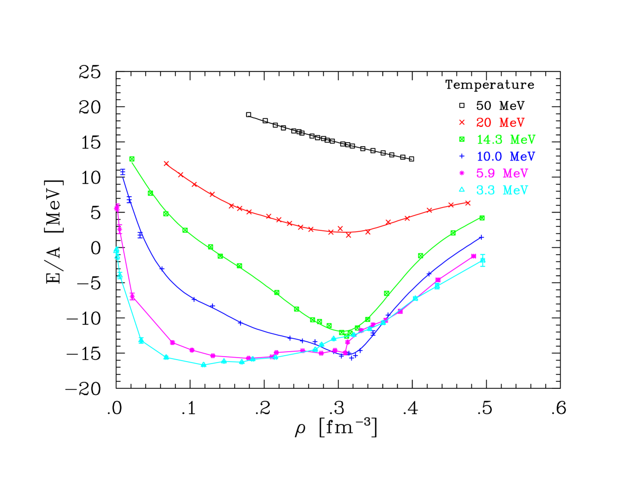
FIG. 1.: $E/A$ for symmetric nuclear matter as a function of density $\rho$ and for different temperatures. The purpose of the lines is to guide the eye.

FIG. 2.: Grand canonical potential of symmetric nuclear matter for different chemical potentials $\mu$. The solid lines represent the potential for a noninteracting Fermi gas in continuous space.

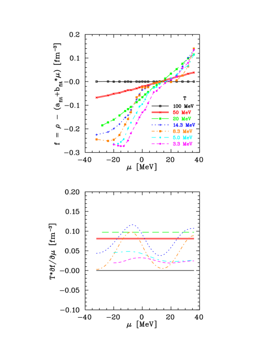
FIG. 3.: Density fluctuations in symmetric nuclear matter. The upper panel displays the modified density $f$ while the lower panel shows the derivatives of $f$ with respect to chemical potential $\mu$ which are proportional to the fluctuations.

FIG. 4.: Compressibility of symmetric nuclear matter. The minima of the energy curves have been fit to a parabola with a $\chi^{2}\leq 1.5$ per degree of freedom.

FIG. 5.: Heat capacity and entropy for a finite piece of symmetrical nuclear matter. The two graphs on the left show the case $\mu=0.0\;{\rm MeV}$, the right ones for $\mu=4.0\;{\rm MeV}$. The heat capacity (upper panels) shows a distinct maximum, the entropy (lower panels) a relatively sharp drop with decreasing temperatures.

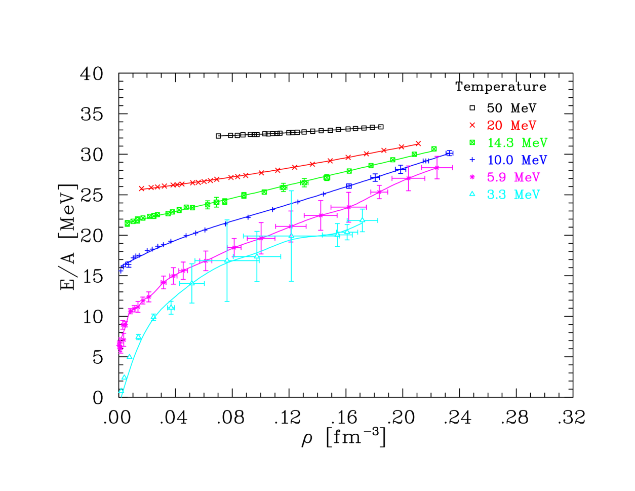
FIG. 6.: $E/A$ for pure neutron matter as a function of density $\rho$ and for different temperatures. The lines guide the eye.

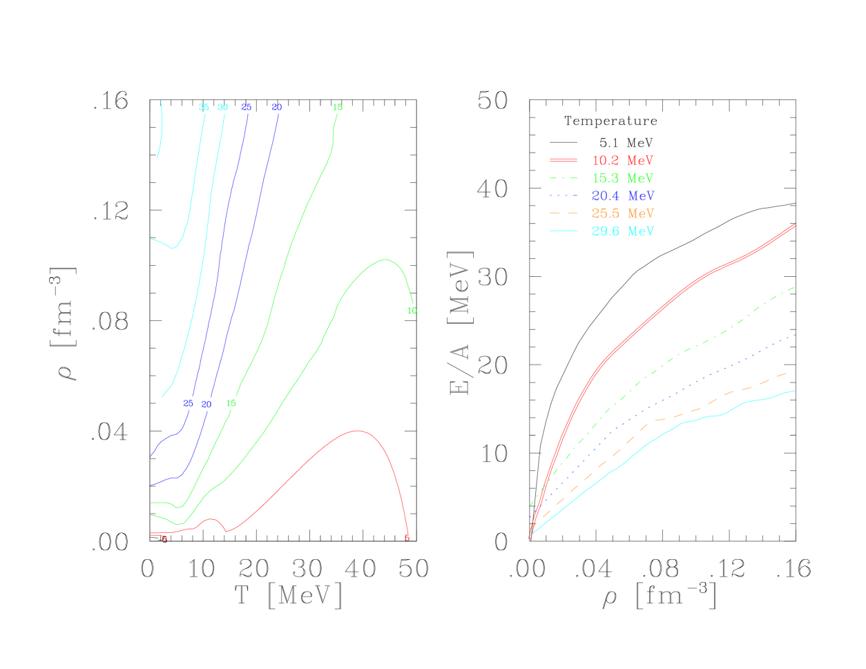
FIG. 7.: Symmetry energy for symmetric nuclear matter as a function of density and temperature. Shown is the coefficient $a_{sym}$ of the semi-empirical mass formula. The left panel shows a contour plot, the right one shows one-dimensional cross-sections of it at different temperatures. $a_{sym}$ is increasing with density and decreasing with temperature.

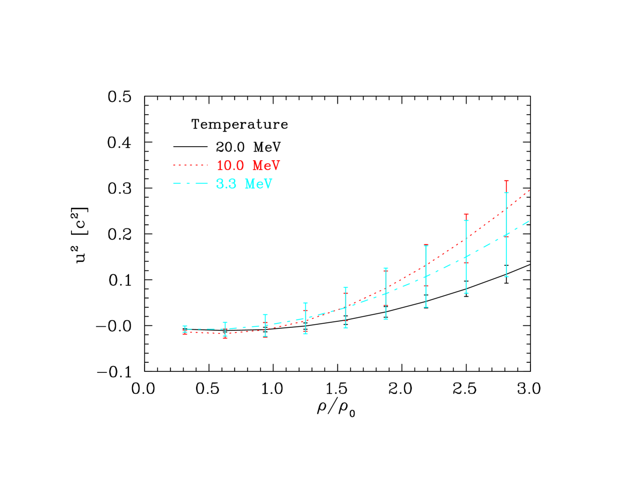
FIG. 8.: First sound velocity for symmetric nuclear matter. The temperature dependence of the speed corresponds to the compressibilities as shown in Fig. 4.

- [1] C.F. von Weizsäcker, Z. Phys. 96, 431 (1935).
- [2] H.A. Bethe and R.F. Bacher, Rev. Mod. Phys. 8, 82 (1936).
- [3] K.A. Brueckner, Phys. Rev. 97, 1353 (1955).
- [4] H.A Bethe and J. Goldstone, Proc. Roy. Soc. (London) A238, 551 (1957).
- [5] J. Goldstone, Proc. Roy. Soc. (London) A239, 267 (1957).
- [6] R.B. Wiringa, V. Fiks and A. Fabrocini, Phys. Rev. C 38, 1010 (1988).
- [7] A. Akmal and V.R. Pandharipande, Phys. Rev. C 56, 2261 (1997).
- [8] T.T.S. Kuo, S. Ray, J. Shamanna, and R.K. Su, Int. J. Mod. Phys. E 5, 303 (1996).
- [9] X. Campi and H. Krivine, Nucl. Phys. A 620, 46 (1997).
- [10] J. Pan and S. Das Gupta, Phys. Rev. C 57, 1839 (1998).
- [11] C.W. Johnson, S.E. Koonin, G.H. Lang, and W.E. Ormand, Phys. Rev. Lett. 69, 3157 (1992).
- [12] G.H. Lang, C.W. Johnson, S.E. Koonin, and W.E. Ormand, Phys. Rev. C 48, 1518 (1993).
- [13] W.E. Ormand, D.J. Dean, C.W. Johnson, and S.E. Koonin, Phys. Rev. C 49, 1422 (1994).
- [14] Y. Alhassid, D.J. Dean, S.E. Koonin, G.H. Lang, and W.E. Ormand, Phys. Rev. Lett. 72, 613 (1994).
- [15] S.E. Koonin, D.J. Dean, and K. Langanke, Phys. Rep. 278, 1 (1997).
- [16] R.B. Wiringa, V.G.J. Stoks, and R. Schiavilla, Phys. Rev. C 51, 38 (1995).
- [17] H.F. Trotter, Proc. Am. Math. Soc. 10, 545 (1959).
- [18] M. Suzuki, Commun. Math. Phys. 51, 183 (1976).
- [19] J. Hubbard, Phys. Lett. 3, 77 (1959).
- [20] R.D. Stratonovitch, Dokl. Akad. Nauk. SSSR 115, 1907 (1957).
- [21] E.Y Loh, Jr. and J.E. Gubernatis, in Electronic Phase Transitions, edited by W. Hanke and Yu.V. Kopaev, Elsevier Science Publishers B.V., New York, 1992.
- [22] N. Metropolis, A.W. Rosenbluth, M.N. Rosenbluth, A.H. Teller, and E. Teller, J. Chem. Phys. 21, 1087 (1953).
- [23] S.E. Koonin and D.C. Meredith, Computational Physics, Addison-Wesley Publishing Company, Reading, 1990.
- [24] H.-M. Müller and R. Seki, in Nuclear Physics with Effective Field Theory, edited by R. Seki, U. van Kolck, and M.J. Savage, World Scientific Publishing Co. Pte. Ltd., Singapore, 1998.
- [25] S.R. White, D.J. Scalapino, R.L. Sugar, E.Y. Loh, J.E. Gubernatis, and R.T. Scalettar, Phys. Rev. B 40, 506 (1989).
- [26] F. Gulminelli and P. Chomaz, Phys. Rev. Lett. 82, 1402 (1999).
- [27] P. Ring and P. Schuck, The Nuclear Many-Body Problem, Springer-Verlag, Heidelberg, 1980, p 4.
- [28] E. Osnes and D. Strottman, Phys. Lett. 166B, 5 (1986).
- [29] N. Rom, D.M. Charutz, and D. Neuhauser, Chem. Phys. Lett. 270, 382 (1997).