ELECTRON SCATTERING WITH A
SHORT-RANGE CORRELATION MODEL

Abstract

The inclusive electromagnetic responses in the quasi–elastic region are calculated with a model which considers the terms of the cluster expansion containing a single correlation line. The validity of this model is studied by comparing, in nuclear matter, its results with those of a complete calculation. Results in finite nuclei for both one– and two–nucleon emission are presented.

I Introduction

Aim of the nuclear many–body theories is the calculation of the properties of finite nuclear systems by having as only input the bare nucleon–nucleon interaction. The approach we follow to solve the nuclear many–body problem is based upon the variational principle

$$\delta E[\Psi_{0}]=\delta\frac{\langle\Psi_{0}|H|\Psi_{0}\rangle}{\langle\Psi_{0}|\Psi_{0}\rangle}=0\,\,.$$ (1)

The solution of eq. (1) is exactly that of the Schrödinger equation if there are no limitations on the Hilbert space spanned to search for the minimum of the energy functional. In our approach we search for the minimum within a subspace composed by states of the form

$$|\Psi_{0}\rangle=F|\Phi_{0}\rangle\,\,\,,$$ (2)

where $|\Phi_{0}\rangle$ is a Slater determinant, formed by a set of orthonormal single particle wave functions, and $F$ is a many–body correlation function.

The quantities to be compared to the experiment are calculated by evaluating the mean value of the corresponding operators between the states of eq. (2) fixed at the minimum of the energy functional:

$$\langle Q\rangle=\frac{\langle\Phi_{0}|F^{+}QF|\Phi_{0}\rangle}{\langle\Phi_{0}|F^{+}F|\Phi_{0}\rangle}\,\,\,,$$ (3)

where we have indicated with $Q$ a generic operator associated to an observable.

A good variational ansatz for realistic calculations requires that the correlation function $F$ has the same operatorial dependence of the Hamiltonian. In this report, however, we assume that the many–body correlation is a scalar function which can be written as a product of two-body correlation functions:

$$F({\bf r}_{1},{\bf r}_{2},....,{\bf r}_{A},)=\prod_{i<j}^{A}f({r_{ij})}$$ (4)

where $r_{ij}$ is the distance between the nucleons $i$ and $j$. The choice (4) of the correlation function leads to the following expression for the energy functional:

$$E[F\Phi_{0}] = \frac{\langle\Phi_{0}|H\prod_{i<j}^{A}f^{2}(r_{ij})|\Phi_{0}\rangle}{\langle\Phi_{0}|\prod_{i<j}^{A}f^{2}(r_{ij})|\Phi_{0}\rangle}$$ (5)

$$= \frac{\langle\Phi_{0}|H[1+h(r_{12})][1+h(r_{13})].....[1+h(r_{23})]...|\Phi_{0}\rangle}{\langle\Phi_{0}|[1+h(r_{12})][1+h(r_{13})].....[1+h(r_{23})]...|\Phi_{0}\rangle}$$ (6)

In the above equation we have used the function $h(r_{ij})=f^{2}(r_{ij})-1$ to show the mechanism of the cluster expansion.

The simplest term is the mean value of the hamiltonian between two uncorrelated states, which is obtained by picking up all the “ones” in the various terms in eq. (6). More complicated terms are obtained considering a single $h(r_{ij})$ function multiplying the “ones”. The procedure continues considering terms with two, three, etc. $h(r_{ij})$ functions. We make a classification of the various terms based upon their topology. With the Fermi Hypernetted Chain (FHNC) technology we calculate all the terms of a certain type. Details of the application of the FHNC to the description of the ground state of doubly closed shell nuclei can be found in refs. [1]$-$[4]. The recent progresses of these calculations, done with state dependent correlations, are presented in another contribution to this conference [5].

II The model: ground state

In the theoretical framework we have presented, the evaluation of an operator mean value, eq. (3), requires the use of the full FHNC computational scheme. For the evaluation of the one–body density distribution, defined as

$$\rho({\bf r}_{1})=\frac{A}{\langle\Psi_{0}|\Psi_{0}\rangle}\int d^{3}r_{2}.....\int d^{3}r_{A}\Psi_{0}^{*}({\bf r}_{1},....,{\bf r}_{A})\Psi_{0}({\bf r}_{1},....,{\bf r}_{A})\,\,,$$ (7)

we have developed a simplified model [6, 7]. After performing the cluster expansion of both numerator and denominator to eliminate the so-called unlinked diagrams, we retain the terms with a single correlation function $h$. The expression for the density obtained in this approximation is:

$$\rho_{1}({\bf r}_{1})=\int d^{3}r_{2}.....\int d^{3}r_{A}$$ (8)

$$\Phi_{0}^{*}({\bf r}_{1},....,{\bf r}_{A})\left[1+\sum_{i=2}^{A}h(r_{1i})+\sum_{i=2}^{A}\sum_{j>i}^{A}h(r_{ij})\right]_{L}\Phi_{0}({\bf r}_{1},....,{\bf r}_{A})$$ (9)

where the subindex $L$ indicates that only the linked diagrams have to be calculated. The diagrams representing the terms considered in our model are shown in fig. 1. In this figure the white circles represent the point ${\bf r}_{1}$ which is not integrated, the black circles the points ${\bf r}_{i}$ and ${\bf r}_{j}$ which are integrated in eq. (8), the dashed line the function $h(r_{ij})$ and the oriented lines are related to the single particle wave functions.

The density calculated in our model is correctly normalized. This can be seen considering that, since the uncorrelated term, corresponding to the diagram $(a)$ of fig. 1, is already correctly normalized, the contribution to the normalization of the other terms should be zero. In the diagrammatic picture of fig. 1 the integration on ${\bf r}_{1}$ transform in black the white dot. Since in the three point diagrams $(d)$ and $(e)$ of the figure the white circles are not reached by the correlation line $h(r_{ii})$, the integration implies that the single particle wave functions connected to these points should be the same. Therefore the contribution of the diagram $(d)$ cancel that of the diagram $(b)$ as well as the contribution of the diagram $(e)$ that of the diagram $(c)$.

We checked the validity of our model by comparing the density distributions we have obtained with those produced by a FHNC calculation. The comparison has been done using correlations and single particle wave functions given by the minimization of the energy functional generated by the semi-realistic Afnan and Tang S3 interaction [8].

In fig. 2 the correlations functions for the ¹²C and ⁴⁸Ca nuclei are presented. The dashed lines show the results of a gaussian parameterization (two free parameters), while the full lines have been obtained with a procedure, we call it Euler minimization, consisting in minimizing the energy functional calculated up to the second order. In this last calculation there is only one free parameter: the healing distance.

The comparison between the results of the FHNC calculation and those of our model is done in fig. 3. The one–body densities are compared in the upper panels for calculations done with both kinds of correlations. The agreement between the result of the two calculations is very good. Since the one–body densities are the diagonal part of the density matrix, in order to test our model also on the off diagonal part of this matrix, the comparison with the full calculation has been done also for the momentum distributions. These results are shown in the lower panels of fig. 3, and also in this case the agreement between the two calculations is rather satisfactory.

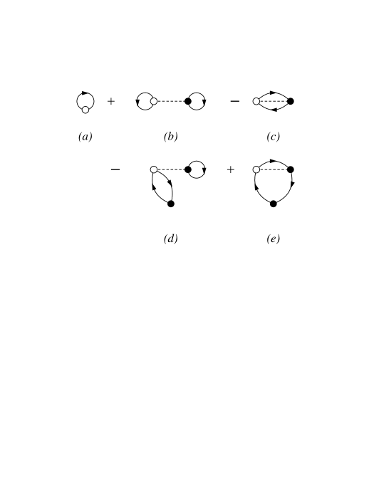
FIG. 1.: Diagrams representing the terms considered in our model for the calculation of the density distribution.

FIG. 2.: Correlation functions obtained for ¹²C and ⁴⁸Ca using the semi-realistic S3 nucleon–nucleon interaction. Dashed lines are gaussian correlations and full lines are the Euler correlation functions.

FIG. 3.: Comparison between densities (upper panels) and momentum distributions (lower panels) calculated with our model (dashed lines) and with a FHNC procedure (full lines). In all the panels the upper curves show the calculations done with Euler correlations, and the lower curves those done with gaussian correlations.

III The model: excited states

The description of nuclear responses in the quasi–elastic region is based upon the approach developed by Fantoni and Pandharipande [9] and applied to nuclear matter. The basic ansatz consists in assuming that the nuclear excited states can be described as a product of a Slater determinant and a many–body correlation function which is the same correlation function describing the ground state:

$$|\Psi_{f}\rangle=F|\Phi_{f}\rangle\,\,\,.$$ (10)

In eq. (10), $|\Phi_{f}\rangle$ indicates a Slater determinant which differs from $|\Phi_{0}\rangle$ by the fact that a certain number of hole single particle states have been substituted with particle wave functions.

The many–body nuclear response at energy $\omega$ and momentum transfer ${\bf q}$ to a an external field $Q({\bf q})$ can be written as:

$$R(\omega,{\bf q})=\sum_{f}\frac{\langle\Psi_{0}|Q^{+}({\bf q})|\Psi_{f}\rangle\langle\Psi_{f}|Q({\bf q})|\Psi_{0}\rangle}{\langle\Psi_{f}|\Psi_{f}\rangle\langle\Psi_{0}|\Psi_{0}\rangle}\,\,\,\delta(E_{f}-E_{0}-\omega)$$ (11)

where the sum is understood to run on all the nuclear excited states. The evaluation of eq. (11) requires the calculation of the full cluster expansion [9].

Like in the case of the density distribution, instead of performing the full expansion, after the elimination of the unlinked diagrams, we consider only the terms containing a single correlation function $h(r_{ij})$.

In the case the nuclear final state is characterized by one particle above the Fermi surface, the matrix element to be calculated are of the kind:

$$\xi_{ph}({\bf q})=\frac{\langle\Phi_{ph}|F^{+}Q^{+}({\bf q})F|\Phi_{0}\rangle}{\langle\Phi_{ph}|F^{+}F|\Phi_{0}\rangle}\,\,,$$ (12)

where we have indicated with $|\Phi_{ph}\rangle$ the Slater determinant where the hole single particle wave function $h$ has been substituted by the particle wave function $p$.

If the $Q$ operator is the charge operator, eq. (12) represents, in the limit for $q\rightarrow 0$ and $p\rightarrow h$, the normalization condition of the density. This fact allows us to identify the diagrams which we should consider to have a properly normalized many–body wave function. The diagrams we consider are shown in fig. 4. One can reconstruct the diagrams of fig. 1 by closing the particle and hole lines.

FIG. 4.: Diagrams considered in the calculation of the one-particle one-hole response. The symbols have the same meaning of those in fig 1. The black squares represent the point where the external field is acting on.

FIG. 5.: In $(a)$ the nuclear matter proton responses calculated with our model (dashed lines) are compared with those obtained with a full FHNC calculation (full lines). The lower panel show the difference between the responses calculated in the two approaches.

We have compared the nuclear matter charge responses calculated with our model [10] with those obtained with the FHNC procedure. The two calculations have been done with the gaussian correlation function of ¹²C of fig. 2. The comparison between the results of the two calculations is shown in fig. 5, where the dashed lines (our model) are almost exactly overlapped to the full ones (FHNC).

The excellent agreement between the two calculations has been obtained because we have included in our model, in order to have a correctly normalized many-body wave function, both two and three body terms. The effect of the three point diagrams can be seen in the figs. 6 and 7 where longitudinal an transverse responses for infinite nuclear matter and for the ¹²C nucleus are compared. We have used also for these calculations the ¹²C gaussian correlation of fig. 2. The finite system responses have been evaluated with the single particle wave functions producing the density shown in fig. 3.

In fig. 6, the left panels show the nuclear matter longitudinal responses for three different values of the momentum transfer. The full lines are the uncorrelated responses, i.e. the Fermi gas responses. The dotted lines have been obtained by evaluating only the two-points diagrams, while the results of the calculations where both two and three points diagrams have been taken into account are shown by the dashed lines. The effect of the inclusion of the three point diagrams has opposite sign with respect to that of the two points diagrams. This fact is not surprising since, in the normalization of the charge, the contribution of the the three points diagrams cancels exactly that of the two points diagrams. The finite size effect do not modify this conclusion as one can observe in the three right panels of the figure.

The calculation of the transverse response has been done by considering only the one-body magnetization current. The left panels of fig. 7 show the nuclear matter responses. Also in this case the effect of the three–points diagrams has opposite sign with respect to that of the two-points diagrams. We observe that the final response is extremely close to the uncorrelated response. The different behavior with respect to the case of the longitudinal response is produced by the fact that, for the nuclear matter transverse response, the diagrams $(d)$ and $(l)$ of fig. 4 do not contribute. This is strictly true only for the infinite system. In finite systems, only the diagram $d$ is zero. The right panels of fig. 7 show that this is the main responsible for the different behavior of the correlations in the longitudinal and the transverse response.

The model has been extended also to the case when the final state has two particles in the continuum [12], by using the same procedure described above for the 1p-1h excitation. In fig. 8 we show the longitudinal 2p-2h responses for three different values of the momentum transfer . The dashed lines have been obtained considering only the two points diagrams, while the full lines show the results obtained considering both two and three points diagrams. Also in this case the contribution of the three-points diagrams is relevant, close to the 40% for some value of the excitation energy.

It is necessary to remark that the absolute value of the response is three order of magnitude smaller than the 1p-1h response.

FIG. 6.: Longitudinal responses at various values of the momentum transfer calculated for 1p-1h excitation. The full lines represent the uncorrelated response the dotted lines the responses obtained by adding the two-points diagrams, and the dashed lined those obtained including also the three–points diagrams. The curves shown in the three left panels have been obtained for an infinite system while those shown in the right panels have been obtained for ¹²C using the wave functions giving the densities of fig. 3.

Figure 7. Same as in fig. 6 for the transverse responses.

IV Summary and conclusions

We have developed a model to describe nuclear responses taking into account short–range correlations. We have shown that mean values of the density operator can be calculated with minimal error by using a cluster expansion truncated up to the first order terms in the function $h(r_{ij})$. This truncation should be properly done to maintain the correct normalization of the wave function. This implies that both two and three points diagrams should be considered. We have shown that in both 1p-1h and 2p-2h responses the quantitative contribution of the three-point diagrams is relevant and cannot be simulated by multiplying the responses by a constant renormalization factor.

The calculations we have presented are limited to inclusive responses, but we plan to apply the model to treat exclusive processes.

Acknowledgments
This work has been partially supported by the agreement CICYT-INFN. S.R. would like to thank the Italian Foreigner Ministery for the financial support.

FIG. 8.: Charge response for 2p-2h excitation. The dashed lines represent the contribution of the two-points diagrams only, while the full lines show the result of the full calculation

REFERENCES

- [1] G. Co’, A. Fabrocini, S. Fantoni and I. Lagaris, Nucl. Phys. A 549, 439 (1992)
- [2] G. Co’, A. Fabrocini and S. Fantoni, Nucl. Phys. A 568, 73 (1994)
- [3] F. Arias de Saavedra, G. Co’, A. Fabrocini and S. Fantoni, Nucl. Phys. A 605, 359 (1996)
- [4] A. Fabrocini,F. Arias de Saavedra, G. Co’ and P. Folgarait, Phys. Rev. C 57, 1668 (1998)
- [5] contribution to this conference by F. Arias de Saavedra.
- [6] G. Co’, Nuovo Cimento 108A, 623 (1995)
- [7] F. Arias de Saavedra, G. Co’, and M.M. Renis, Phys. Rev. C 55, 673 (1997)
- [8] I.R.Afnan and Y.C.Tang, Phys. Rev. 17513371968
- [9] S. Fantoni and V.R. Pandharipande Nucl. Phys. A 473, 234 (1987)
- [10] J.E.Amaro, A.M. Lallena, G. Co’, and A. Fabrocini, Phys. Rev. C 57, 3473 (1998)
- [11] A. Fabrocini, Phys. Rev. C 55, 338 (1997)
- [12] G. Co’ and A.M.Lallena, Phys. Rev. C 57, 145 (1998)