Restoration of rotational invariance of bound states on the light front

Abstract

We study bound states in a model with scalar nucleons interacting via an exchanged scalar meson using the Hamiltonian formalism on the light front. In this approach manifest rotational invariance is broken when the Fock space is truncated. By considering an effective Hamiltonian that takes into account two meson exchanges, we find that this breaking of rotational invariance is decreased from that which occurs when only one meson exchange is included. The best improvement occurs when the states are weakly bound.

I Introduction

Covariant field theory can be coerced into giving solutions to non-perturbative problems such as bound states via the Bethe-Salpeter equation. There are technical difficulties in arriving at those solutions, but they are manifestly covariant. An alternative approach that also provides covariant results is obtained by using a Hamiltonian theory and the corresponding Schrödinger equation to solve for the bound states. A consequence of this covariance is that the commutation relations between the operators that constitute the four-momentum ($P^{\mu}$) and the four-angular momentum ($M^{\mu\nu}$) give a representation of the Poincaré algebra. There are many different formulations of Hamiltonian theories, corresponding to different forms of dynamics, as discussed by Dirac [1]. The components of the $P^{\mu}$ and $M^{\mu\nu}$ operators can be classified as either dynamic (dependent on the interaction) or kinematic. Different forms of dynamics result in different separations of $P^{\mu}$ and $M^{\mu\nu}$ into dynamic operators and kinematic operators. The two forms that we will be concerned with are the equal-time and light-front formalisms. The equal-time form gives four dynamical operators, while the light-front form yields only three dynamical ones. Having a small number of dynamical operators is good since this simplifies some calculations.

Using the canonical coordinate system, with $x^{\mu}=(x^{0},x^{1},x^{2},x^{3})$ and defining the commutation relations at equal time ($x^{0}=t$), we obtain the most familiar Hamiltonian theory, an equal-time theory. For this system, rotations and translations are kinematical, while the Hamiltonian and generators of boosts are dynamical. The fact that the generators of boosts are dynamical implies that when the full Hamiltonian is truncated, it will no longer transform appropriately under boosts. This implies that the equal-time Hamiltonian may not be well-suited for relativistic problems.

An alternative coordinate system is obtained by using light-front variables $x^{\pm}=x^{0}\pm x^{3}$ to construct $x^{\mu}=(x^{+},x^{-},x^{1},x^{2})$. High-energy experiments are naturally described using these coordinates, rather than equal-time ones. This is because the front of a beam traveling at the speed of light in the (negative) three-direction is defined by a surface where $x^{+}$ is constant. The description of the interaction of this beam with a target is much simpler if described in terms of light-front variables [2, 3] than if an equal-time variables are used. As an example, the Bjorken $x$ variable used to describe deep inelastic scattering experiments is simply the ratio of the plus momentum of the struck constituent particle to the total plus momentum of the bound state.

Using the light-front coordinate system and defining the commutation relations at equal light-front time ($x^{+}=t_{\text{LF}}$), we obtain a light-front Hamiltonian theory [2, 4, 5]. For this choice, rotation about the three axis, translations in the one, two, and plus directions, and the generators of boosts in the one, two, and plus directions are kinematical, while the Hamiltonian $(P^{-})$ and rotations about the one and two directions are dynamical. Since the boosts are kinematical, the light-front Hamiltonian is useful for relativistic problems, such as strongly-bound systems, even when the Hamiltonian is truncated. However, since two of the rotations are dynamical, the momentum operator four-vector will not be covariant under those rotations when the Hamiltonian is truncated. This lack of manifest rotational invariance presents some difficulties for bound-state calculations.

A key benefit of using the light front is that the vacuum can be very simple. For our theory, the masses of the particles are large. All massive particles and anti-particles have positive plus momentum, and the total plus momentum is a conserved quantity. Thus, there is no condensation, and the vacuum (with $p^{+}=0$) is empty, the Fock space vacuum. Thus, the Hilbert space for this theory is the Fock space. Diagrams that couple to the vacuum vanish, so the number of non-trivial light-front time-ordered diagrams is greatly reduced compared to the equal-time theory.

A Difficulties with the light front

An untruncated light-front Hamiltonian will commute with the total relative angular momentum operator, since the total momentum commutes with the relative momentum. Thus, for the scalar theory we consider here, the eigenstates of the full Hamiltonian will also be eigenstates of the angular momentum. However, as mentioned earlier, a Fock-space truncation of the light-front Hamiltonian results in the momentum operator four-vector losing covariance under rotations. Hence $J^{2}$ and the truncated Hamiltonian do not commute and this implies that the eigenstates of the truncated Hamiltonian will not be eigenstates of the angular momentum.

How will this violation of rotational invariance affect physical observables? A way to observe this violation is to note that on the light front, rotational invariance about the three-axis is maintained. This allows us to classify states as eigenstates of $J_{3}$ with eigenvalues $m$. We compare the energies of states with the same “relative angular momentum” quantum number $l$ but different $m$ values. We will define the “relative angular momentum” operator in section II C. If the Hamiltonian were rotationally invariant, the energies should be the same; the breaking of rotational invariance causes the energies to be different [6].

We expect that the higher Fock-space components of the full Hamiltonian will be small if the coupling constant is small enough. Thus, truncation at successively higher orders should reduce the violation of rotational invariance of the truncated Hamiltonian. In particular, by retaining enough terms in the perturbation expansion of the Hamiltonian, the violation of rotational invariance can be reduced to an arbitrarily small amount, provided only that a perturbation expansion is valid. Thus, the only real question is: How many terms are required?

B Outline of the rest of the paper

The purpose of this paper is to explore how truncation at different orders in the effective potential affects the breaking of rotational invariance of the spectra. The model we are using is a Lagrangian with neutral scalar particles coupled via a $\phi^{2}\chi$ interaction to other neutral scalar particles. The Bethe-Salpeter equation for this Lagrangian is discussed, and the ladder approximation to the Bethe-Salpeter equation and its spectra are reviewed. We also derive the light-front Hamiltonian from that Lagrangian and write out the light-front Schrödinger equation for bound states consisting of two particles. An approximation to the light-front potential that causes the light-front Schrödinger equation to be equivalent to the ladder Bethe-Salpeter equation is discussed. This approximation will be called the uncrossed approximation. The one-boson-exchange (OBE) effective potential and two-boson-exchange (TBE) effective potential are derived in this approximation. All of this is discussed in more detail in section II.

Following the development of the model, we look at some numerical calculations in section III. For our tests, we look at states composed of two massive scalar particles bound by the effects of the exchange of a lighter scalar particle. We calculate the spectra (the coupling constant versus bound-state mass curves) using the Bethe-Salpeter equation in the ladder approximation. Since the Bethe-Salpeter equation is manifestly covariant, its solutions are states with definite angular momentum. We also calculate the spectra using a light-front Schrödinger equation with the OBE and the OBE+TBE potentials. Because of the lack of manifest rotational invariance, these wavefunctions do not have definite angular momentum. An artificial “relative angular momentum” operator is constructed, and a partial-wave decomposition is performed on these wavefunctions to analyze the various angular momentum states present in them. The problem of trying to classify these states is discussed. We then plot the spectra for the wavefunctions classified as the lowest-lying $p$- and $d$-wave states for the Bethe-Salpeter, OBE Schrödinger, and the OBE+TBE Schrödinger equations.

In section IV, we summarize our findings: the higher-order terms help to partially restore the breaking of rotational invariance introduced by using only the OBE potential. This restoration is largest when the states are weakly bound.

We stress that the point of this paper is not to solve the Lagrangian of this model exactly. Instead, we seek to understand how rotational invariance is broken by the light-front Hamiltonian in the uncrossed approximation, how it can be partially restored by keeping higher-order graphs, and also to compare the results from the two truncated Hamiltonians to the results of the “exact” theory (the ladder Bethe-Salpeter equation). Discussion of the inclusion of the crossed-graph contributions will be given in a forthcoming paper [7].

This study is closely connected to the work of Schoonderwoerd, Bakker, and Karmanov [8], who considered two-body scattering in perturbation theory using a model similar to ours. Off-shell scattering amplitudes were computed at order $g^{4}$ and it was found that for low momenta, the TBE diagrams contributed much less than the iterated OBE diagrams. This lead to a conjecture that the lightly-bound states should be well described by the OBE potential, with the TBE potential playing a minor role. These results encourage us to calculate and compare bound states incorporating the OBE and OBE+TBE diagrams. We note that some of the difficulties present in [8] are avoided here since there are no singularities in the bound-state integral equation.

While this manuscript was in preparation, a paper by Sales et. al. [9] appeared. In that work, a model similar to ours was used to consider bound states. Their study included the same two truncations that we use, as well as the a comparison to the Bethe-Salpeter equation results. However, the investigation of Ref. [9] focused on the ground state, while here we are concerned with the rotational invariance of the excited states.

II Our model

We consider two distinguishable uncharged scalars $\phi=(\phi_{1},\phi_{2})$ with mass $M$ (which we will refer to as nucleons), that couple to a third, uncharged scalar $\chi$ with mass $\mu$ (which we will refer to as a meson) by a $\phi^{2}\chi$ interaction. This $\phi^{2}\chi$ theory, which can be considered a massive extension of the Wick-Cutkosky model [10], has been used by Schoonderwoerd, Bakker, and Karmanov [8] on the light front to study scattering states. The Lagrangian is

$$\mathcal{L} = \frac{1}{2}\left(\partial_{\mu}\phi\partial^{\mu}\phi-M^{2}\phi^{2}\right)+\frac{1}{2}\left(\partial_{\mu}\chi\partial^{\mu}\chi-\mu^{2}\chi^{2}\right)+\frac{gM}{2}\chi\phi^{2}.$$ (1)

This Lagrangian will be used in two formalisms, the Bethe-Salpeter equation and the Hamiltonian approach.

A Bethe-Salpeter equation

The Bethe-Salpeter equation [11, 12, 13, 14, 15] provides a way of describing bound states based on Feynman propagators and kernels constructed from covariant quantum field theory, and thus is manifestly covariant. The equation for the bound state of nucleons 1 and 2 can be written as

$$GK\psi = \psi,$$ (2)

$G$ is the free two-particle propagator, which is the product of two one-particle propagators, $G=S_{1}S_{2}$, $\psi$ is the four-dimensional Bethe-Salpeter amplitude, and $K$ is the sum of all two-particle irreducible two-to-two Feynman graphs,

$$K = \makebox[30.0pt]{\parbox{30.0pt}{\makebox[30.0pt]{ \immediate\ignorespaces\immediate\ignorespaces\immediate\ignorespaces\immediate\ignorespaces\immediate\ignorespaces{\f@ynmf:fmfriy\char 1\relax}\ignorespaces\immediate\ignorespaces\immediate\ignorespaces\immediate\ignorespaces\immediate\ignorespaces\immediate\ignorespaces\immediate\ignorespaces\immediate\ignorespaces\immediate\ignorespaces\immediate\ignorespaces\immediate\ignorespaces\immediate\ignorespaces\immediate\ignorespaces\immediate\ignorespaces\immediate\ignorespaces\immediate\ignorespaces\immediate\ignorespaces\immediate\ignorespaces\immediate\ignorespaces\immediate\ignorespaces\immediate\ignorespaces\immediate\ignorespaces \immediate\ignorespaces}}}+\makebox[30.0pt]{\parbox{30.0pt}{\makebox[30.0pt]{ \immediate\ignorespaces\immediate\ignorespaces\immediate\ignorespaces\immediate\ignorespaces\immediate\ignorespaces{\f@ynmf:fmfriy\char 2\relax}\ignorespaces\immediate\ignorespaces\immediate\ignorespaces\immediate\ignorespaces\immediate\ignorespaces\immediate\ignorespaces\immediate\ignorespaces\immediate\ignorespaces\immediate\ignorespaces\immediate\ignorespaces\immediate\ignorespaces\immediate\ignorespaces\immediate\ignorespaces\immediate\ignorespaces\immediate\ignorespaces\immediate\ignorespaces\immediate\ignorespaces\immediate\ignorespaces\immediate\ignorespaces\immediate\ignorespaces\immediate\ignorespaces\immediate\ignorespaces\immediate\ignorespaces\immediate\ignorespaces\immediate\ignorespaces \immediate\ignorespaces}}}+\makebox[30.0pt]{\parbox{30.0pt}{\makebox[30.0pt]{ \immediate\ignorespaces\immediate\ignorespaces\immediate\ignorespaces\immediate\ignorespaces\immediate\ignorespaces{\f@ynmf:fmfriy\char 3\relax}\ignorespaces\immediate\ignorespaces\immediate\ignorespaces\immediate\ignorespaces\immediate\ignorespaces\immediate\ignorespaces\immediate\ignorespaces\immediate\ignorespaces\immediate\ignorespaces\immediate\ignorespaces\immediate\ignorespaces\immediate\ignorespaces\immediate\ignorespaces\immediate\ignorespaces\immediate\ignorespaces\immediate\ignorespaces\immediate\ignorespaces\immediate\ignorespaces\immediate\ignorespaces\immediate\ignorespaces\immediate\ignorespaces\immediate\ignorespaces\immediate\ignorespaces\immediate\ignorespaces\immediate\ignorespaces \immediate\ignorespaces}}}+\makebox[30.0pt]{\parbox{30.0pt}{\makebox[30.0pt]{ \immediate\ignorespaces\immediate\ignorespaces\immediate\ignorespaces\immediate\ignorespaces\immediate\ignorespaces{\f@ynmf:fmfriy\char 4\relax}\ignorespaces\immediate\ignorespaces\immediate\ignorespaces\immediate\ignorespaces\immediate\ignorespaces\immediate\ignorespaces\immediate\ignorespaces\immediate\ignorespaces\immediate\ignorespaces\immediate\ignorespaces\immediate\ignorespaces\immediate\ignorespaces\immediate\ignorespaces\immediate\ignorespaces\immediate\ignorespaces\immediate\ignorespaces\immediate\ignorespaces\immediate\ignorespaces\immediate\ignorespaces\immediate\ignorespaces\immediate\ignorespaces\immediate\ignorespaces\immediate\ignorespaces\immediate\ignorespaces\immediate\ignorespaces \immediate\ignorespaces}}}+\makebox[30.0pt]{\parbox{30.0pt}{\makebox[30.0pt]{ \immediate\ignorespaces\immediate\ignorespaces\immediate\ignorespaces\immediate\ignorespaces\immediate\ignorespaces{\f@ynmf:fmfriy\char 5\relax}\ignorespaces\immediate\ignorespaces\immediate\ignorespaces\immediate\ignorespaces\immediate\ignorespaces\immediate\ignorespaces\immediate\ignorespaces\immediate\ignorespaces\immediate\ignorespaces\immediate\ignorespaces\immediate\ignorespaces\immediate\ignorespaces\immediate\ignorespaces\immediate\ignorespaces\immediate\ignorespaces\immediate\ignorespaces\immediate\ignorespaces\immediate\ignorespaces\immediate\ignorespaces\immediate\ignorespaces\immediate\ignorespaces\immediate\ignorespaces\immediate\ignorespaces\immediate\ignorespaces\immediate\ignorespaces\immediate\ignorespaces\immediate\ignorespaces\immediate\ignorespaces\immediate\ignorespaces\immediate\ignorespaces\immediate\ignorespaces \immediate\ignorespaces}}}+\cdots\,.$$ (3)

There are no nucleon exchange graphs since we treat only the case where the two nucleons are distinguishable.

We consider the ladder approximation to the Bethe-Salpeter equation,

$$g^{2}GK_{\text{OBE}}\psi = \psi,$$ (4)

which is obtained by replacing $K$ in Eq. (2) with $g^{2}K_{\text{OBE}}$, the graph due to one-boson-exchange,

$$K_{\text{OBE}} = \frac{1}{g^{2}}\makebox[30.0pt]{\parbox{30.0pt}{\makebox[30.0pt]{ \immediate\ignorespaces\immediate\ignorespaces\immediate\ignorespaces\immediate\ignorespaces\immediate\ignorespaces{\f@ynmf:fmfriy\char 6\relax}\ignorespaces\immediate\ignorespaces\immediate\ignorespaces\immediate\ignorespaces\immediate\ignorespaces\immediate\ignorespaces\immediate\ignorespaces\immediate\ignorespaces\immediate\ignorespaces\immediate\ignorespaces\immediate\ignorespaces\immediate\ignorespaces\immediate\ignorespaces\immediate\ignorespaces\immediate\ignorespaces\immediate\ignorespaces\immediate\ignorespaces\immediate\ignorespaces\immediate\ignorespaces\immediate\ignorespaces\immediate\ignorespaces\immediate\ignorespaces \immediate\ignorespaces}}}.$$ (5)

This definition of $K_{\text{OBE}}$ makes it independent of the coupling constant. Making this approximation leaves the Bethe-Salpeter equation covariant. This implies that the Bethe-Salpeter amplitudes $\psi$ have definite angular momentum $l$, and hence the energies of the states are degenerate for different $m$ projections of the same angular momentum.

This equation can be simplified in the center-of-momentum frame. In that frame, once the total energy is defined as $P^{0}$, the four-momentum of the second particle is given by $k_{2}^{\mu}=P^{\mu}-k_{1}^{\mu}$, and thus the Bethe-Salpeter equation is effectively a one-particle equation. The remainder of the discussion in this section will be done in the c.m. frame. We then can rewrite Eq. (4), taking into account the explicit symmetries of the equation, as

$$\left[g_{\text{LBSE}}^{n,l,m}(E)\right]^{2}G(E)K_{\text{OBE}}(E)\psi_{n,l,m} = \psi_{n,l,m},$$ (6)

where $E$ is an arbitrary energy, $\psi_{n,l,m}$ is the $n^{\text{th}}$ Bethe-Salpeter amplitude with angular momentum $l$ and three-projection $m$, and $g_{\text{LBSE}}^{n,l,m}(E)$ is the coupling constant which yields that bound-state Bethe-Salpeter amplitude with $E$ as the bound-state energy. We call this $g(E)$ the spectrum of the ladder Bethe-Salpeter equation for the corresponding Bethe-Salpeter amplitude. The Greens function $G(E)$ and the OBE kernel $K_{\text{OBE}}(E)$ are functions of the energy in the c.m. frame and are implicitly effective one-particle operators.

The comparison we draw is only between the ladder Bethe-Salpeter equation and the light-front Hamiltonian that corresponds to that approximation. The exact nature of the correspondence is discussed in section II C. Since we are not looking at the solutions to the full theory, for our purposes it does not matter that there are sizeable differences between the solutions to the full Bethe-Salpeter equation and the ladder approximation when the coupling constant is large [16, 17, 18, 19].

B Light-front Hamiltonian

To obtain the light-front Hamiltonian from the Lagrangian in Eq. (1), we follow the approach used by Miller [3] and many others (see the review [2]) to write the light-front Hamiltonian ($P^{-}$) as the sum of a free, non-interacting part and a term containing the interactions. This is accomplished by using the energy-momentum tensor in

$$P^{\mu}={1\over 2}\int dx^{-}d^{2}x_{\perp}\;T^{+\mu}(x^{+}=0,x^{-},\mathchoice{{\hbox{\boldmath$\displaystyle x$}}}{{\hbox{\boldmath$\textstyle x$}}}{{\hbox{\boldmath$\scriptstyle x$}}}{{\hbox{\boldmath$\scriptscriptstyle x$}}}_{\perp}).$$ (7)

The usual relations determine $T^{+\mu}$, with

$$T^{\mu\nu}=-g^{\mu\nu}{\cal L}+\sum_{r}{\partial{\cal L}\over\partial(\partial_{\mu}\phi_{r})}\partial^{\nu}\phi_{r},$$ (8)

in which the degrees of freedom are labeled by $\phi_{r}$.

It is worthwhile to consider the limit in which the interactions between the fields are removed. This will allow us to define the free Hamiltonian $P^{-}_{0}$ and to display the necessary commutation relations. The energy-momentum tensor of the non-interacting fields is defined as $T_{0}^{\mu\nu}$. Use of Eq. (8) leads to the result

$$T^{\mu\nu}_{0} = \partial^{\mu}\phi\partial^{\nu}\phi-\frac{g^{\mu\nu}}{2}\left[\partial_{\sigma}\phi\partial^{\sigma}\phi-M^{2}\phi^{2}\right]+\partial^{\mu}\chi\partial^{\nu}\chi-\frac{g^{\mu\nu}}{2}\left[\partial_{\sigma}\chi\partial^{\sigma}\chi-\mu^{2}\chi^{2}\right],$$ (9)

with

$$T^{+-}_{0}=\mathchoice{{\hbox{\boldmath$\displaystyle\nabla$}}}{{\hbox{\boldmath$\textstyle\nabla$}}}{{\hbox{\boldmath$\scriptstyle\nabla$}}}{{\hbox{\boldmath$\scriptscriptstyle\nabla$}}}_{\perp}\phi\cdot\mathchoice{{\hbox{\boldmath$\displaystyle\nabla$}}}{{\hbox{\boldmath$\textstyle\nabla$}}}{{\hbox{\boldmath$\scriptstyle\nabla$}}}{{\hbox{\boldmath$\scriptscriptstyle\nabla$}}}_{\perp}\phi+M^{2}\phi^{2}+\mathchoice{{\hbox{\boldmath$\displaystyle\nabla$}}}{{\hbox{\boldmath$\textstyle\nabla$}}}{{\hbox{\boldmath$\scriptstyle\nabla$}}}{{\hbox{\boldmath$\scriptscriptstyle\nabla$}}}_{\perp}\chi\cdot\mathchoice{{\hbox{\boldmath$\displaystyle\nabla$}}}{{\hbox{\boldmath$\textstyle\nabla$}}}{{\hbox{\boldmath$\scriptstyle\nabla$}}}{{\hbox{\boldmath$\scriptscriptstyle\nabla$}}}_{\perp}\chi+\mu^{2}\chi^{2}.$$ (10)

The scalar nucleon fields can be expressed in terms of creation and destruction operators:

$$\phi_{i}(x) = \int\frac{d^{2}k_{\perp}dk^{+}\,\theta(k^{+})}{(2\pi)^{3/2}\sqrt{2k^{+}}}\left[a_{i}(\mathchoice{{\hbox{\boldmath$\displaystyle k$}}}{{\hbox{\boldmath$\textstyle k$}}}{{\hbox{\boldmath$\scriptstyle k$}}}{{\hbox{\boldmath$\scriptscriptstyle k$}}})e^{-ik\cdot x}+a_{i}^{\dagger}(\mathchoice{{\hbox{\boldmath$\displaystyle k$}}}{{\hbox{\boldmath$\textstyle k$}}}{{\hbox{\boldmath$\scriptstyle k$}}}{{\hbox{\boldmath$\scriptscriptstyle k$}}})e^{ik\cdot x}\right],$$ (11)

where $i=1,2$ is a particle index, $k\cdot x={1\over 2}(k^{-}x^{+}+k^{+}x^{-})-\mathchoice{{\hbox{\boldmath$\displaystyle k$}}}{{\hbox{\boldmath$\textstyle k$}}}{{\hbox{\boldmath$\scriptstyle k$}}}{{\hbox{\boldmath$\scriptscriptstyle k$}}}_{\perp}\cdot\mathchoice{{\hbox{\boldmath$\displaystyle x$}}}{{\hbox{\boldmath$\textstyle x$}}}{{\hbox{\boldmath$\scriptstyle x$}}}{{\hbox{\boldmath$\scriptscriptstyle x$}}}_{\perp}$ with $k^{-}=\frac{M^{2}+\mathchoice{{\hbox{\boldmath$\displaystyle k$}}}{{\hbox{\boldmath$\textstyle k$}}}{{\hbox{\boldmath$\scriptstyle k$}}}{{\hbox{\boldmath$\scriptscriptstyle k$}}}_{\perp}^{2}}{k^{+}}$, and $\mathchoice{{\hbox{\boldmath$\displaystyle k$}}}{{\hbox{\boldmath$\textstyle k$}}}{{\hbox{\boldmath$\scriptstyle k$}}}{{\hbox{\boldmath$\scriptscriptstyle k$}}}\equiv(k^{+},\mathchoice{{\hbox{\boldmath$\displaystyle k$}}}{{\hbox{\boldmath$\textstyle k$}}}{{\hbox{\boldmath$\scriptstyle k$}}}{{\hbox{\boldmath$\scriptscriptstyle k$}}}_{\perp})$. Note that $k^{-}$ is such that the particles are on the mass shell, which is a consequence of using a Hamiltonian theory. The $\theta$ function restricts $k^{+}$ to positive values. Likewise, the scalar meson field is given by

$$\chi(x) = \int\frac{d^{2}k_{\perp}dk^{+}\,\theta(k^{+})}{(2\pi)^{3/2}\sqrt{2k^{+}}}\left[a_{\chi}(\mathchoice{{\hbox{\boldmath$\displaystyle k$}}}{{\hbox{\boldmath$\textstyle k$}}}{{\hbox{\boldmath$\scriptstyle k$}}}{{\hbox{\boldmath$\scriptscriptstyle k$}}})e^{-ik\cdot x}+a_{\chi}^{\dagger}(\mathchoice{{\hbox{\boldmath$\displaystyle k$}}}{{\hbox{\boldmath$\textstyle k$}}}{{\hbox{\boldmath$\scriptstyle k$}}}{{\hbox{\boldmath$\scriptscriptstyle k$}}})e^{ik\cdot x}\right],$$ (12)

where $k^{-}=\frac{\mu^{2}+\mathchoice{{\hbox{\boldmath$\displaystyle k$}}}{{\hbox{\boldmath$\textstyle k$}}}{{\hbox{\boldmath$\scriptstyle k$}}}{{\hbox{\boldmath$\scriptscriptstyle k$}}}_{\perp}^{2}}{k^{+}}$, so that the mesons are also on the mass shell. The non-vanishing commutation relations are

$$\left[a_{\alpha}(\mathchoice{{\hbox{\boldmath$\displaystyle k$}}}{{\hbox{\boldmath$\textstyle k$}}}{{\hbox{\boldmath$\scriptstyle k$}}}{{\hbox{\boldmath$\scriptscriptstyle k$}}}),a_{\alpha}^{\dagger}(\mathchoice{{\hbox{\boldmath$\displaystyle k$}}}{{\hbox{\boldmath$\textstyle k$}}}{{\hbox{\boldmath$\scriptstyle k$}}}{{\hbox{\boldmath$\scriptscriptstyle k$}}}^{\prime})\right] = \delta(\mathchoice{{\hbox{\boldmath$\displaystyle k$}}}{{\hbox{\boldmath$\textstyle k$}}}{{\hbox{\boldmath$\scriptstyle k$}}}{{\hbox{\boldmath$\scriptscriptstyle k$}}}_{\perp}-\mathchoice{{\hbox{\boldmath$\displaystyle k$}}}{{\hbox{\boldmath$\textstyle k$}}}{{\hbox{\boldmath$\scriptstyle k$}}}{{\hbox{\boldmath$\scriptscriptstyle k$}}}^{\prime}_{\perp})\delta(k^{+}-k^{\prime+}),$$ (13)

where $\alpha=1,2,\chi$ is a particle index. The commutation relations are defined at equal light-front time, $x^{+}=0$.

The derivatives appearing in the quantity $T^{+-}_{0}$ are evaluated and then one sets $x^{+}$ to 0 to obtain the result

$$P^{-}_{0} = \int_{k}\,\left[\frac{M^{2}+\mathchoice{{\hbox{\boldmath$\displaystyle k$}}}{{\hbox{\boldmath$\textstyle k$}}}{{\hbox{\boldmath$\scriptstyle k$}}}{{\hbox{\boldmath$\scriptscriptstyle k$}}}_{\perp}^{2}}{k^{+}}\left(a_{1}^{\dagger}(k)a_{1}(k)+a_{2}^{\dagger}(k)a_{2}(k)\right)+\frac{\mu^{2}+\mathchoice{{\hbox{\boldmath$\displaystyle k$}}}{{\hbox{\boldmath$\textstyle k$}}}{{\hbox{\boldmath$\scriptstyle k$}}}{{\hbox{\boldmath$\scriptscriptstyle k$}}}_{\perp}^{2}}{k^{+}}a_{\chi}^{\dagger}(k)a_{\chi}(k)\right],$$ (14)

with $\int_{k}=\int d^{2}k_{\perp}dk^{+}\,\theta(k^{+})$. Eq. (14) has the interpretation of an operator that counts the light-front energy $k^{-}$ (which is $\frac{M^{2}+\mathchoice{{\hbox{\boldmath$\displaystyle k$}}}{{\hbox{\boldmath$\textstyle k$}}}{{\hbox{\boldmath$\scriptstyle k$}}}{{\hbox{\boldmath$\scriptscriptstyle k$}}}_{\perp}^{2}}{k^{+}}$ for the nucleons and $\frac{\mu^{2}+\mathchoice{{\hbox{\boldmath$\displaystyle k$}}}{{\hbox{\boldmath$\textstyle k$}}}{{\hbox{\boldmath$\scriptstyle k$}}}{{\hbox{\boldmath$\scriptscriptstyle k$}}}_{\perp}^{2}}{k^{+}}$ for the mesons) of all of the particles.

We now consider the interacting part of the Lagrangian, ${\mathcal{L}}_{I}$. An analysis similar to that for the non-interacting parts yields the interacting part of the light-front Hamiltonian $P_{I}^{-}$;

$$P_{I}^{-} = \sum_{i=1,2}\frac{gM}{2}\int_{k}\int_{k^{\prime}}\frac{1}{(2\pi)^{3/2}\sqrt{2k^{+}k^{\prime+}(k^{+}+k^{\prime+})}}$$ (17)

$$\phantom{\sum_{i=1,2}\frac{gM}{2}\int_{k}\int_{k^{\prime}}}\times\left\{\left[2a_{i}^{\dagger}(k+k^{\prime})a_{\chi}(k^{\prime})a_{i}(k)+a_{\chi}^{\dagger}(k+k^{\prime})a_{i}(k^{\prime})a_{i}(k)\right]\right.$$

$$\phantom{\sum_{i=1,2}\frac{gM}{2}\int_{k}\int_{k^{\prime}}\times\left\{\right.}\left.+\mbox{Hermitian conjugate}\right\}.$$

For our theory, the Hilbert space is the Fock space. Eq. (17) is self-adjoint on that Hilbert space, since the equation is written in terms of the Fock operators. The total light-front Hamiltonian is given by $P^{-}=P^{-}_{0}+P^{-}_{I}$.

C Hamiltonian bound-state equations

We will be studying the bound states of two distinguishable nucleons in the light-front analogue of old-fashioned (time-ordered) perturbation theory: light-front time-ordered perturbation theory (LFTOPT). Using this perturbation theory for our Hamiltonian, we can write out a two-nucleon effective Hamiltonian “eigenvalue” equation (a light-front Schrödinger equation) where the potential is expanded in powers of the coupling constant $g$. This is not a true eigenvalue equation since the potential is energy dependent. We write this in the form of Eq. (6)

$$\left[P_{0}^{-}+V\Big{(}g^{n}_{\text{LFSE}}(P^{-}),P^{-}\Big{)}\right]|\psi^{n}\rangle = |\psi^{n}\rangle P^{-}$$ (18)

$$V(g,P^{-}) = \sum_{i=1}^{\infty}g^{2i}V_{(2i)}(P^{-}),$$ (19)

where $P^{-}$ is an arbitrary light-front energy, $|\psi^{n}\rangle$ is the the $n^{\text{th}}$ wavefunction, and $g^{n}_{\text{LFSE}}(P^{-})$ is the coupling constant which yields that bound-state wavefunction with $P^{-}$ as the bound-state energy. We call this $g(P^{-})$ the spectrum of the light-front Schrödinger equation for the corresponding wavefunction. Only even powers of $g$ appear in $V$ since every meson emitted must be absorbed. Also, since $V_{(2i)}$ is the potential due to the exchange of $i$ mesons, we call $V_{(2)}=V_{\text{OBE}}$ and $V_{(4)}=V_{\text{TBE}}$. The potentials $V_{(2i)}$ can be calculated from the light-front time-ordered diagrams.

We want to approximate our potential $V$ so that Eq. (18) is physically equivalent to the ladder Bethe-Salpeter equation. This approximation of $V$ will be called the uncrossed approximation. By physically equivalent, we mean that the spectra of the potential $V$ should reproduce the spectrum for the states of the Bethe-Salpeter equation, excluding the so-called “abnormal” states [10]. It is well known how to reduce the Bethe-Salpeter equation to a physically equivalent Hamiltonian (Schrödinger-type) equation. For an extensive discussion of this issue of defining the potential equivalent to a sum of Feynman graphs in the equal-time case see, for instance, Klein [20], Phillips and Wallace [21], Lahiff and Afnan [22], and for examples on the light front, Ligterink and Bakker [23]. The general procedure to get the effective potential due to $n$ boson exchange takes two steps. First, write the sum of all Feynman graphs obtained from iteration of the Bethe-Salpeter kernel with $n$ boson exchanges. Then, write that sum in terms of LFTOPT graphs, and discard all graphs which are not two-particle-irreducible with respect to the light-front two-body propagator,

$$G_{\text{LF}}\left(P^{-}\right) = \frac{1}{P^{-}-P^{-}_{0}}.$$ (20)

The graphs which remain after this procedure constitute the $V_{\text{nBE}}$.

As an example, we construct the TBE potential. When the ladder Bethe-Salpeter equation is used, only one Feynman graph contributes, the box diagram arising from the iteration of the Feynman OBE kernel. This gives six non-vanishing LFTOPT diagrams. (The other diagrams vanish because the vacuum is simple on the light front.)

$$\left(\,\makebox[30.0pt]{\parbox{30.0pt}{\makebox[30.0pt]{ \immediate\ignorespaces\immediate\ignorespaces\immediate\ignorespaces\immediate\ignorespaces\immediate\ignorespaces{\f@ynmf:fmfriy\char 7\relax}\ignorespaces\immediate\ignorespaces\immediate\ignorespaces\immediate\ignorespaces\immediate\ignorespaces\immediate\ignorespaces\immediate\ignorespaces\immediate\ignorespaces\immediate\ignorespaces\immediate\ignorespaces\immediate\ignorespaces\immediate\ignorespaces\immediate\ignorespaces\immediate\ignorespaces\immediate\ignorespaces\immediate\ignorespaces\immediate\ignorespaces\immediate\ignorespaces\immediate\ignorespaces\immediate\ignorespaces\immediate\ignorespaces\immediate\ignorespaces\immediate\ignorespaces\immediate\ignorespaces\immediate\ignorespaces \immediate\ignorespaces}}}\,\right)_{\mbox{Feynman}} = \,\makebox[30.0pt]{\parbox{30.0pt}{\makebox[30.0pt]{ \immediate\ignorespaces\immediate\ignorespaces\immediate\ignorespaces\immediate\ignorespaces\immediate\ignorespaces{\f@ynmf:fmfriy\char 8\relax}\ignorespaces\immediate\ignorespaces\immediate\ignorespaces\immediate\ignorespaces\immediate\ignorespaces\immediate\ignorespaces\immediate\ignorespaces\immediate\ignorespaces\immediate\ignorespaces\immediate\ignorespaces\immediate\ignorespaces\immediate\ignorespaces\immediate\ignorespaces\immediate\ignorespaces\immediate\ignorespaces\immediate\ignorespaces\immediate\ignorespaces\immediate\ignorespaces\immediate\ignorespaces\immediate\ignorespaces\immediate\ignorespaces\immediate\ignorespaces\immediate\ignorespaces\immediate\ignorespaces\immediate\ignorespaces \immediate\ignorespaces}}}\,+\,\makebox[30.0pt]{\parbox{30.0pt}{\makebox[30.0pt]{ \immediate\ignorespaces\immediate\ignorespaces\immediate\ignorespaces\immediate\ignorespaces\immediate\ignorespaces{\f@ynmf:fmfriy\char 9\relax}\ignorespaces\immediate\ignorespaces\immediate\ignorespaces\immediate\ignorespaces\immediate\ignorespaces\immediate\ignorespaces\immediate\ignorespaces\immediate\ignorespaces\immediate\ignorespaces\immediate\ignorespaces\immediate\ignorespaces\immediate\ignorespaces\immediate\ignorespaces\immediate\ignorespaces\immediate\ignorespaces\immediate\ignorespaces\immediate\ignorespaces\immediate\ignorespaces\immediate\ignorespaces\immediate\ignorespaces\immediate\ignorespaces\immediate\ignorespaces\immediate\ignorespaces\immediate\ignorespaces\immediate\ignorespaces \immediate\ignorespaces}}}\,+\,\makebox[30.0pt]{\parbox{30.0pt}{\makebox[30.0pt]{ \immediate\ignorespaces\immediate\ignorespaces\immediate\ignorespaces\immediate\ignorespaces\immediate\ignorespaces{\f@ynmf:fmfriy\char 10\relax}\ignorespaces\immediate\ignorespaces\immediate\ignorespaces\immediate\ignorespaces\immediate\ignorespaces\immediate\ignorespaces\immediate\ignorespaces\immediate\ignorespaces\immediate\ignorespaces\immediate\ignorespaces\immediate\ignorespaces\immediate\ignorespaces\immediate\ignorespaces\immediate\ignorespaces\immediate\ignorespaces\immediate\ignorespaces\immediate\ignorespaces\immediate\ignorespaces\immediate\ignorespaces\immediate\ignorespaces\immediate\ignorespaces\immediate\ignorespaces\immediate\ignorespaces\immediate\ignorespaces\immediate\ignorespaces \immediate\ignorespaces}}}\,+\,\makebox[30.0pt]{\parbox{30.0pt}{\makebox[30.0pt]{ \immediate\ignorespaces\immediate\ignorespaces\immediate\ignorespaces\immediate\ignorespaces\immediate\ignorespaces{\f@ynmf:fmfriy\char 11\relax}\ignorespaces\immediate\ignorespaces\immediate\ignorespaces\immediate\ignorespaces\immediate\ignorespaces\immediate\ignorespaces\immediate\ignorespaces\immediate\ignorespaces\immediate\ignorespaces\immediate\ignorespaces\immediate\ignorespaces\immediate\ignorespaces\immediate\ignorespaces\immediate\ignorespaces\immediate\ignorespaces\immediate\ignorespaces\immediate\ignorespaces\immediate\ignorespaces\immediate\ignorespaces\immediate\ignorespaces\immediate\ignorespaces\immediate\ignorespaces\immediate\ignorespaces\immediate\ignorespaces\immediate\ignorespaces \immediate\ignorespaces}}}\,+\,\makebox[30.0pt]{\parbox{30.0pt}{\makebox[30.0pt]{ \immediate\ignorespaces\immediate\ignorespaces\immediate\ignorespaces\immediate\ignorespaces\immediate\ignorespaces{\f@ynmf:fmfriy\char 12\relax}\ignorespaces\immediate\ignorespaces\immediate\ignorespaces\immediate\ignorespaces\immediate\ignorespaces\immediate\ignorespaces\immediate\ignorespaces\immediate\ignorespaces\immediate\ignorespaces\immediate\ignorespaces\immediate\ignorespaces\immediate\ignorespaces\immediate\ignorespaces\immediate\ignorespaces\immediate\ignorespaces\immediate\ignorespaces\immediate\ignorespaces\immediate\ignorespaces\immediate\ignorespaces\immediate\ignorespaces\immediate\ignorespaces\immediate\ignorespaces\immediate\ignorespaces\immediate\ignorespaces\immediate\ignorespaces \immediate\ignorespaces}}}\,+\,\makebox[30.0pt]{\parbox{30.0pt}{\makebox[30.0pt]{ \immediate\ignorespaces\immediate\ignorespaces\immediate\ignorespaces\immediate\ignorespaces\immediate\ignorespaces{\f@ynmf:fmfriy\char 13\relax}\ignorespaces\immediate\ignorespaces\immediate\ignorespaces\immediate\ignorespaces\immediate\ignorespaces\immediate\ignorespaces\immediate\ignorespaces\immediate\ignorespaces\immediate\ignorespaces\immediate\ignorespaces\immediate\ignorespaces\immediate\ignorespaces\immediate\ignorespaces\immediate\ignorespaces\immediate\ignorespaces\immediate\ignorespaces\immediate\ignorespaces\immediate\ignorespaces\immediate\ignorespaces\immediate\ignorespaces\immediate\ignorespaces\immediate\ignorespaces\immediate\ignorespaces\immediate\ignorespaces\immediate\ignorespaces \immediate\ignorespaces}}}\,.$$ (21)

The first four diagrams are iterations of the OBE potential and are reducible with respect to $G_{\text{LF}}$. The last two are two-particle-irreducible and thus constitute the TBE potential, $V_{\text{TBE}}$.

A truncation must be made for the potential in Eq. (19), since in this Hamiltonian theory the infinite sum of graphs (required to reproduce the covariant results of the Bethe-Salpeter equation) cannot be calculated. In this paper we consider two truncations, one where we only keep the OBE potential, and another where we keep OBE and TBE potentials. We write out the matrix elements of $V_{\text{OBE}}$ and $V_{\text{TBE}}$ in the two-particle momentum basis, denoting the momentum of the incoming particles by $p_{1}$ and $p_{2}$, and the outgoing particles $k_{1}$ and $k_{2}$. For $V_{\text{TBE}}$, particles 1 and 2 have intermediate momenta which we denote by $q_{1}$ and $q_{2}$. In terms of diagrams, the potentials are

$$V_{\text{OBE}} = \qquad\makebox[45.0pt]{\parbox{45.0pt}{\makebox[45.0pt]{ \begin{picture}(45.0,30.0)\immediate\ignorespaces\immediate\ignorespaces\immediate\ignorespaces\immediate\ignorespaces\immediate\ignorespaces{\immediate\immediate}\put(0.0,0.0){{\f@ynmf:fmfriy\char 14\relax}}\ignorespaces\immediate\ignorespaces\immediate\ignorespaces\immediate\ignorespaces\immediate\ignorespaces\immediate\ignorespaces\immediate\ignorespaces\immediate\ignorespaces\immediate\ignorespaces\immediate\ignorespaces\immediate\ignorespaces\immediate\ignorespaces\immediate\ignorespaces\immediate\ignorespaces\immediate\ignorespaces\immediate\ignorespaces\immediate\ignorespaces\immediate\ignorespaces\immediate\ignorespaces\immediate\ignorespaces\immediate\ignorespaces\immediate\ignorespaces\immediate\ignorespaces\immediate\ignorespaces\immediate\ignorespaces\immediate\ignorespaces\immediate\ignorespaces \immediate\ignorespaces{\put(28.56178,14.99602){\makebox(0.0,0.0)[l]{$p_{1}-k_{1}$}} \put(-5.04866,-3.3658){\makebox(0.0,0.0)[rt]{$k_{2}$}} \put(-5.04866,33.35785){\makebox(0.0,0.0)[rb]{$k_{1}$}} \put(50.03673,-3.3658){\makebox(0.0,0.0)[lt]{$p_{2}$}} \put(50.03673,33.35785){\makebox(0.0,0.0)[lb]{$p_{1}$}} }\end{picture}}}}\qquad+\qquad\makebox[45.0pt]{\parbox{45.0pt}{\makebox[45.0pt]{ \begin{picture}(45.0,30.0)\immediate\ignorespaces\immediate\ignorespaces\immediate\ignorespaces\immediate\ignorespaces\immediate\ignorespaces{\immediate\immediate}\put(0.0,0.0){{\f@ynmf:fmfriy\char 15\relax}}\ignorespaces\immediate\ignorespaces\immediate\ignorespaces\immediate\ignorespaces\immediate\ignorespaces\immediate\ignorespaces\immediate\ignorespaces\immediate\ignorespaces\immediate\ignorespaces\immediate\ignorespaces\immediate\ignorespaces\immediate\ignorespaces\immediate\ignorespaces\immediate\ignorespaces\immediate\ignorespaces\immediate\ignorespaces\immediate\ignorespaces\immediate\ignorespaces\immediate\ignorespaces\immediate\ignorespaces\immediate\ignorespaces\immediate\ignorespaces\immediate\ignorespaces\immediate\ignorespaces\immediate\ignorespaces\immediate\ignorespaces\immediate\ignorespaces \immediate\ignorespaces{\put(28.56178,14.99602){\makebox(0.0,0.0)[l]{$k_{1}-p_{1}$}} \put(-5.04866,-3.3658){\makebox(0.0,0.0)[rt]{$k_{2}$}} \put(-5.04866,33.35785){\makebox(0.0,0.0)[rb]{$k_{1}$}} \put(50.03673,-3.3658){\makebox(0.0,0.0)[lt]{$p_{2}$}} \put(50.03673,33.35785){\makebox(0.0,0.0)[lb]{$p_{1}$}} }\end{picture}}}}$$ (23)

$$V_{\text{TBE}} = \qquad\makebox[45.0pt]{\parbox{45.0pt}{\makebox[45.0pt]{ \begin{picture}(45.0,30.0)\immediate\ignorespaces\immediate\ignorespaces\immediate\ignorespaces\immediate\ignorespaces\immediate\ignorespaces{\immediate\immediate}\put(0.0,0.0){{\f@ynmf:fmfriy\char 16\relax}}\ignorespaces\immediate\ignorespaces\immediate\ignorespaces\immediate\ignorespaces\immediate\ignorespaces\immediate\ignorespaces\immediate\ignorespaces\immediate\ignorespaces\immediate\ignorespaces\immediate\ignorespaces\immediate\ignorespaces\immediate\ignorespaces\immediate\ignorespaces\immediate\ignorespaces\immediate\ignorespaces\immediate\ignorespaces\immediate\ignorespaces\immediate\ignorespaces\immediate\ignorespaces\immediate\ignorespaces\immediate\ignorespaces\immediate\ignorespaces\immediate\ignorespaces\immediate\ignorespaces\immediate\ignorespaces\immediate\ignorespaces\immediate\ignorespaces\immediate\ignorespaces\immediate\ignorespaces\immediate\ignorespaces\immediate\ignorespaces\immediate\ignorespaces\immediate\ignorespaces\immediate\ignorespaces\immediate\ignorespaces\immediate\ignorespaces \immediate\ignorespaces{\put(13.49641,-6.06775){\makebox(0.0,0.0)[t]{$q_{2}$}} \put(13.49641,-6.06775){\makebox(0.0,0.0)[t]{$q_{2}$}} \put(33.0606,13.99036){\makebox(0.0,0.0)[l]{$p_{1}-q_{1}$}} \put(11.92747,16.0017){\makebox(0.0,0.0)[r]{$q_{1}-k_{1}$}} \put(31.49167,36.0598){\makebox(0.0,0.0)[b]{$q_{1}$}} \put(-5.04866,-3.3658){\makebox(0.0,0.0)[rt]{$k_{2}$}} \put(-5.04866,33.35785){\makebox(0.0,0.0)[rb]{$k_{1}$}} \put(50.03673,-3.3658){\makebox(0.0,0.0)[lt]{$p_{2}$}} \put(50.03673,33.35785){\makebox(0.0,0.0)[lb]{$p_{1}$}} }\end{picture}}}}\qquad\quad+\quad\qquad\makebox[45.0pt]{\parbox{45.0pt}{\makebox[45.0pt]{ \begin{picture}(45.0,30.0)\immediate\ignorespaces\immediate\ignorespaces\immediate\ignorespaces\immediate\ignorespaces\immediate\ignorespaces{\immediate\immediate}\put(0.0,0.0){{\f@ynmf:fmfriy\char 17\relax}}\ignorespaces\immediate\ignorespaces\immediate\ignorespaces\immediate\ignorespaces\immediate\ignorespaces\immediate\ignorespaces\immediate\ignorespaces\immediate\ignorespaces\immediate\ignorespaces\immediate\ignorespaces\immediate\ignorespaces\immediate\ignorespaces\immediate\ignorespaces\immediate\ignorespaces\immediate\ignorespaces\immediate\ignorespaces\immediate\ignorespaces\immediate\ignorespaces\immediate\ignorespaces\immediate\ignorespaces\immediate\ignorespaces\immediate\ignorespaces\immediate\ignorespaces\immediate\ignorespaces\immediate\ignorespaces\immediate\ignorespaces\immediate\ignorespaces\immediate\ignorespaces\immediate\ignorespaces\immediate\ignorespaces\immediate\ignorespaces\immediate\ignorespaces\immediate\ignorespaces \immediate\ignorespaces{\put(33.0606,16.0017){\makebox(0.0,0.0)[l]{$q_{1}-p_{1}$}} \put(31.49164,-6.06775){\makebox(0.0,0.0)[t]{$q_{2}$}} \put(11.92747,13.99036){\makebox(0.0,0.0)[r]{$k_{1}-q_{1}$}} \put(13.49644,36.0598){\makebox(0.0,0.0)[b]{$q_{1}$}} \put(-5.04866,-3.3658){\makebox(0.0,0.0)[rt]{$k_{2}$}} \put(-5.04866,33.35785){\makebox(0.0,0.0)[rb]{$k_{1}$}} \put(50.03673,-3.3658){\makebox(0.0,0.0)[lt]{$p_{2}$}} \put(50.03673,33.35785){\makebox(0.0,0.0)[lb]{$p_{1}$}} }\end{picture}}}}\qquad\quad.$$ (27)

These potentials are implicitly functions of the incoming and outgoing momenta.

The wavefunction in Eq. (18) can be written as a function of the momenta of the two particles. However, since the total $\mathchoice{{\hbox{\boldmath$\displaystyle P$}}}{{\hbox{\boldmath$\textstyle P$}}}{{\hbox{\boldmath$\scriptstyle P$}}}{{\hbox{\boldmath$\scriptscriptstyle P$}}}_{\perp}$ and $P^{+}$ momenta commute with the interaction, the total $\mathchoice{{\hbox{\boldmath$\displaystyle P$}}}{{\hbox{\boldmath$\textstyle P$}}}{{\hbox{\boldmath$\scriptstyle P$}}}{{\hbox{\boldmath$\scriptscriptstyle P$}}}_{\perp}$ and $P^{+}$ of the bound state must be equal to the sum of the two particles’ perpendicular and plus momentum both before and after the interaction. Therefore, we can take the total momentum of the bound state as an external parameter, and solve the light-front Schrödinger equation for that total momentum. Thus, the wavefunction, when parameterized by the total momentum,is a function of only one momentum variable. We can take that momentum to be the momentum of particle 1. The components of particle 2’s momentum are then $k_{2}^{+}=P^{+}-k_{1}^{+}$ and $\mathchoice{{\hbox{\boldmath$\displaystyle k$}}}{{\hbox{\boldmath$\textstyle k$}}}{{\hbox{\boldmath$\scriptstyle k$}}}{{\hbox{\boldmath$\scriptscriptstyle k$}}}_{2,\perp}=\mathchoice{{\hbox{\boldmath$\displaystyle P$}}}{{\hbox{\boldmath$\textstyle P$}}}{{\hbox{\boldmath$\scriptstyle P$}}}{{\hbox{\boldmath$\scriptscriptstyle P$}}}_{\perp}-\mathchoice{{\hbox{\boldmath$\displaystyle k$}}}{{\hbox{\boldmath$\textstyle k$}}}{{\hbox{\boldmath$\scriptstyle k$}}}{{\hbox{\boldmath$\scriptscriptstyle k$}}}_{1,\perp}$; the minus component (the light-front energy) is defined by the requirement that the particle is on mass shell, so $k^{-}_{2}=(M^{2}+\mathchoice{{\hbox{\boldmath$\displaystyle k$}}}{{\hbox{\boldmath$\textstyle k$}}}{{\hbox{\boldmath$\scriptstyle k$}}}{{\hbox{\boldmath$\scriptscriptstyle k$}}}_{2,\perp}^{2})/k_{2}^{+}$.

We also define $x\equiv k_{1}^{+}/P^{+}=x_{Bj}$, where $x_{Bj}$ is the Bjorken $x$ variable, so that $k_{2}^{+}/P^{+}=1-x$. Likewise, we write the Bjorken variables that correspond to the other momenta in the diagrams in Eqs. (23) and (27) as $y\equiv p_{1}^{+}/P^{+}$ and $z\equiv q_{1}^{+}/P^{+}$. Also, a meson with arbitrary momentum $q^{+}$ and $\mathchoice{{\hbox{\boldmath$\displaystyle q$}}}{{\hbox{\boldmath$\textstyle q$}}}{{\hbox{\boldmath$\scriptstyle q$}}}{{\hbox{\boldmath$\scriptscriptstyle q$}}}_{\perp}$ (not to be confused with the loop momentum $q_{1}$), has light-front energy $\omega^{-}(q)=(\mu^{2}+\mathchoice{{\hbox{\boldmath$\displaystyle q$}}}{{\hbox{\boldmath$\textstyle q$}}}{{\hbox{\boldmath$\scriptstyle q$}}}{{\hbox{\boldmath$\scriptscriptstyle q$}}}_{\perp}^{2})/q^{+}$.

Inspecting the rules for converting a light-front time-ordered diagram into a formula [7], we find that each piece of the potential is proportional to

$$\frac{1}{2(2\pi)^{3}\sqrt{x(1-x)y(1-y)}}.$$ (29)

We will suppress this term from the following potentials.

For further simplification, we say that we are in the bound state’s center-of-momentum frame so that the total four-momentum $P^{\mu}=(P^{-},P^{+},\mathchoice{{\hbox{\boldmath$\displaystyle P$}}}{{\hbox{\boldmath$\textstyle P$}}}{{\hbox{\boldmath$\scriptstyle P$}}}{{\hbox{\boldmath$\scriptscriptstyle P$}}}_{\perp})=(E,E,\mathchoice{{\hbox{\boldmath$\displaystyle 0$}}}{{\hbox{\boldmath$\textstyle 0$}}}{{\hbox{\boldmath$\scriptstyle 0$}}}{{\hbox{\boldmath$\scriptscriptstyle 0$}}}_{\perp})$, where $E$ is the bound-state energy. We can do this without loss of generality since the boosts are kinematic, so we can easily boost the light-front Schrödinger equation to a frame where the bound state has arbitrary momentum. All further calculations will be done in the c.m. frame.

Now we use the light-front time-ordered perturbation theory rules to calculate the potential due to OBE,

$$V_{\text{OBE}}(\mathchoice{{\hbox{\boldmath$\displaystyle k$}}}{{\hbox{\boldmath$\textstyle k$}}}{{\hbox{\boldmath$\scriptstyle k$}}}{{\hbox{\boldmath$\scriptscriptstyle k$}}}_{1,\perp},x,\mathchoice{{\hbox{\boldmath$\displaystyle p$}}}{{\hbox{\boldmath$\textstyle p$}}}{{\hbox{\boldmath$\scriptstyle p$}}}{{\hbox{\boldmath$\scriptscriptstyle p$}}}_{1,\perp},y;E) = \left(\frac{M}{E}\right)^{2}\left[\frac{\theta(x-y)/|x-y|}{E-p^{-}_{1}-k^{-}_{2}-\omega^{-}(k_{1}-p_{1})}\right.$$ (31)

$$\phantom{\frac{(gM)^{2}}{E^{2}}\times\left[\right.}\left.+\frac{\theta(y-x)/|y-x|}{E-k^{-}_{1}-p^{-}_{2}-\omega^{-}(p_{1}-k_{1})}\right].$$

We also calculate the potential due to the TBE,

$$V_{\text{TBE}}(\mathchoice{{\hbox{\boldmath$\displaystyle k$}}}{{\hbox{\boldmath$\textstyle k$}}}{{\hbox{\boldmath$\scriptstyle k$}}}{{\hbox{\boldmath$\scriptscriptstyle k$}}}_{1,\perp},x,\mathchoice{{\hbox{\boldmath$\displaystyle p$}}}{{\hbox{\boldmath$\textstyle p$}}}{{\hbox{\boldmath$\scriptstyle p$}}}{{\hbox{\boldmath$\scriptscriptstyle p$}}}_{1,\perp},y;E) = \left(\frac{M}{E}\right)^{4}\int\frac{d^{2}q_{\perp}}{2(2\pi)^{3}}\left[\int_{y}^{x}\frac{dz}{z(1-z)(z-y)(x-z)}\right.$$ (36)

$$\phantom{\left(\frac{M}{E}\right)^{4}\int\frac{d^{2}q_{\perp}}{2(2\pi)^{3}}\left[\right.}\left.\times\frac{1}{E-q_{1}^{-}-k_{2}^{-}-\omega^{-}(k_{1}-q_{1})}\right.$$

$$\phantom{\left(\frac{M}{E}\right)^{4}\int\frac{d^{2}q_{\perp}}{2(2\pi)^{3}}\left[\right.}\left.\times\frac{1}{E-p_{1}^{-}-k_{2}^{-}-\omega^{-}(k_{1}-q_{1})-\omega^{-}(q_{1}-p_{1})}\right.$$

$$\phantom{\left(\frac{M}{E}\right)^{4}\int\frac{d^{2}q_{\perp}}{2(2\pi)^{3}}\left[\right.}\left.\times\frac{1}{E-p_{1}^{-}-q_{2}^{-}-\omega^{-}(q_{1}-p_{1})}\right]$$

$$\phantom{\left(\frac{M}{E}\right)^{4}\int\frac{d^{2}q_{\perp}}{2(2\pi)^{3}}}+\{1\leftrightarrow 2\}.$$

The $\{1\leftrightarrow 2\}$ means to replace all labels 1 with 2 and vice versa, as well as replacing the Bjorken variables $x$, $y$, and $z$ with $1-x$, $1-y$, and $1-z$. The angular part the $d^{2}q_{\perp}$ integral in Eq. (36) can be done analytically. The radial part of that integral and the $z$ integral need to be done numerically. A detailed discussion of the evaluation of Eq. (36) will be given in Ref. [7].

We will find it useful to convert from our light-front coordinates $(k_{1}^{+},\mathchoice{{\hbox{\boldmath$\displaystyle k$}}}{{\hbox{\boldmath$\textstyle k$}}}{{\hbox{\boldmath$\scriptstyle k$}}}{{\hbox{\boldmath$\scriptscriptstyle k$}}}_{\perp})$ to equal-time coordinates $\mathchoice{{\hbox{\boldmath$\displaystyle k$}}}{{\hbox{\boldmath$\textstyle k$}}}{{\hbox{\boldmath$\scriptstyle k$}}}{{\hbox{\boldmath$\scriptscriptstyle k$}}}=(\mathchoice{{\hbox{\boldmath$\displaystyle k$}}}{{\hbox{\boldmath$\textstyle k$}}}{{\hbox{\boldmath$\scriptstyle k$}}}{{\hbox{\boldmath$\scriptscriptstyle k$}}}_{\perp},k^{3})$ by using an implicit definition of $k^{3}$ [24]

$$k_{1}^{+} = \frac{E}{2E(\mathchoice{{\hbox{\boldmath$\displaystyle k$}}}{{\hbox{\boldmath$\textstyle k$}}}{{\hbox{\boldmath$\scriptstyle k$}}}{{\hbox{\boldmath$\scriptscriptstyle k$}}})}\left[E(\mathchoice{{\hbox{\boldmath$\displaystyle k$}}}{{\hbox{\boldmath$\textstyle k$}}}{{\hbox{\boldmath$\scriptstyle k$}}}{{\hbox{\boldmath$\scriptscriptstyle k$}}})+k^{3}\ \right]$$ (37)

$$E(\mathchoice{{\hbox{\boldmath$\displaystyle k$}}}{{\hbox{\boldmath$\textstyle k$}}}{{\hbox{\boldmath$\scriptstyle k$}}}{{\hbox{\boldmath$\scriptscriptstyle k$}}}) = \sqrt{M^{2}+\mathchoice{{\hbox{\boldmath$\displaystyle k$}}}{{\hbox{\boldmath$\textstyle k$}}}{{\hbox{\boldmath$\scriptstyle k$}}}{{\hbox{\boldmath$\scriptscriptstyle k$}}}^{2}}.$$ (38)

We will refer to the equal-time vector $\textstyle k$ as the relative momentum of the two-particle system. It is worth emphasizing that we call $\textstyle k$ an equal-time vector, however no simple change of variables can produce an equal-time wavefunction from a light-front wavefunction. This is simply a useful change of variables. The physics of the light-front remains from the definition of the Hamiltonian ($P^{-}$) and the commutation relations.

For scattering states, the OBE potential computed for on-shell nucleons and used in the Weinberg integral equation [25] (which is essentially the scattering analogue of Eq. (18)) leads to manifestly rotationally invariant results when written in terms of the relative momenta [3]. The similarity between that rotationally invariant result and the usual equal-time result implies that this equal-time momentum $\textstyle k$ can be interpreted as the relative momentum of the two particles. For bound states, this exact simplification does not occur, since for bound states the potential is, of necessity, evaluated off the energy shell (but on the mass shell). However, we expect that the OBE potential, written in terms of the relative momentum, is approximately spherically symmetric for lightly-bound states. Thus, the wavefunctions are approximate eigenfunctions of the “relative angular momentum”, where we define the “relative angular momentum” by the operator $\mathchoice{{\hbox{\boldmath$\displaystyle L$}}}{{\hbox{\boldmath$\textstyle L$}}}{{\hbox{\boldmath$\scriptstyle L$}}}{{\hbox{\boldmath$\scriptscriptstyle L$}}}=\mathchoice{{\hbox{\boldmath$\displaystyle x$}}}{{\hbox{\boldmath$\textstyle x$}}}{{\hbox{\boldmath$\scriptstyle x$}}}{{\hbox{\boldmath$\scriptscriptstyle x$}}}\times\mathchoice{{\hbox{\boldmath$\displaystyle k$}}}{{\hbox{\boldmath$\textstyle k$}}}{{\hbox{\boldmath$\scriptstyle k$}}}{{\hbox{\boldmath$\scriptscriptstyle k$}}}$. Our “relative angular momentum operator” is not the same as the true orbital angular momentum operator which is obtained from the Lagrangian via the energy-momentum tensor in a way similar to the Hamiltonian.

Now consider the exchange of the particle labels 1 and 2. This causes

$$\mathchoice{{\hbox{\boldmath$\displaystyle k$}}}{{\hbox{\boldmath$\textstyle k$}}}{{\hbox{\boldmath$\scriptstyle k$}}}{{\hbox{\boldmath$\scriptscriptstyle k$}}}_{1,\perp} \rightarrow \mathchoice{{\hbox{\boldmath$\displaystyle k$}}}{{\hbox{\boldmath$\textstyle k$}}}{{\hbox{\boldmath$\scriptstyle k$}}}{{\hbox{\boldmath$\scriptscriptstyle k$}}}_{2,\perp}=-\mathchoice{{\hbox{\boldmath$\displaystyle k$}}}{{\hbox{\boldmath$\textstyle k$}}}{{\hbox{\boldmath$\scriptstyle k$}}}{{\hbox{\boldmath$\scriptscriptstyle k$}}}_{1,\perp}$$ (39)

$$k_{1}^{+} \rightarrow k_{2}^{+}=E-k_{1}^{+},$$ (40)

which means that $k^{3}$ as defined in Eq. (37) transforms as $k^{3}\rightarrow-k^{3}$ so $\mathchoice{{\hbox{\boldmath$\displaystyle k$}}}{{\hbox{\boldmath$\textstyle k$}}}{{\hbox{\boldmath$\scriptstyle k$}}}{{\hbox{\boldmath$\scriptscriptstyle k$}}}\rightarrow-\mathchoice{{\hbox{\boldmath$\displaystyle k$}}}{{\hbox{\boldmath$\textstyle k$}}}{{\hbox{\boldmath$\scriptstyle k$}}}{{\hbox{\boldmath$\scriptscriptstyle k$}}}$. Consequently, exchange of particle labels 1 and 2 is the same as parity.

Since the two nucleons are identical except for the particle label, the effective potential commutes with parity to all orders in $g^{2}$. Furthermore, the light-front Hamiltonian is explicitly invariant under rotations about the three-axis. These considerations allow us to classify the wavefunctions as having eigenvalues $p$ of parity (${\mathcal{P}}$) and $m$ of the three-component of the angular momentum operator ($J_{3}$). We label the wavefunction as $\langle k_{1}|\psi_{m,p}\rangle$, where

$$\langle k_{1}|J_{3}|\psi^{n}_{m,p}\rangle = \langle k_{1}|\psi^{n}_{m,p}\rangle m,$$ (41)

$$\langle k_{1}|{\mathcal{P}}|\psi^{n}_{m,p}\rangle = \langle k_{2}|\psi^{n}_{m,p}\rangle$$ (42)

$$= \langle k_{1}|\psi^{n}_{m,p}\rangle p.$$ (43)

With this, we may write the OBE truncation of full uncrossed Hamiltonian as

$$P^{-}_{\text{OBE}}(g,E) = P_{0}^{-}+g^{2}V_{\text{OBE}}(E),$$ (44)

which gives OBE light-front Schrödinger equation

$$P^{-}_{\text{OBE}}\Big{(}g^{n,m,p}_{\text{OBE}}(E),E\Big{)}|\psi^{n,\text{OBE}}_{m,p}\rangle = |\psi^{n,\text{OBE}}_{m,p}\rangle E,$$ (45)

where $E$ is an arbitrary energy, $|\psi^{n,\text{OBE}}_{m,p}\rangle$ is the $n^{\text{th}}$ wavefunction with parity $p$ and $J_{3}$ quantum number $m$, and $g^{n,m,p}_{\text{OBE}}(E)$ is the coupling constant which yields that bound-state wavefunction with $E$ as the bound-state energy.

For the OBE+TBE truncation, we have

$$P^{-}_{\text{TBE}}(g,E) = P_{0}^{-}+g^{2}V_{\text{OBE}}(E)+g^{4}V_{\text{TBE}}(E),$$ (46)

which gives TBE light-front Schrödinger equation

$$P^{-}_{\text{TBE}}\Big{(}g^{n,m,p}_{\text{TBE}}(E),E\Big{)}|\psi^{n,\text{TBE}}_{m,p}\rangle = |\psi^{n,\text{TBE}}_{m,p}\rangle E,$$ (47)

where the quantities here are defined in an analogous way to Eq. (45). By comparing the spectra $g^{n,m,p}_{\text{OBE}}(E)$ and $g^{n,m,p}_{\text{TBE}}(E)$, we can see what effect adding the TBE potential to the OBE potential has on the coupling constant for a given bound-state energy.

D Comparison

The solution to the untruncated light-front Schrödinger equation in the uncrossed approximation is equivalent to the solution of the ladder Bethe-Salpeter equation. When the full uncrossed Hamiltonian is truncated, differences will be introduced. Thus, here we think of the ladder Bethe-Salpeter equation as the exact theory which the truncated light-front Schrödinger equations approximate. As more graphs are included in the truncated light-front Hamiltonian potential, the agreement with the Bethe-Salpeter equation will obviously be better. The question we wish to answer is how well the spectra $g(E)$ for the two different truncations [Eqs. (45) and (47)] approximate the spectra for the “exact” theory, the BSE results.

The lack of manifest rotational invariance of the truncated Hamiltonian theory causes a breaking of the degeneracy of the spectra of the truncated light-front Schrödinger equations for different $m$ states — unlike the case for the Bethe-Salpeter equation. The wavefunctions from the Hamiltonian approach are classified by their dominant angular momentum contribution $l$, so that we can compare the spectra for different $m$ projections of the same total angular momentum $l$. By doing this, we can compare how the degeneracy of the spectra is broken for the OBE and the OBE+TBE truncations, and also compare to the spectra obtained from the ladder Bethe-Salpeter equation.

III Results

For our numerical work, we pick the meson mass to be $0.15$ times that of the nucleon, so $\mu=0.15M$. This is chosen so that our ground state can be considered a toy model of deuterium, and also to facilitate comparison with the results of Schoonderwoerd, Bakker, and Karmanov [8].

The technology for doing these bound-state Bethe-Salpeter equation calculations was developed over 30 years ago [16, 17, 26]. Since the eigenstates of the ladder Bethe-Salpeter equation are also eigenstates of the total angular momentum, there is exact degeneracy in the energies of the different $m$ states for the same angular momentum. For the range of parameters used in this study, we find that the numerical errors in $g^{2}$ are less than 0.5%. The numerical errors are largest for the most deeply-bound states ($E\approx 1.85M$) with the largest coupling constants ($g^{2}/4\pi\approx 50$).

FIG. 1.: We display here the first three energy bands for the ladder Bethe-Salpeter equation. $E$ is the energy of the bound state of two nucleons, and $M$ is the mass of each of the two nucleons. The mass of the meson is $\mu=0.15M$.

The solutions to the ladder Bethe-Salpeter equation form bands where excited states with different orbital angular momentum are approximately degenerate with each other, as shown in Fig. 1. This approximate degeneracy is due to the fact that when $\mu\rightarrow 0$, this model can be shown to have the same degeneracies as the non-relativistic hydrogen atom [10]. Thus, in that limit, all states with the same principal quantum number have the same energy. When $\mu\neq 0$, that degeneracy is broken, but only slightly, as we can see from Fig. 1. Because of this, we will label our states using atomic spectroscopy notation.

Next, we consider the two light-front Schrödinger equations given by Eqs. (45) and (47). These equations are solved numerically (for each parity and several $m$ values) for the spectrum $g(E)$ for a range of bound-state energies $E$. The symmetries of the light-front Hamiltonian allow us to classify the states according to $m$ and the action under parity, so as an example, we calculate the spectra with even parity and $m=0$. For the range of values we use, we find the numerical errors in $g^{2}$ are less than 2%. The errors are largest for the most deeply bound states with the largest coupling constants, as was the case for the Bethe-Salpeter equation.

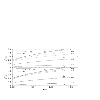
FIG. 2.: Spectra for the four lowest wavefunctions of even parity and $m=0$ (a) for the OBE equation (short-dashed line) and the Bethe-Salpeter equation (solid line), (b) for the OBE+TBE equation (long-dashed line) and the Bethe-Salpeter equation (solid line). The curves are labeled by $n$, which indicates that the curve belongs to the $n^{\text{th}}$ eigenvector. The curve for the $1s$ state for the Bethe-Salpeter equation and the curve for the first OBE+TBE wavefunction are very close together, but distinct.

We plot both the OBE spectra [in Fig. 2(a)] and the OBE+TBE spectra [in Fig. 2(b)] along with the Bethe-Salpeter spectra for the even parity and $m=0$ states. Based on the energies, we see that the $n=1$ state is expected to be the $1s$ state, the $n=2$ state the $2s$ state, and the $n=3$ and $n=4$ states the $3s$ or $3d$ states. We see approximate agreement between both of the truncated Hamiltonian results and the Bethe-Salpeter results for lightly-bound systems (where $E\approx 2M$).

Our states are not manifest eigenstates of total angular momentum $J^{2}$. However, if our approximation of the Hamiltonian potential was good enough, we would be able to identify the $n=3$ and $n=4$ states of the light-front Hamiltonian calculation with $3s$ and $3d$ states of the Bethe-Salpeter equation unambiguously. This would determine the angular momentum of the light-front Schrödinger equation wavefunctions. From Fig. 2, we see both that the addition of the TBE potential brings the $n=3$ and $n=4$ states closer to the Bethe-Salpeter results, and that in the lightly-bound region the $n=3$ and $n=4$ states can be identified as $3s$ and $3d$ states. For more deeply-bound states, this identification cannot be made.

An alternative approach to assigning angular momenta labels would be perform a partial-wave decomposition of the wavefunctions in the real angular momentum basis. The wavefunctions could then be labeled by the angular momentum component which is dominant. In light-front dynamics, this is difficult to do since the perpendicular components of the real angular momentum operator ($J_{x}$ and $J_{y}$) are dynamical, which makes the angular momentum operator as complicated as the Hamiltonian. We are encouraged to look for an alternative operator which is easier to use, yet approximates the behavior of the real angular momentum. We shall use the “relative angular momentum”, defined by $\mathchoice{{\hbox{\boldmath$\displaystyle L$}}}{{\hbox{\boldmath$\textstyle L$}}}{{\hbox{\boldmath$\scriptstyle L$}}}{{\hbox{\boldmath$\scriptscriptstyle L$}}}=\mathchoice{{\hbox{\boldmath$\displaystyle x$}}}{{\hbox{\boldmath$\textstyle x$}}}{{\hbox{\boldmath$\scriptstyle x$}}}{{\hbox{\boldmath$\scriptscriptstyle x$}}}\times\mathchoice{{\hbox{\boldmath$\displaystyle k$}}}{{\hbox{\boldmath$\textstyle k$}}}{{\hbox{\boldmath$\scriptstyle k$}}}{{\hbox{\boldmath$\scriptscriptstyle k$}}}$, where the vectors are equal-time three-vectors. The relative momentum $\textstyle k$ is defined by Eq. (37) and $\textstyle x$ is canonically conjugate to $\textstyle k$. The “relative angular momentum” $\textstyle L$ is used to help analyze our solutions, and is not the same as the real angular momentum that can be derived from the Lagrangian using the energy-momentum tensor. However, we will see that the “relative angular momentum” gives results that are expected from the real angular momentum, so our use of the “relative angular momentum” in place of the real one appears to be justified.

A partial-wave decomposition is performed on the wavefunctions (represented in the relative momentum basis) to obtain the radial wavefunctions $R_{l,m}$ for all “relative angular momentum” states $Y_{l,m}$. Since the potential is not manifestly rotationally invariant when written in terms of the relative momentum, our wavefunctions will have support from many different partial waves. Not all partial waves are allowed; only those partial-wave states with the same $J_{3}$ and parity quantum numbers as the wavefunction give non-vanishing radial wavefunctions. We have

$$\langle\mathchoice{{\hbox{\boldmath$\displaystyle k$}}}{{\hbox{\boldmath$\textstyle k$}}}{{\hbox{\boldmath$\scriptstyle k$}}}{{\hbox{\boldmath$\scriptscriptstyle k$}}}|\psi^{n}_{m,p}\rangle = \sum_{l=m}^{\infty}Y_{l}^{m}(\theta,\phi)R^{n,p}_{l,m}(k).$$ (48)

We define the fraction of the wavefunction with “relative angular momentum” $l$ as

$$f^{n}_{l} = \int_{0}^{\infty}dk\,k^{2}\left|R^{n,p}_{l,m}(k)\right|^{2}.$$ (49)

The fractions $f^{n}_{l}$ are a measure of the amount of “relative angular momentum” state $l$ in the $n^{\text{th}}$ eigenfunction.

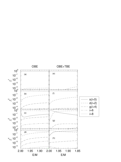
FIG. 3.: These are the fractions of each angular momentum state in the four lowest coupling constant wavefunctions with $m=0$ and even parity plotted as a function of the binding energy $E/M$. The results for the OBE truncation are shown on the left, (a-d), and the OBE+TBE truncation are shown on the right, (e-h). Note that the OBE wavefunctions, in general, have more support from a larger number of partial waves.

To illustrate these “relative angular momentum” fractions, we perform this analysis on the four lowest coupling constant wavefunctions with even parity and $m=0$ for both the OBE and OBE+TBE truncations, the same as in Fig. 2. We show $f^{n}_{l}$ as a function of $E$ in Fig. 3. (The plots for the $m=\pm 1,\pm 2$ states show similar behavior, with different $l$ values.) Note that more higher “relative angular momentum” states contribute for deeper bound states. This is the same behavior that would be expected if the real angular momentum was used to perform the partial wave decomposition. Recall that the real angular momentum will commute with the full potential if no truncation is made. However, the potentials we use are truncated, and neglecting the higher-order terms breaks the rotational invariance of the potential. Also, both the binding and the importance of the higher-order diagrams increase with the coupling constant. Thus, both truncations we consider will break rotational invariance more when the states are more deeply bound. In the absence of having the real angular momentum fractions, we will use the “relative angular momentum” fractions.

Examination of the $f^{n}_{l}$ curves in Fig. 3 shows us that, as postulated earlier, the $n=1$ and $n=2$ states shown in Figs. 3(a,e) and 3(b,f) are predominately $s$-wave states, which we label the $1s$ and $2s$ states respectively. For the OBE truncation, the $n=3$ state shown in Fig. 3(c) is predominately $d$-wave (labeled the $3d$ state) and the $n=4$ state shown in Fig. 3(d) is predominately $s$-wave (labeled the $3s$ state), with little mixing between the two states. For the OBE+TBE truncation, the $n=3$ and $n=4$ states are mixtures of both the $3s$ and $3d$ states, as seen in Figs. 3(g,h) In fact, we see a level crossing between the $n=3,4$ states in that the $n=3$ state is predominantly $3d$ for lightly-bound systems, but as the binding increases, the $n=3$ state becomes predominantly $3s$. Again, this type of mixing would also be found if the real angular momentum was used.

If this $3s$-$3d$ mixing is ignored, then Fig. 3 shows clearly that when the TBE is included the amount of “relative angular momentum” states mixed in actually decreases as compared to the OBE results. This implies that the wavefunctions of the OBE+TBE equation are better “relative angular momentum” states than the wavefunctions of the OBE equation. Thus the TBE potential restores some rotational invariance to the OBE calculation.

We attempt to classify the wavefunctions as states with definite angular momentum. If a wavefunction has the most support from the “relative angular momentum” state $l$, we classify that state as having angular momentum $l$. This procedure designates the first two wavefunctions for both the OBE and the OBE+TBE cases as $s$-wave states, which is clearly the right thing to do. For the third and fourth wavefunctions of the OBE+TBE equation, there are points where the fraction of the $s$-wave state equals the fraction of the $d$-wave state. Here it no longer clear that such a state should be assigned a definite “relative angular momentum” value; we do so regardless and analyze the consequences later.

We now examine the breaking of rotational invariance of the two truncations based on the comparison of states with different $m$ projections of the same angular momentum. Since the $s$-wave state has only $m=0$, there is nothing to analyse in that case. Further discussion of the ground-state $s$-wave will appear in Ref. [7]. In Figs. 4, 5, and 6, we plot the Bethe-Salpeter bound-state spectra along with the spectra for the states constructed with the OBE and the OBE+TBE potentials. The different $m$ states for the Bethe-Salpeter equation are exactly degenerate as a result of the rotational invariance of the equation. The curves from the Hamiltonian theory do not exhibit the exact degeneracy in $m$; the degeneracy is broken whether the OBE or OBE+TBE potentials are used. However, we see that the degeneracy is partially restored when the TBE potential is included, in that for a given binding energy the spread of the coupling constants is always smaller.

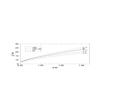
FIG. 4.: Here we plot the curves for the first $p$-wave state, the $2p$ state. The Bethe-Salpeter (BS) result is plotted with a solid line, the OBE results with the short-dashed lines, and the OBE+TBE with the long-dashed lines.

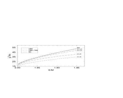
FIG. 5.: Here we plot the curves for the second $p$-wave state, the $3p$ state. The Bethe-Salpeter (BS) result is plotted with a solid line, the OBE results with the short-dashed lines, and the OBE+TBE with the long-dashed lines.

In Figs. 4 and 5, we plot the spectra for the $2p$ and $3p$ states, respectively. In both figures, we see that the $m=0$ and $m=\pm 1$ curves move closer together after addition of the TBE potential. However, the average of the two curves for each case does not move much. In fact, for the $3p$ state in Fig. 5, the $m=\pm 1$ curve moves farther away from the ladder Bethe-Salpeter curve after addition of the TBE. We also note that in Fig. 5 the spread of the spectra is larger than in Fig. 4 for both the OBE and the OBE+TBE light-front Schrödinger equations. We attribute this to the neglect of the higher-order graphs. Since the states with different $m$ values would be degenerate if all the higher-order graphs were included, not including them causes a breaking of the degeneracy. Because the coupling constant is larger for the $3p$ states than for the $2p$ states with the same binding energy, the omission of the higher-order graphs causes a larger breaking of the degeneracy for the $3p$ states.

FIG. 6.: The first $d$-wave state, the $3d$ state. The Bethe-Salpeter (BS) result is plotted with a solid line. In (a) the OBE results are the short-dashed lines, and in (b) the OBE+TBE results are the long-dashed lines. Note that there are two separate $m=0$ curves when the OBE+TBE are used, one extending a quarter of the way over, and the other hiding under the $m=\pm 1$ curve with the OBE+TBE.

We also consider the first $d$-wave states. We see in Fig. 6 that, as in Figs. 4 and 5, the states with different $m$ values move together after addition of TBE. The effect of the level crossing of the $3s$ and $3d$ states shown in Figs. 3(g) and 3(h) is seen here in that there are two disjoint curves for $m=0$. When the level crossing occurs, at $E/M\approx 1.96$, the wavefunction which originally was the $3s$ state becomes the $3d$ state and vice versa.

There are some problems that this level crossing causes. In the intermediate region where the $3s$ and $3d$ states are about equally mixed, it is probably not physically sensible to call the state a $3s$ or $3d$ state. However, plotting the curves gives us an indication of what the wavefunctions are doing, and for this case we see that the $m=0$ curve is always bounded by the $m=\pm 1$ and $m=\pm 2$ curves. A more restrictive classification scheme would leave a gap (in $E/M$) between the two $m=0$ curves and it would not be so clear that the bounding of the $m=0$ curve which we observe here occurs.

Finally, we note that the spread of the curves in the $3d$ case is approximately the same as the spread in the $3p$ case for each truncation. This tells us that the higher-order graphs have the same qualitative effect in both states.

IV Conclusions

In this paper, we considered two truncations of the light-front Hamiltonian, the OBE and OBE+TBE truncations. Using these truncations, a “relative angular momentum” operator was used to study the partial-wave decompositions of the bound-state wavefunctions. We found that the “relative angular momentum” operator acting on those states yield behavior similar to that expected from the real angular momentum. This result encourages the use of this operator to classify the states according to their angular momentum values $l$, and to study the degeneracy of the spectra for states with the same $l$ value but with different projections $m$. We found less breaking of the degeneracy when the OBE+TBE potential was used than when the OBE potential was used. Both of these findings indicate that the OBE+TBE truncation of the Hamiltonian breaks rotational invariance less than the OBE truncation alone.

However, there is still some discrepancy between our truncated Hamiltonian spectra and the ladder Bethe-Salpeter spectra. In general, our OBE+TBE results for the $p$- and $d$-wave states show deeper binding than the Bethe-Salpeter results. Not surprisingly, this disagreement is largest for the most deeply bound-states where the coupling is largest. This difference would be removed if all the higher-order pieces of the potential were included. These higher-order pieces are also needed for the full restoration of rotational invariance.

- [1] P.A. Dirac, Rev. Mod. Phys. 21, 392 (1949).
- [2] S.J. Brodsky, H. Pauli and S.S. Pinsky, Phys. Rept. 301, 299 (1998) hep-ph/9705477.
- [3] G.A. Miller, Phys. Rev. C 56, 2789 (1997) nucl-th/9706028.
- [4] A. Harindranath, hep-ph/9612244.
- [5] T. Heinzl, hep-th/9812190.
- [6] U. Trittmann and H. Pauli, hep-th/9705021.
- [7] J.R. Cooke and G.A. Miller, in preparation.
- [8] N.C. Schoonderwoerd, B.L. Bakker and V.A. Karmanov, Phys. Rev. C 58, 3093 (1998) hep-ph/9806365.
- [9] J.H. Sales, T. Frederico, B.V. Carlson and P.U. Sauer, nucl-th/9909029.
- [10] G.C. Wick, Phys. Rev. 96, 1124 (1954); R.E. Cutkosky, ibid. 96, 1135 (1954).
- [11] Y. Nambu, Prog. Theor. Phys. 5, 614 (1950).
- [12] J. Schwinger, Proc. Nat. Acad. Sci. 37, 452 (1951).
- [13] J. Schwinger, Proc. Nat. Acad. Sci. 37, 455 (1951).
- [14] M. Gell-Mann and F. Low, Phys. Rev. 84, 350 (1951).
- [15] E.E. Salpeter and H.A. Bethe, Phys. Rev. 84, 1232 (1951).
- [16] M.J. Levine, J.A. Tjon, and J. Wright, Phys. Rev. Lett. 16, 962 (1966),
- [17] M.J. Levine, J. Wright, and J.A. Tjon, Phys. Rev. 154, 1433 (1967).
- [18] M.J. Levine and J. Wright, Phys. Rev. D 2, 2509 (1970).
- [19] T. Nieuwenhuis and J.A. Tjon, Phys. Rev. Lett. 77, 814 (1996) hep-ph/9606403.
- [20] A. Klein, Phys. Rev. 90, 1101 (1953).
- [21] D.R. Phillips and S.J. Wallace, Phys. Rev. C 54, 507 (1996) nucl-th/9603008.
- [22] A.D. Lahiff and I.R. Afnan, Phys. Rev. C 56, 2387 (1997) nucl-th/9708037.
- [23] N.E. Ligterink and B.L. Bakker, Phys. Rev. D 52, 5954 (1995) hep-ph/9412315.
- [24] M.V. Terentev, Sov. J. Nucl. Phys. 24, 106 (1976).
- [25] S. Weinberg, Phys. Rev. 150, 1313 (1966).
- [26] A. Paganamenta, in Lectures in Theoretical Physics, Volume XID, edited by K.T. Mahanthappa and W.E. Brittin (Gordon and Breach, New York, 1969), p. 479