Current Conservation in the Covariant
Quark-Diquark Model of the Nucleon

Abstract

The description of baryons as fully relativistic bound states of quark and glue reduces to an effective Bethe-Salpeter equation with quark-exchange interaction when irreducible 3-quark interactions are neglected and separable 2-quark (diquark) correlations are assumed. This covariant quark-diquark model of baryons is studied with the inclusion of the quark substructure of the diquark correlations. In order to maintain electromagnetic current conservation it is then necessary to go beyond the impulse approximation. A conserved current is obtained by including the coupling of the photon to the exchanged quark and direct “seagull” couplings to the diquark structure. Adopting a simple dynamical model of constituent quarks and exploring various parametrisations of scalar diquark correlations, the nucleon Bethe-Salpeter equation is solved and the proton and neutron electromagnetic form factors are calculated numerically. The resulting magnetic moments are still about 50% too small, the improvements necessary to remedy this are discussed. The results obtained in this framework provide an excellent description of the electric form factors (and charge radii) of the proton, up to a photon momentum transfer of 3.5GeV², and the neutron.

1 Introduction

To the precision accessible to current measurements, the proton is the only known hadron that is stable under the effect of all interactions. Protons are thus ideal for use in beams or targets for scattering experiments designed to explore the fundamental dynamics of the strong interaction. From this, it follows that more is known about the proton and its nearly stable isospin partner, the neutron, than any other hadron. There is an abundance of observable properties of the nucleon, from elastic scattering form factors to electromagnetic form factors and parton distributions, which are being measured with increasing precision at various accelerator facilities around the world. In particular, the ratio of the electric and the magnetic form factor of the proton is subject to current measurements at TJNAF, and current experiments at MAMI MAMI and NIKHEF NIKHEF show great promise that soon we will have a precise knowledge of the electromagnetic properties of neutron as well. Hence, the development of an accurate and tractable covariant framework for the nucleon in terms of the underlying quarks and gluons is clearly desirable.

Models of the nucleon and other baryons are numerous and have had varying degrees of success as they are usually designed to describe particular properties of baryons. Some of the frameworks that have been employed are non-relativistic Gel64 ; Kar68 ; Fai68 and relativistic Fey71 quark potential models, bag models Cho74 ; Has78 , skyrmion models Sky61 ; Adk83 ; Schw89 ; Hol93 or the chiral soliton of the Nambu-Jona-Lasinio (NJL) model Alk96a ; Chr96 . The relativistic bound state problem of 3-quark Faddeev type was studied extensively within the NJL model Rei90 ; Buc92 ; Ish93 ; Hua94 ; Buc95 ; Ish95 and its non-local generalization, the global color model Cah89 ; Bur89 . In addition, some complementary aspects of these models have been combined, e.g., the chiral bag model Cho75 ; Rho94 and a hybrid model that implements the NJL-soliton picture of baryons within the quark-diquark Bethe-Salpeter (BS) framework Zue97 .

The present study is concerned with the further development of a description of baryons (and the nucleon, in particular) as bound states of quarks and gluons in a fully-covariant quantum field theoretic framework based on the Dyson-Schwinger equations of QCD. Such a framework has already reached a high level of sophistication for mesons. In these studies, the quark-antiquark scattering kernel is modeled as a confined, non-perturbative gluon exchange. Such a gluon exchange can be provided by solutions to the Dyson-Schwinger equations for the propagators of QCD in the covariant gauge Sme97 ; Sme98 . In phenomenological studies the gross features of such solutions are mimicked by the use of a phenomenological quark-antiquark kernel. With this kernel, the dressed-quark propagator is obtained as the solution of its (quenched) Dyson-Schwinger equation (DSE), and the same kernel is then employed in the quark-antiquark Bethe-Salpeter equation (BSE) from which one obtains the masses of the meson bound states and their BS amplitudes. Once the dressed-quark propagators and meson BS amplitudes have been obtained, observables can be calculated in a straight-forward manner. The success of this approach has been demonstrated in many phenomenological applications, such as electromagnetic form factors Bur96 , decay widths, $\pi$-$\pi$ scattering Rob96 , vector-meson electroproduction Pic97 , to name a few. Summaries of this Dyson-Schwinger/Bethe-Salpeter description of mesons may be found in Refs. Miranski ; Rob94 ; Tan97 .

The significantly more complicated framework required for an analogous description of baryons based on the quantum field theoretic description of bound states in 3-quark correlations has meant that baryons have received far less attention than mesons. Consequently, the utility of such a description for the baryons is considerably less understood, even on the phenomenological level. (For example, the ramifications of various truncation schemes, required in any quantum field theoretic treatment of bound states, which have been explored extensively in the meson sector are completely unknown in the baryon sector.) The developments in this direction employ a picture based on separable 2-quark correlations, i.e., diquarks, interacting with the 3rd quark which allows a treatment of the relativistic bound state in a manner analogous to the 2-body BS problem Kus97 ; Hel97b ; Oet98 . Although these studies employ simplified model assumptions for the quark propagators and diquark correlators, they demonstrate the utility of the approach in general, and these simplified model assumptions can be replaced by more realistic ones in the future as more is understood about the underlying dynamics of quarks and gluons.

In the present article we generalize this framework for the 3-quark bound state problem in quantum field theory to accommodate the quark-substructure of the separable diquark correlations. This necessary extension has important implications on the electromagnetic properties of the nucleons. We explicitly construct a conserved current for their electromagnetic couplings, and we verify analytically that it yields the correct charges of both nucleons. To achieve this we employ Ward and Ward-Takahashi identities for the quark correlations which arise from electromagnetic gauge invariance. In order to avoid unnecessary complications, our present study considers only simple constituent-quark and diquark propagators. However, the generalization to include dressed propagators, most importantly to account for confined nature of quarks and diquarks, requires only minor modifications.

The organization of the article is as follows. In Sec. 2, some general properties of the two-quark correlations (or diquarks) are discussed. The importance of constructing a diquark correlator that is antisymmetric under quark exchange is emphasized. The parametrisations of the Lorentz-scalar isoscalar diquark correlations which are employed in the numerical calculations of the subsequent sections are introduced to reflect these properties in deliberately simple ways. The framework is sufficiently general to accommodate the results for the diquark correlators as they become available from studies of the underlying dynamics of quark and gluon correlations in QCD. Of course, diquark correlations other than the scalar diquark will be important for a more complete description of the nucleon. Certainly necessary is the inclusion of other channels, such as the axialvector diquark, when the description is extended to the octet and the decuplet baryons. Nonetheless, for the purposes of the present study, only scalar diquarks are considered; the generalization to include other diquarks is straight-forward Oet98 . In Sec. 3, the nucleon BS equation and the quark-exchange kernel are introduced. One particular feature of this kernel is that it necessarily depends on the total momentum of the nucleon bound state $P_{n}$. This conclusion is based on general arguments, such as the exchange-antisymmetry of the diquark correlations. It is important to obtain the correct normalizations and charges of the nucleon bound states. In particular, to ensure current conservation requires a considerable extension beyond the impulse approximation in the calculations of electromagnetic form factors for baryons. The numerical solutions for the nucleon BS amplitudes obtained herein preserve the invariance of observables under a re-routing of the relative momentum, a requirement that follows from the translational invariance of the relativistic bound state problem. In Sec. 4, the normalization condition for the nucleon BS amplitude is derived and the nucleon electromagnetic current is obtained in Sec. 5. In Sec. 5.1, the “seagull” contributions to the electromagnetic current, necessary for current conservation, are derived from the Ward and Ward-Takahashi identities. In Sec. 6, expressions for the electromagnetic form factors of the nucleon are derived, the numerical calculations are described in Sec. 6.1, and the results for the form factors are presented and discussed in Sec. 6.2. The conclusions of this study are provided in Sec. 7. Several appendices have also been included with further details which may provide the interested reader with addition insight into the framework.

2 Diquark Correlations

To obtain a solution of the 3-particle Faddeev equations in quantum field theory requires a truncation of the interaction kernel. A widely-employed truncation scheme is to neglect contributions to the Faddeev kernel which arise from irreducible 3-quark interactions. This allows one to rewrite the Dyson series for the 3-quark Green function as a coupled system of equations. The first being the BS equation for the 2-quark scattering amplitude and the other being the Faddeev equation, which describes the coupling of the 3rd quark to these 2-quark correlations. As a result, the nature of the gluonic interactions of quarks enters only in the BSE of the 2-quark subsystem, i.e., in the quark-quark interaction kernel. The solution of the full inhomogeneous BS problem for this 2-quark system is simplified by assuming separable contributions (explained below), hereafter referred to as diquarks, to account for the relevant 2-quark correlations within the hadronic bound state. Herein, a “diquark correlation” thus refers to the use of a separable 4-quark function in the $\bar{3}$ representation of the $SU(3)$ color group. The utility of such diquark correlations for a description of baryon bound states is a central element of the present approach.

While in the NJL model the 2-quark scattering amplitude has the property of being separable, in general this is an additional assumption useful to simplify the 3-quark bound state problem in quantum field theory. An example for separable contributions would be (a finite sum of) isolated poles at timelike total momenta $P^{2}$ of the diquark. Such poles allow the use of homogeneous BSEs to obtain the respective amplitudes from the gluonic interaction kernel of the quarks, and thus to calculate these separable contributions to the 2-quark scattering amplitude.

However, the validity of using a diquark correlator to parametrise the 2-quark correlations phenomenologically, does not rely on the existence of asymptotic diquark states. Rather, the diquark correlator may be devoid of singularities for timelike momenta, which may be interpreted as one possible realization of diquark confinement. In principle, one may appeal to models employing a general, separable diquark correlator which need not have any simple analytic structure, in which case no particle interpretation for the diquark would be possible. The implementation of this model of confined diquark is straight-forward and does not introduce significant changes to the framework. The use of diquark correlations in this capacity is quite general and does not necessarily imply the existence diquarks, which have not been observed experimentally.

The absence of asymptotic-diquark states may be explained in a number of ways. Although, it has been observed that solutions of the BSE in ladder approximation yield asymptotic color-$\bar{3}$ diquark states Pra89 , when terms beyond ladder approximation are maintained, the diquarks cease to be bound Ben96 . That is, the addition of terms beyond the ladder approximation to the BS kernel, in a way which preserves Goldstone’s theorem at every order, has a minimal impact on solutions for the color-singlet meson channels. In contrast, such terms have a significant impact on the color-$\bar{3}$ diquark channels. In Ref. Ben96 , it was demonstrated that these contributions to BS kernel beyond ladder approximation are predominantly repulsive in the color-$\bar{3}$ diquark channel. It was furthermore demonstrated in a simple confining quark model that the strength of these repulsive contributions suffices to move the diquark poles from the timelike $P^{2}$-axis and far into the complex $P^{2}$-plane. While the particular, confining quark model is in conflict with locality, the same effect was later verified within the NJL model Hel97a . This suggests that this mechanism for diquark confinement, which eliminates the possibility of producing asymptotic diquark states, might hold independent of the particular realization of quark confinement.

In a local quantum field theory, on the other hand, colored asymptotic states do exist, for the elementary fields as well as possible colored composites such as the diquarks, but not in the physical subspace of the indefinite metric space of covariant gauge theories. The analytic structure of correlation functions, the holomorphic envelope of extended permuted tubes in coordinate space, is much the same in this description as in quantum field theory with a positive definite inner product (Hilbert) space. In particular, 2-point correlations in momentum space are generally analytic functions in the cut complex $P^{2}$-plane with the cut along the timelike real axis. Confinement is interpreted as the observation that both absorptive as well as anomalous thresholds in hadronic amplitudes are due only to other hadronic states Oeh95 . However, the implementation of this algebraic notion of confinement seems much harder to realize in phenomenological applications.

For the present purposes of developing a general framework for the description of baryon bound states, the question as to whether one should or should not model the diquark correlations in terms of functions with or without singularities for total timelike momentum $P^{2}$ is irrelevant. However, we reiterate that the present framework is able to accommodate both of these descriptions of confinement with only straight-forward modifications.

The goal of the present study is to assess the utility of describing baryons as bound states of quark and diquark correlations, in a framework in which the diquark correlations are assumed to be separable. (The term separable refers to the property that a 4-point Green function $G(p,q;P)$ be independent of the scalar $qp$, where $q$ and $p$ are the relative momenta of the two incoming and outgoing particles, respectively, and $P$ is the total momentum.) To provide a simple demonstration of the general formalism, and its application to the calculation of nucleon form factors, we assume that the diquark correlator corresponds to a single scalar-diquark pole at $P^{2}=m_{s}^{2}$ which is both separable and constituent-like. In this description, the (color-singlet) baryon thus is a bound state of a color-$3$ quark and a color-$\bar{3}$ (scalar) diquark correlation.

Figure 1: The diquark pole in the 4-quark Green function.

Assuming identical quarks, consider the 4-point quark Green function in coordinate space given by

$$G_{\alpha\beta\gamma\delta}(x_{1},x_{2},x_{3},x_{4}) =$$

$$\hskip-28.45274pt\langle T(q_{\gamma}(x_{3})q_{\alpha}(x_{1})\bar{q}_{\beta}(x_{2})\bar{q}_{\delta}(x_{4}))\rangle\;,$$

where $\alpha,\beta,\gamma$, and $\delta$ denote the Dirac indices of the quarks and $T$ denotes time-ordering of the quark fields $q_{\alpha}(x)$. The assumption of a separable diquark correlator, corresponding to the diagram shown in Fig. 1, can be written in momentum space as $G^{\hbox{\tiny sep}}_{\alpha\beta\gamma\delta}(p,q,P)$ where

$$G_{\alpha\gamma,\beta\delta}^{\hbox{\tiny sep}}(p,q,P)\, := e^{-iPY}\,\int d^{4}\!X\,d^{4}\!y\,d^{4}\!z\,\,e^{iqz}e^{-ipy}$$ (2)

$$\hskip 42.67912pte^{iPX}G_{\alpha\beta\gamma\delta}^{\hbox{\tiny sep}}(x_{1},x_{2},x_{3},x_{4})$$

$$= D(P)\;\chi_{\gamma\alpha}(p,P)\bar{\chi}_{\beta\delta}(q,P)\;\;,$$

where $D(P)$ is the diquark propagator, $X=\sigma x_{1}+(1\!-\!\sigma)x_{3}$, $Y=(1\!-\!\sigma^{\prime})x_{2}+\sigma^{\prime}x_{4}$, the total momentum partitioning of the outgoing and incoming quark pairs are given respectively by $\sigma$ and $\sigma^{\prime}$ both in $[0,1]$, and $y=x_{1}-x_{3}$, $z=x_{2}-x_{4}$.

As described above, the separable form of the diquark correlation of Eq. (2) does not necessarily entail the existence of an asymptotic diquark state. The framework developed herein makes no restrictions on the particular choice of the diquark propagator $D(P)$. Technically, model correlations which mimic confinement through the absence of timelike poles are easy to implement as shown in Ref. Hel97b .

Nonetheless, for the purpose of demonstration, here we employ the simplest form for this propagator corresponding to a simple (scalar) diquark bound state in the 2-quark Green function $G$ of Eq. (2). The appearance of such an asymptotic diquark state requires the diquark propagator to have a simple pole at $P^{2}=m_{s}^{2}$, where $m_{s}$ is the mass of the diquark bound state, i.e.,

$$D(P)=\frac{i}{P^{2}-m_{s}^{2}+i\epsilon}\;.$$ (3)

Then $\chi(p,P)$ and its adjoint $\bar{\chi}(p,P)=\gamma_{0}\chi^{\dagger}(p,P)\gamma_{0}$ are the BS wave functions of the (scalar) diquark bound state which are defined as the matrix elements of two quark fields or two antiquark fields between the bound state and the vacuum, respectively. Further details concerning these definitions are given in Appendix A.

It is convenient to define the truncated diquark BS amplitudes (sometimes referred to as BS vertex functions) $\widetilde{\chi}$ and $\widetilde{\bar{\chi}}$ from the BS wave functions in Eq. (2) by amputating the external quark propagators,

$$\widetilde{\chi}(p,P) := S^{-1}((1\!-\!\sigma)P+p)\;\chi(p,P)\;{S^{-1}}^{T}\!(\sigma P-p)\,,$$ (4)

$$\widetilde{\bar{\chi}}(p,P) := {S^{-1}}^{T}\!(\sigma P-p)\;\bar{\chi}(p,P)\;S^{-1}((1\!-\!\sigma)P+p)\,.$$ (5)

The convention employed here is to use the same symbols for both the BS wave functions and the truncated BS amplitudes, with the latter denoted by a tilde. An important observation made in Appendix A, which is of use in the following discussions, is that the for identical quarks, antisymmetry under quark exchange constrains the diquark BS amplitudes $\widetilde{\chi}$ to satisfy:

$$\widetilde{\chi}(p,P)\,=\,\left.-\widetilde{\chi}^{T}(-p,P)\right|_{\sigma\leftrightarrow(1-\sigma)}\!.$$ (6)

Note that $\sigma$ and $(1\!-\!\sigma)$ have been interchanged here.

In principle, at this point one could go ahead and specify the form of the kernel for the quark-quark BSE in ladder approximation, and obtain diquark BS amplitudes in much the same manner in which solutions for the mesons are obtained. However, as discussed above, the appearance of stable bound state solutions might be an artifact of the ladder approximation rather than the true nature of the quark-quark scattering amplitude. Therefore, for our present purposes various simple model parametrisations for diquark BS amplitudes are explored, rather than using a particular solution of the diquark homogeneous BSE. The motivation is to explore the general aspects and implications of using a separable diquark correlation for the description of the nucleon bound state.

For separable contributions of the pole type (3), but possibly complex mass (with Re$(m_{s}^{2})>0$), one readily obtains standard BS normalization conditions to fix the overall strength of the quark-quark coupling to the diquark for a given parametrisation of the diquark structure. These are obtained from the inhomogeneous quark-quark BSE for the Green function of Eq. (2) employing pole dominance for $P^{2}$ sufficiently close to $m_{s}^{2}$. To sketch their derivation consider the inhomogeneous BSE which is of the general form,

$$G(p,q,P)\,=\,\left({G^{(0)}}^{-1}(p,q,P)-K(p,q,P)\right)^{-1}\;.$$ (7)

Here $G^{(0)}$ denotes the antisymmetric Green function for the disconnected propagation of two identical quarks. The definition of its inverse ${G^{(0)}}^{-1}$ and a brief discussion of how to derive it, may be found in Appendix A. With the simplifying assumption that the quark-quark interaction kernel $K$ be independent on the total diquark momentum $P$; that is, $K(p,q,P)\equiv K(p,q)$ (which is satisfied in the ladder approximation for example), the derivative of $G$ with respect to the total momentum $P$, gives the relation

$$-P^{\mu}\frac{\partial}{\partial P^{\mu}}\,G(p,q,P)\,=\,\int\frac{d^{4}k}{(2\pi)^{4}}\frac{d^{4}k^{\prime}}{(2\pi)^{4}}$$ (8)

$$\hskip 17.07182ptG(p,k,P)\left(P^{\mu}\frac{\partial}{\partial P^{\mu}}\,{G^{(0)}}^{-1}\!(k,k^{\prime},P)\right)G(k^{\prime},q,P)\;.$$

Upon substitution of $G(p,q,P)$ as given by Eqs. (2) and (3), and equating the residues of the most singular terms, one obtains the non-linear constraint for the normalization of the diquark BS amplitudes $\chi$ and $\bar{\chi}$,

$$1 \,\stackrel{{\scriptstyle!}}{{=}}\, \frac{-i}{4m_{s}^{2}}\int\frac{d^{4}p}{(2\pi)^{4}}$$

$$\left\{\hbox{tr}\left(S^{T}(p_{\beta})\widetilde{\bar{\chi}}(p,P)\left(P\frac{\partial}{\partial P}S(p_{\alpha})\right)\widetilde{\chi}(p,P)\right)\right.$$

$$\hskip 14.22636pt+\,\left.\hbox{tr}\left(\widetilde{\bar{\chi}}(p,P)S(p_{\alpha})\widetilde{\chi}(p,P)\left(P\frac{\partial}{\partial P}S^{T}(p_{\beta})\right)\right)\right\}\;,$$

where $p_{\alpha}=p+(1\!-\!\sigma)P$ and $p_{\beta}=-p+\sigma P$, i.e., $P=p_{\alpha}+p_{\beta}$ and $p=\sigma p_{\alpha}-(1\!-\!\sigma)p_{\beta}$. The scalar diquark contribution, relevant to the present study of the nucleon bound state, is color-$\bar{3}$ and isosinglet. Lorentz covariance requires its Dirac structure to be the sum of four independent contributions, each proportional to a function of two independent momenta. For simplicity only a single term is maintained here, which has the following structure:

$$\widetilde{\chi}(p,P)=\gamma_{5}C\,\frac{1}{N_{s}}\tilde{P}(p^{2},pP)\;,$$ (10)

where $C$ is the charge conjugation matrix ($C=i\gamma_{2}\gamma_{0}$ in the standard representation). The normalization constant $N_{s}$ is fixed from the condition given in Eq. (2) for a given form of $\tilde{P}(p^{2},pP)$.

It may seem reasonable to neglect the dependence of this invariant function on the scalar $pP$; such a simplification would yield the leading moment of an expansion of the angular dependence in terms of orthogonal polynomials, which has been shown to provide the dominant contribution to the meson bound state amplitudes in many circumstances. However, in the present case the antisymmetry of the diquark wave function, c.f., Eqs. (6), entails that

$$\tilde{P}(p^{2},pP)\,=\,\left.\tilde{P}(p^{2},-pP)\right|_{\sigma\leftrightarrow(1-\sigma)}\;.$$ (11)

For $\sigma\not=1/2$ and thus for $\bar{p}:=p\big{|}_{\sigma\leftrightarrow(1-\sigma)}\not=p$, it is not possible to neglect the $pP$ dependence in the amplitude without violating the quark-exchange antisymmetry. To maintain the correct quark-exchange antisymmetry, we assume instead that the amplitude depends on both scalars, $p^{2}$ and $pP$ in a specific way. In particular, we assume the diquark BS amplitude is given by a function that depends on the scalar

$$x := p_{\alpha}p_{\beta}-\sigma(1-\sigma)\,m_{s}^{2}=-(1-2\sigma)pP-p^{2}$$ (12)

$$= (1-2\sigma)\bar{p}P-\bar{p}^{2}$$

with $\bar{p}=(1-\sigma)p_{\alpha}-\sigma p_{\beta}$ and $p_{\{\alpha,\beta\}}$ as given above. For equal momentum partitioning between the quarks in the diquark correlation $\sigma=1/2$, the scalar $x$ reduces to the negative square of the relative momentum, $x=-p^{2}$. The two scalars that may be constructed from the available momenta $p$ and $P$ (noting that $P^{2}=m^{2}_{s}$ is fixed) which have definite symmetries under quark exchange are given by the two independent combinations $p_{\alpha}p_{\beta}$ (which is essentially the same as above $x$) and $p_{\alpha}^{2}-p_{\beta}^{2}$. The latter may only appear in odd powers which are associated with higher moments of the BS amplitude. Hence, these are neglected by setting

$$\tilde{P}(p^{2},pP)\equiv P(x)$$ (13)

which can be shown to satisfy the antisymmetry constraint given by Eq. (11) $\forall\sigma\in[0,1]$. Finally, the diquark BS normalization $N_{s}$, as obtained from Eq. (2), is given by

$$N_{s}^{2}\, = \,\frac{-i}{4m_{s}^{2}}\int\frac{d^{4}p}{(2\pi)^{4}}\;P^{2}(x)$$

$$\hskip 28.45274ptP\frac{\partial}{\partial P}\;\hbox{tr}\big{[}S(p+(1\!-\!\sigma)P)S(-p+\sigma P)\big{]}\;.$$

The numerical results presented in the following sections explore the ramifications of several Ansätze for $P(x)$,

$$P_{n\mbox{\tiny-P}}(x)=\left(\frac{\gamma_{n}}{x+\gamma_{n}}\right)^{n}\hskip-2.84544pt\mbox{or}\;P_{\hbox{\tiny EXP}}(x)=\exp\,\{-x/\gamma_{\hbox{\tiny EXP}}\},$$ (15)

where the integer $n=1,2...$ and corresponds to monopole, dipole,… diquark BS amplitudes. Their widths $\gamma_{n}$, $\gamma_{\hbox{\tiny EXP}}$ are determined from the nucleon BSE by varying them until the diquark normalization given by Eq. (2) and coupling strength $g_{s}^{2}$ necessary to produce the correct nucleon bound-state mass are equal. This is carried out numerically and described in detail in Sec. 3.

For completeness, various Gaussian forms that peak for values of $x=x_{0}\geq 0$,

$$P_{\hbox{\tiny GAU}}(x)\,=\,\exp\,\{-(x-x_{0})^{2}/\gamma_{\hbox{\tiny GAU}}^{2}\}\;,$$ (16)

are also explored. Such forms with finite $x_{0}$ were suggested for diquark amplitudes as a result of a variational calculation of an approximate diquark BSE in Ref. Pra88 and have been used in the nucleon calculations of Ref. Bur89 . Therein, a fit to the Gaussian form given by Ref. Pra88 (and Eq. (16) above) was employed with a width of $\gamma_{\hbox{\tiny GAU}}\simeq 0.11$GeV² and $x_{0}/\gamma_{\hbox{\tiny GAU}}\simeq 1.7$. From a calculation within the present framework, which is described in Sec. 3, we observe that the necessary value for $\gamma_{\hbox{\tiny GAU}}$ to obtain a reasonable nucleon mass is about an order of magnitude smaller than the value given in Ref. Bur89 . Furthermore in Sec. 6, we observe that the effect of a finite $x_{0}$ on the electric form factor of the neutron rules out the use of a Gaussian form with $x_{0}\not=0$.

Some of the parametrisations used for diquark correlations in previous quark-diquark model studies of the nucleon Kus97 ; Hel97b ; Oet98 , correspond to neglecting the substructure of diquarks entirely; this may be reproduced in the present framework by setting $\tilde{P}(p^{2},pP)=1$. By neglecting the diquark substructure, the diquark BS normalizations such as $N_{s}$ here are not well-defined. The strengths of the quark-diquark couplings are undetermined and chosen as free adjustable parameters of the model (one for each diquark channel maintained). In the present, more general approach, these couplings are determined by the normalizations of the respective diquark amplitudes. At present this is the scalar diquark normalization $N_{s}$ alone which in turn determines the coupling strength $g_{s}=1/N_{s}$ between the quark and diquark which binds the nucleon.

The aim of our present study is to generalize the notion of diquark correlations by going beyond the use of a point-like diquark and include a diquark substructure in a form similar to that of mesons. In the most general calculation of the three-body bound state, the strength of the quark-diquark coupling is not at one’s disposal; it arises from the elementary interactions between the quarks. By using the diquark BS normalization condition of Eq. (2), we can assess whether the quark-diquark picture of the nucleon is still able to provide a reasonable description of the nucleon bound state if the coupling strength is obtained from the diquark BSE rather than forcing the quark and diquark to bind by adjusting their couplings freely. Whether the quark-diquark coupling is sufficiently strong to produce bound baryons will eventually be determined by the strength of the quark-quark interaction kernel that leads to the diquark BS amplitude.

Finally, the use of a diquark BS amplitude with a finite width improves on the previous calculations in yet another respect. Without the substructure of the diquark, an additional ultraviolet regularization had to be introduced in the exchange kernel of the BSE for the nucleon in Refs. Kus97 ; Hel97b ; Oet98 . In the present study, the finite-sized substructure of the diquark leads to a nucleon BSE which is completely regular in the ultraviolet in a natural way.

In this section, we have discussed some general features of the diquark amplitude employed in our present study. The important observations are the implications of its antisymmetry under quark exchange which constrains the functional dependence on the quark momenta, and the derivation of the BS normalization condition, Eq. (2), to fix the quark-diquark coupling strength. By taking these into account, we will find that the precise form of the Ansatz for the diquark BS amplitude $P(x)$ has little qualitative influence on the resulting nucleon amplitudes as long as $P(x)$ falls off by at least one power of $x$ for large $x$ corresponding to a large spacelike relative momentum.

3 The Quark-Diquark Bethe-Salpeter Equation of the Nucleon

By neglecting irreducible 3-quark interactions in the kernel of the Faddeev equation giving the 6-point Green function that describes the fully-interacting propagation of 3 quarks, the Dyson series for this 6-point Green function reduces to a coupled set of two-body Bethe-Salpeter equations, see for example, Ref. Hua94 . As discussed in the previous section, for the purpose of demonstrating the framework developed herein, we choose to employ constituent quark and diquark propagators. However, the framework itself is much more general. The assumptions under which it is developed require only that the irreducible 3-quark interactions are neglected in the nucleon Faddeev kernel and that the diquark correlations be well-parametrised by a sum of separable terms (which may or may not have poles associated with asymptotic diquark states).

Maintaining only the (flavor-singlet, color-$\bar{3}$) scalar diquark channel in these correlations, corresponding to Eqs. (2) and (3), the appearance of a stable nucleon bound state coincides with the development of a pole in the Green function $G_{\alpha\beta}$ describing the fully-interacting (spin-${1}/{2}$) quark and (scalar) diquark correlations which is of the form,

$$G^{\hbox{\tiny pole}}_{\alpha\beta}(p,k,P_{n}) =$$

$$\left(\psi(p,P_{n})\frac{i(P\kern-5.0pt/_{n}+M_{n})}{P_{n}^{2}-M_{n}^{2}+i\epsilon}\bar{\psi}(-k,P_{n})\right)_{\alpha\beta}.$$

Here $k$ and $p$ are the relative momenta between the quark and diquark, incoming and outgoing, respectively, $P_{n}$ is the four-momentum of the nucleon with mass $M_{n}$, $\alpha$ and $\beta$ denote the Dirac indices of the quark, and the nucleon BS wave function $\psi(p,P_{n})$ is related to it’s adjoint according to

$$\bar{\psi}(p,P_{n})\,=\,\gamma_{0}\psi^{\dagger}(-p,P_{n})\gamma_{0}\,=\,C\psi^{T}(p,-P_{n})C^{-1}\,.$$ (18)

The truncated nucleon BS amplitude $\widetilde{\psi}$ is defined as

$$\psi(p,P_{n})=D((1\!-\!\eta)P_{n}-p)S(\eta P_{n}+p)\widetilde{\psi}(p,P_{n})\;,$$ (19)

where $\eta\in[0,1]$ is the fraction of the nucleon momentum $P_{n}$ carried by the quark. The resulting homogeneous Bethe-Salpeter equation for the nucleon bound state reads,

$$\widetilde{\psi}_{\alpha\beta}(p,P_{n})=\int\frac{d^{4}k}{(2\pi)^{4}}\;K_{\alpha\gamma}(p,k;P_{n})\,\psi_{\gamma\beta}(k,P_{n})\;,$$ (20)

where $K_{\alpha\beta}(p,k;P_{n})$ is the kernel of the nucleon BSE which represents the exchange of one of the quarks within the diquark with the spectator quark. Maintaining the quark-exchange antisymmetry of the diquark correlations, this kernel provides the full antisymmetry within the nucleon (i.e., Pauli’s principle) in the quark-diquark model Rei90 .

$\scriptstyle p\,=\,(1\!-\!\eta)p_{\alpha}-\eta(q+p_{\beta})\;,\quad k\,=\,(1\!-\!\eta)p_{\beta}-\eta(q+p_{\alpha})$.

Figure 2: The quark-exchange kernel of the nucleon BSE.

The exchange kernel is shown in Fig. 2 and given by

$$K_{\alpha\beta}(p,k;P_{n})\, =$$

$$\hskip-28.45274pt\,-\frac{1}{2}\,\widetilde{\chi}_{\alpha\gamma}(p_{1},q+p_{\alpha})\,S^{T}_{\gamma\delta}(q)\,\widetilde{\bar{\chi}}^{T}_{\delta\beta}(p_{2},q+p_{\beta})$$

$$= \,\frac{1}{2N_{s}^{2}}\,P(x_{1})P(x_{2})\;S_{\alpha\beta}(q)\;,$$ (22)

where the factor -1/2 arises from the flavor coupling between the quark and diquark and $p_{1}$ and $p_{2}$ are the relative momenta of the quarks within the incoming and outgoing diquark, respectively, such that

$$p_{1}=\sigma p_{\alpha}-(1\!-\!\sigma)q\;,\quad\hbox{and}\quad p_{2}=(1\!-\!\sigma^{\prime})q-\sigma^{\prime}p_{\beta}\;.$$ (23)

The respective momentum partitionings are $\sigma$ and $\sigma^{\prime}$ and need not be equal. The total momenta of the incoming and the outgoing diquark are $q+p_{\alpha}$ and $q+p_{\beta}$. The momentum $q$ of the exchanged quark is expressed in terms of the total nucleon momentum $P_{n}$ and relative momenta $k$ and $p$ as

$$q\,=\,(1\!-\!2\eta)P_{n}-p-k\;.$$ (24)

Using the definitions of $q$ and the quark momenta $p_{\alpha}=\eta P_{n}+p$ and $p_{\beta}=\eta P_{n}+k$, the relative momenta in the diquark BS amplitudes can be expressed as

$$p_{1}\, = \,(\sigma\eta-(1\!-\!\sigma)(1\!-\!2\eta))P_{n}+(1\!-\!\sigma)k+p\;,$$ (25)

$$p_{2}\, = \,((1\!-\!\sigma^{\prime})(1\!-\!2\eta)-\sigma^{\prime}\eta)P_{n}-k-(1\!-\!\sigma^{\prime})p\;.$$ (26)

The corresponding arguments of the quark-exchange-antisymmetric diquark BS amplitudes follow readily from their definition in Eq. (12),

$$x_{1}\, = \,-p_{1}^{2}-(1\!-\!2\sigma)((1\!-\!\eta)p_{1}P_{n}-p_{1}k)\;,$$ (27)

$$x_{2}\, = \,-p_{2}^{2}+(1\!-\!2\sigma^{\prime})((1\!-\!\eta)p_{2}P_{n}-p_{2}p)\;.$$ (28)

Before proceeding, it is worth summarizing some of the important aspects of this framework:

1. The dependence of the exchange kernel on the total nucleon bound-state momentum $P_{n}$ is crucial in order to obtain the correct relationship between the electromagnetic charges of the proton and neutron bound states and the normalizations of their BS amplitudes.

2. The momentum $q$ of the exchanged quark is independent of the nucleon momentum $P_{n}$ only for the particular value of momentum partitioning $\eta=1/2$.

3. The relative momenta $p_{1}$ and $p_{2}$ of the quarks within the diquarks are only independent of the total momentum $P_{n}$ of the nucleon for the particular choice:

   $$\sigma=\sigma^{\prime}=\frac{1-2\eta}{1-\eta}\;.$$ (29)

   The symmetric arguments of $x_{1}$ and $x_{2}$ in the diquark BS amplitudes are independent of the total momentum $P_{n}$ only if, in addition to the above criteria, $\sigma=\sigma^{\prime}=1/2$ as well, and hence $\eta=1/3$. In fact, this conclusion can be further generalized: Any exchange-symmetric argument of the diquark amplitude can differ from the definition of Eq. (12) only by a term that is proportional to the square of the total diquark momentum. From this, it is possible to show that the diquark BS amplitudes can be independent of $P_{n}$ only if $\eta=1/3$. This is shown in Appendix B.

Unlike the ladder-approximate kernels commonly employed in phenomenological studies of the meson BSE, the quark-exchange kernels of the BSEs for baryon bound states, such as the one depicted in Fig. 2, necessarily depend on the total momentum of the baryon $P_{n}$ for all values of $\eta\in[0,1]$. This has important implications on the normalization of the bound-state BS amplitudes as well as on the calculation of the electromagnetic charges of the bound states. In particular, considerable extensions of the framework beyond the impulse approximation are required in the calculation of electromagnetic form factors in order to ensure that the electromagnetic current is conserved for baryons. This issue is explored in detail in Sec. 5.

The form of the pole contribution arising from the nucleon bound state to the quark-diquark 4-point correlation function in Eq. (3) constrains the nucleon BS amplitude to obey the identities:

$$\widetilde{\psi}(p,P_{n})\Lambda^{+}(P_{n}) = \widetilde{\psi}(p,P_{n})\;,$$ (30)

$$\Lambda^{+}(P_{n})\widetilde{\bar{\psi}}(p,P_{n}) = \widetilde{\bar{\psi}}(p,P_{n})\;,$$ (31)

where $\Lambda^{+}(P_{n})\,=\,(P\kern-5.0pt/_{n}+M_{n})/2M_{n}$. It follows from this that the most general Lorentz-covariant form of the nucleon BS amplitude can be parametrised by

$$\widetilde{\psi}(p,P_{n})\, =$$

$$\hskip-42.67912ptS_{1}(p,P_{n})\,\Lambda^{+}(P_{n})\,+\,S_{2}(p,P_{n})\,\Xi(p,P_{n})\,\Lambda^{+}(P_{n})\;,$$

$$\widetilde{\bar{\psi}}(p,P_{n})\, =$$

$$\hskip-42.67912ptS_{1}(-p,P_{n})\,\Lambda^{+}(P_{n})\,+\,S_{2}(-p,P_{n})\,\Lambda^{+}(P_{n})\,\Xi(-p,P_{n})\;,$$

where $\Xi(p,P_{n})=(p\kern-5.0pt/-pP_{n}/M_{n})/M_{n}$, and $S_{1}(p,P_{n})$ and $S_{2}(p,P_{n})$ are Lorentz-invariant functions of $p$ and $P_{n}$. This provides a separation of the positive and negative energy components of the nucleon BS amplitude. In Appendix B, some of the consequences of this decomposition are explored. In particular, it allows one to rewrite the homogeneous BSE of Eq. (20) in a compact manner, in terms of a 2-vector $S^{T}(p,P_{n}):=(S_{1}(p,P_{n}),\,S_{2}(p,P_{n}))$ as

$$S(p,P_{n}) =$$

$$\hskip-34.14322pt\frac{1}{2N_{s}^{2}}\int\frac{d^{4}k}{(2\pi)^{4}}\;P(x_{1})P(x_{2})\,D(k_{s})\,T(p,k,P_{n})\,S(k,P_{n})\;,$$

where $k_{s}=(1\!-\!\eta)P_{n}-k\,$ and $T(p,k,P_{n})$ is a $2\times 2$ matrix in which each of the four elements is given by a trace over the Dirac indices of the quark propagator $S(k_{q})$ (with $k_{q}=\eta P_{n}+k$), the propagator $S(q)$ of the exchanged quark and a particular combination of Dirac structures derived from the decomposition of the nucleon amplitude in Eq. (3), see Appendix B.

  

Figure 3: The first 5 moments of the nucleon BS amplitudes $S_{1}$ (left) and $S_{2}$ (right).

Upon carrying out these traces, the resulting BSE is transformed into the Euclidean metric by introducing 4-dimensional polar coordinates corresponding to the rest frame of the nucleon according to the following prescriptions (where “$\to$” denotes the formal transition from the Minkowski to the Euclidean metric):

$$p^{2}\,\to\,-p^{2}\;,\quad P_{n}^{2}\to M_{n}^{2}\;,\quad pP_{n}\,\to\,iM_{n}p\,y\;,$$ (35)

$$\mbox{and}\quad S(p,P_{n})\,\to\,S(p,y)\;.$$

Written in terms of these variables, the nucleon BS amplitude is a function of the square of the relative momentum $p^{2}$ and the cosine $y\in[-1,+1]$ of the azimuthal angle between the four-vectors $p$ and $P_{n}$. The dependence of the nucleon BS amplitudes $S(p,y)$ on the angular variable $y$ is approximated by an expansion to the order $N$ in terms of the complete set of Chebyshev polynomials $T_{n}(y)$,

$$S(p,y)\, \simeq \,\sum_{n=0}^{N-1}(-i)^{n}\,S_{n}(p)T_{n}(y)$$ (36)

$$S_{n}(p) = i^{n}\,\frac{2}{N}\sum_{k=1}^{N}S(p,y_{k})T_{n}(y_{k})\;,$$ (37)

$$\hbox{where}\;y_{k} = \cos\left(\frac{\pi(k-1/2)}{N}\right)$$

are the zeros of the Chebyshev polynomial $T_{N}(y)$ of degree $N$ in $y$. Here, we employ Chebyshev polynomials of the first kind with a convenient (albeit non-standard) normalization for the zeroth Chebyshev moment from setting $T_{0}=1/\sqrt{2}$. The explicit factor of $(-i)^{n}$ is introduced into Eq. (36) to ensure that the moments $S_{n}(p)$ are real functions of positive $p\equiv\sqrt{p^{2}}$ for all $n$. The BSE for these moments of the nucleon BS amplitude is then

$$S_{m}(p) =$$

$$\,-\frac{1}{2N_{s}^{2}}\,\int\frac{k^{3}dk}{(4\pi)^{2}}\,\sum_{n=0}^{N-1}\,i^{m-n}\;T_{mn}(p,k)\,S_{n}(k)\;,$$

where the ($2N\times 2N$) matrix $T_{mn}(p,k)$ is obtained from $T(p,k,P_{n})$ by expanding in terms of Chebyshev polynomials both amplitudes $S$ in the nucleon BSE of Eq. (3); that is, summing over the $y_{k}$ on both sides of Eq. (3) according to Eq. (37) and using Eq. (36) for the BS amplitude on the right-hand side. The definition of the matrix $T_{mn}$ appearing in Eq. (3) furthermore includes the explicit diquark propagator and BS amplitudes $P(x_{1})$ and $P(x_{2})$ of the integrand in Eq. (3) as well as the integrations over all angular variables. Its exact form is provided in Appendix B.

Figure 4: Dependence of $\lambda/N_{s}^{2}$ on $\eta$ for fixed $\sigma=\sigma^{\prime}=1/2$ (solid) and with $\sigma$, $\sigma^{\prime}$ from Eq. (29) (dashed). The width $\gamma_{2}$ is fixed to yield $\lambda/N_{s}^{2}=1$ at $\eta=1/3$.

In the calculations presented herein, we restrict ourselves to the use of free propagators for constituent quark and diquark, with masses $m_{q}$ and $m_{s}$ respectively, as the simplest model to parametrise the quark and diquark correlations within the nucleon. Measuring all momenta in units of the nucleon bound-state mass $M_{n}$ leaves $m_{q}/M_{n}$ and $m_{s}/M_{n}$ as the only free parameters. Using for the scalar diquark amplitude $P(x)$ the forms of Eqs. (15) or (16) with fixed widths $\gamma$, the homogeneous BSE for the nucleon in Eq. (20) is converted into an eigenvalue equation of the form,

$$\lambda\,\widetilde{\psi}(p,P_{n})\,=\,\int\frac{d^{4}k}{(2\pi)^{4}}\;N_{s}^{2}K(p,k,P_{n})\,\psi(p,P_{n})\;,$$ (39)

with the additional constraint that $\lambda=N_{s}^{2}$ (note that $N_{s}^{2}K$ is independent of $N_{s}$). This equation is solved iteratively and the largest eigenvalue $\lambda$ is found which corresponds to the nucleon ground-state. To implement the constraint, we calculate the diquark normalization $N_{s}^{2}$ from Eq. (2) and compare it to the eigenvalue $\lambda$. This procedure is repeated with a new value for the width $\gamma$ of the diquark BS amplitude until the eigenvalue obtained from the BSE agrees with the normalization integral in Eq. (2); that is, until the constraint $\lambda=N_{s}^{2}$ is satisfied.

A typical solution of the nucleon BSE is shown in Fig. 3. Five orders were retained in the Chebyshev expansion. The figure depicts the relative importance of the first four Chebyshev moments of the nucleon amplitudes $S_{1}(p,P_{n})$ and $S_{2}(p,P_{n})$. The respective results for their fifth moments are too small ($\leq 10^{-4}$) to be distinguished from zero on the scale of Fig. 3. This provides an indication for the high accuracy obtained from the Chebyshev expansion to this order. This particular solution, which will be shown to provide a good description of the electric form factors in Sec. 6, was obtained for the dipole form of the diquark amplitude, i.e., from Eq. (15) with $n=2$, using $m_{q}=0.62M_{n}$ and $m_{s}=0.7M_{n}$ (with $\sigma=\sigma^{\prime}=1/2$, $\eta=1/3$). The value for the corresponding diquark width $\gamma_{2}$, necessary to yield $\lambda=N_{s}^{2}$ (to an accuracy of $10^{-3}$), resulted thereby to be $\gamma_{2}=(0.294\,M_{n})^{2}$.

The dependence of the BS eigenvalue on the momentum partitioning parameter $\eta$ is shown in Fig. 4. The complex domains of the constituent quark and diquark momentum variables, $k_{q}^{2}$ and $k_{s}^{2}$ respectively, that are sampled by the integration over the relative momentum $k$ in the nucleon BSE are devoid of poles for $1-m_{s}/M_{n}<\eta<m_{q}/M_{n}$. The pole in the momentum $q^{2}$ of the exchanged quark of the kernel in Eq. (22) is avoided by imposing the further bound $\eta>(1-m_{q}/M_{n})/2$ on the momentum partitioning parameter. Therefore, with the present choice of constituent masses it is for values of $\eta$ in the range $0.3<\eta<0.6$, for which our numerical methods can yield stable results.

In principle, the integrations necessary to solve the nucleon BSE should always be real and never lead to an imaginary result (since $m_{q}+m_{s}>M_{n}$). More refined numerical methods would be necessary, however, when integrations were to be performed in presence of the poles in the constituent propagators that occur within the integration domain for values of $\eta$ outside the above limits.

  

Figure 5: The leading moments of the nucleon BS amplitudes $S_{1}$ (left) and $S_{2}$ (right) for the diquark amplitudes (15,16) with $m_{q}$ adjusted to yield $S_{1,0}(p)|_{p=0.2M_{n}}=1/2$.

The momentum partitioning within the nucleon $\eta$ is not an observable. Hence, for any value of $\eta$ for which our numerical results are stable, we expect the eigenvalue of the nucleon BSE $\lambda$ (which implicitly determines the nucleon mass) to be independent of $\eta$. In Fig. 4, the dependence on $\eta$ of the nucleon BSE eigenvalue $\lambda$ is explored using a fixed value for $\sigma=\sigma^{\prime}=1/2$ (solid curve) and using the values of $\sigma$ and $\sigma^{\prime}$ from Eq. (29) (dashed curve).

In the first case, the arguments of the diquark amplitudes simplify to $x_{i}=-p_{i}^{2}$ with $p_{1}=-(1\!-\!3\eta)P_{n}/2+p+k/2$ and $p_{2}=(1\!-\!3\eta)P_{n}/2-k-p/2$. This implies that the real parts of $x_{i}$ are guaranteed to be positive only for $\eta=1/3$. For values of $\eta\not=1/3$, a negative contribution arises from the timelike nucleon bound-state momentum $P_{n}$. If the $n$-pole forms for the diquark amplitudes are employed, this results in the appearance of artificial poles whenever $(1\!-\!3\eta)^{2}M_{n}^{2}/4\geq\gamma_{n}$. The value of $\gamma_{2}=(0.294\,M_{n})^{2}$ as it results here, would entail the appearance of a pole for $\eta\geq 0.53$. This explains why our numerical procedure becomes unstable as $\eta$ approaches the value $1/2$ in this case.

No such timelike contribution to the $x_{i}$ arises in the second case shown in Fig. 4. Here, for $\sigma=\sigma^{\prime}=(1\!-\!2\eta)/(1\!-\!\eta)$ the relative momenta $p_{i}$ are independent of $P_{n}$, and there are no terms $\propto M_{n}^{2}$ in $x_{i}$; see, for example, Eqs. (27,28). However, as $\eta\to 1/2$, we find that $\sigma,\sigma^{\prime}\to 0$ and the diquark normalization integrals are then affected by singularities.

Fixed width $S_{1}(p)|_{p=0.2M_{n}}=1/2$, see Fig. 5:
$P(x)$	$m_{s}\;[M_{n}]$	$m_{q}\;[M_{n}]$	$\sqrt{\gamma}\;[M_{n}]$	$g_{s}=1/N_{s}$
$n=1$	0.7	0.685	0.162	117.1
$n=2$	0.7	0.620	0.294	91.80
$n=4$	0.7	0.605	0.458	85.47
$n=6$	0.7	0.600	0.574	84.37
$n=8$	0.7	0.598	0.671	83.76
EXP	0.7	0.593	0.246	82.16
GAU	0.7	0.572	0.238	71.47
Fixed masses, see Fig. 6:
$n=1$	0.7	0.62	0.113	155.8
$n=2$	0.7	0.62	0.294	91.80
$n=4$	0.7	0.62	0.495	81.08
$n=6$	0.7	0.62	0.637	78.61
EXP	0.7	0.62	0.283	74.71

Table 1: Summary of parameters used for the various diquark amplitudes $P(x)$, c.f., Eqs. (15,16).

In the restricted range allowed to $\eta$, the results for the nucleon BSE obtained herein are found to be independent of $\eta$ to very good accuracy when the equal momentum partitioning between the quark in the diquarks is used, $\sigma=\sigma^{\prime}=1/2$. In this case, the diquark normalization in Eq. (2) yields a fixed value for $N^{2}_{s}$ and any $\eta$ dependence of the ratio $\lambda/N_{s}^{2}$ has to arise entirely from the nucleon BSE. The $\eta$ independence of $\lambda$ thus demonstrates that the solutions to the nucleon BSE are under good control.

The more considerable $\eta$-dependence observed for $\sigma=\sigma^{\prime}=(1\!-\!2\eta)/(1\!-\!\eta)$ arises from the dependence of $N_{s}^{2}$ on $\sigma$, $\sigma^{\prime}$. Here, the limitations of the model assumptions for the diquark BS amplitudes are manifest. The dependence of the diquark BS amplitudes on the diquark bound-state mass, higher Chebyshev moments (which have been neglected) and the Lorentz structures (which we have neglected), are all responsible for this observed $\sigma$ dependence. Such a dependence would not occur, had the diquark amplitudes employed herein been calculated from the diquark BSE.

For the numerical calculations of electromagnetic form factors presented in Sec. 5, we therefore choose to restrict the model to $\sigma=\sigma^{\prime}=1/2$ and vary $\eta$. From the observed independence of the nucleon BSE solutions to $\eta$ (when $\sigma=\sigma^{\prime}=1/2$), one expects to find that calculated nucleon observables, such as the electromagnetic form factors, will display a similar independence of $\eta$ as well.

  

Figure 6: The moments $S_{1,0}$ (left) and $S_{2,0}$ (right) of the nucleon amplitudes for the diquark amplitudes of Eqs. (15,16) with fixed masses, $m_{s}=0.7M_{n}$, $m_{q}=0.62M_{n}$.

In Figure 5 the zeroth Chebyshev moments $S_{1,0}(p)$ and $S_{2,0}(p)$ obtained from a numerical solution of the nucleon BSE with $\sigma=\sigma^{\prime}=1/2$ and $\eta=1/3$ are shown, for various diquark amplitudes of the forms given in Eqs. (15) and Eq. (16) with $x_{0}=0$. To provide a comparison between these different forms of diquark BS amplitude, we have chosen to keep the diquark mass fixed and vary the quark mass until a solution of the nucleon BSE was found with the property that

$$S_{1,0}(p)|_{p=0.2M_{n}}\stackrel{{\scriptstyle!}}{{=}}1/2\;.$$ (40)

The resulting values for $m_{q}$ along with the corresponding diquark widths and couplings $g_{s}\equiv 1/N_{s}$ are summarized in Table 1.

We observe that the mass of the quark required to satisfy the condition in Eq. (40) tends to smaller values for higher $n$-pole diquark amplitudes. On the other hand, for fixed constituent quark (and diquark) mass the higher $n$-pole diquark amplitudes lead to wider nucleon amplitudes. This is shown in Fig. 6 and the corresponding diquark widths and couplings are given in the lower part of Table 1. The mass values hereby correspond to the results shown in the previous Figure 5 for $n=2$.

The qualitative effect of shifting the maximum in the Gaussian forms in Eq. (16) for the diquark amplitudes by a finite amount $x_{0}$, is shown in Fig. 7. The curve for $x_{0}=0$ resembles the Gaussian result given in Fig. 5 with masses $m_{s}=0.7M_{n}$ and $m_{q}=0.572M_{n}$, which are kept fixed in the results for finite shifts $x_{0}$. The corresponding widths and normalizations of these forms for the diquark amplitudes are given in Table 2. While the widths $\gamma$ and the couplings $g_{s}$ are not free parameters in our approach, the additional parameter $x_{0}/\gamma_{\hbox{\tiny GAU}}$ introduced into the form of the diquark BS amplitude is free to vary. In contrast to the Gaussian form of the model diquark BS amplitude employed in Ref. Bur89 with $x_{0}/\gamma_{\hbox{\tiny GAU}}=0.19/0.11\simeq 1.73$, by implementing the diquark normalization condition, we find that the width must be about 30 times smaller to provide a sufficient interaction strength $g_{s}=1/N_{s}^{2}$ necessary to bind the nucleon.

To provide for a closer comparison with the results of Ref. Bur89 , we have also solved the nucleon BSE using the values of parameters employed in that study. That is, we have solved the nucleon BSE using $P_{\hbox{\tiny GAU}}(x)$ with the parameter $x_{0}/\gamma_{\hbox{\tiny GAU}}=0.19/0.11$ and using the constituent quark and diquark masses $m_{q}=0.555M_{n}$ and $m_{s}=0.7M_{n}$, respectively. (Note that we use the nucleon mass as the intrinsic momentum scale of our framework, whereas the momentum scale employed in Ref. Bur89 was 1 GeV.) The value employed in Ref. Bur89 for the diquark mass $m_{s}=$ 0.568 GeV implies that $M_{n}=$ 811 MeV in order to compare to our calculations (with $m_{s}=0.7M_{n}$), and our value for the quark mass ($m_{q}=0.555M_{n}$) thus corresponds to $m_{q}=$ 0.45 GeV. With these parameters, we obtain $\gamma_{\hbox{\tiny GAU}}=(0.216\,M_{n})^{2}=$ $0.308\,10^{-2}\mbox{GeV}^{2}$, which may be compared to $\gamma_{\hbox{\tiny GAU}}=(0.409\,M_{n})^{2}=0.11\,\mbox{GeV}^{2}$ used in Ref. Bur89 .

  

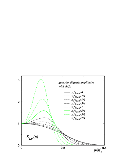
Figure 7: The moment $S_{1,0}$ for the Gaussian diquark amplitudes of Eq. (16) with various shifts $x_{0}/\gamma_{\mbox{\tiny GAU}}$ (left), see Table 2, and a comparison (right) of our result for $x_{0}/\gamma_{\mbox{\tiny GAU}}=19/11$ (with $m_{s}=0.7M_{n}$, $m_{q}=0.555M_{n}$) with a result we obtain from using $\gamma_{\mbox{\tiny GAU}}=0.11$GeV² as in Ref. Bur89 .

$m_{s}=0.7M_{n}$, $m_{q}=0.572M_{n}$:
$x_{0}/\gamma_{\hbox{\tiny GAU}}$	$\sqrt{\gamma_{\hbox{\tiny GAU}}}\;[M_{n}]$	$g_{s}=1/N_{s}$
0	0.238	71.47
1/4	0.209	69.09
1/2	0.181	72.64
3/4	0.154	81.96
1	0.130	97.75
5/4	0.109	121.3
3/2	0.091	154.3
7/4	0.077	198.5

Table 2: Width and normalizations of Gaussian amplitudes, Eq. (16) for various shifts $x_{0}$, see Fig. 7 (right).

The same results for the nucleon amplitudes as shown above are used for the calculations of the electromagnetic form factors of the proton and the neutron in Sec. 6. We will show that when $n$-pole diquark BS amplitudes with $n=2$ and $n=4$ are employed, one obtains results for the electromagnetic form factors that are in good agreement with the phenomenological dipole fit for the electric proton form factor, while higher powers or exponential forms tend to produce form factors which decrease too fast with increasing momentum transfer $Q^{2}$. We also show that use of a Gaussian form for the diquark BS amplitude with $x_{0}\not=0$ leads to neutron electric form factor that has a qualitatively different behavior than that obtained by using the other model forms of diquark BS amplitudes. Furthermore, this form leads to nodes in the neutron electric form factor for small $Q^{2}$, a feature for which there is no experimental evidence.

4 Normalization of Nucleon Bethe-Salpeter Amplitude

In order to reproduce the correct electromagnetic charges of the physical asymptotic states, it is required that their Bethe-Salpeter (or Faddeev) amplitudes be normalized according to the normalization conditions obtained from the fully-interacting Green functions of the elementary fields. These normalization conditions are derived from inhomogeneous BS (or Faddeev) equations. In the present framework, the quark-diquark 4-point Green function is given by (suppressing Dirac indices)

$$G(p,q,P)\,=\,\left({G^{(0)}}^{-1}(p,q,P)-K(p,q,P)\right)^{-1}\;.$$ (41)

Here, $K(p,q,P)$ is the quark-exchange kernel of Eq. (22) depicted in Fig. 2, and $G^{(0)}(p,q,P)$ is the disconnected contribution to this Green function, given by

$$G^{(0)}_{\alpha\beta}(p,k,P)\,:=\,(2\pi)^{4}\delta^{4}(p-k)\,S_{\alpha\beta}(k_{q})\,D(k_{s})\delta_{\eta\eta^{\prime}}\;,$$ (42)

with $k_{q}=\eta P+k$ and $k_{s}=(1\!-\!\eta)P-k$. Taking the derivative of $G(p,k,P)$ with respect to the total momentum $P$ and then examining the leading contributions in the limit that $P^{2}\rightarrow M_{n}^{2}$ which arise from the nucleon pole contribution from Eq. (3), one finds

$$M_{n}\,\Lambda^{+}(P_{n}) \stackrel{{\scriptstyle!}}{{=}} \;i\int\frac{d^{4}p}{(2\pi)^{4}}\frac{d^{4}k}{(2\pi)^{4}}$$

$$\hskip-34.14322pt\bar{\psi}(-p,P_{n})\left(P_{\mu}\frac{\partial}{\partial P_{\mu}}G^{-1}(p,k,P)\right)_{P=P_{n}}\!\psi(k,P_{n})\;.$$

The most important difference in normalizing the amplitudes in the Bethe-Salpeter framework developed here and a genuine two-body BSE, is the dependence of the BS kernel on the total momentum of the bound-state $P$. In phenomenological studies of 2-body bound states BS kernels, such as ladder-approximate ones for example, are most commonly employed in a form which does not depend on the bound-state momentum. However, in the present approach, the original 3-body nature of the nucleon bound state requires the exchange kernel of the reduced BS equation for quark and diquark to depend on the total momentum $P_{n}$ of the nucleon. In particular, when $\eta\not=1/2$, the propagator for the exchanged quark in the kernel depends on the total momentum $P_{n}$ and for $\eta\not=1/3$, the diquark BS amplitudes depend on $P_{n}$. This added complication, which is easily avoided by ladder-approximate studies of meson bound states is unavoidable for studies of baryons. Thus, the normalization condition for the nucleon will always contain contributions from the derivative of the kernel.

Following the above procedure, one obtains a normalization condition of the form

$$1\, \stackrel{{\scriptstyle!}}{{=}}$$

$$\hskip-2.84544pt\eta N_{q}+(1-\eta)N_{D}+(1-2\eta)N_{X}+(1-3\eta)N_{P}\;,$$

where

$$N_{q}\, = \,-\frac{P^{\mu}}{2M_{n}}i\int\frac{d^{4}k}{(2\pi)^{4}}\;D(k_{s})$$

$$\hskip 56.9055pt\hbox{tr}\bigg{[}\widetilde{\bar{\psi}}(-k,P)\left(\frac{\partial}{\partial k_{q}^{\mu}}S(k_{q})\right)\widetilde{\psi}(k,P)\bigg{]}\;,$$

$$N_{D}\, = \,-\frac{P^{\mu}}{2M_{n}}i\int\frac{d^{4}k}{(2\pi)^{4}}\;\left(\frac{\partial}{\partial k_{s}^{\mu}}D(k_{s})\right)$$

$$\hskip 85.35826pt\hbox{tr}\bigg{[}\widetilde{\bar{\psi}}(-k,P)S(k_{q})\widetilde{\psi}(k,P)\bigg{]}\;,$$

$$N_{X}\, = \,-\frac{P^{\mu}}{2M_{n}}i\int\frac{d^{4}p}{(2\pi)^{4}}\frac{d^{4}k}{(2\pi)^{4}}\;\frac{1}{2N_{s}^{2}}\,P(-p^{2}_{1})P(-p^{2}_{2})$$

$$\hskip 56.9055pt\hbox{tr}\bigg{[}\bar{\psi}(-p,P)\left(\frac{\partial}{\partial q^{\mu}}S(q)\right)\psi(k,P)\bigg{]}\;,$$

$$N_{P}\, = \,-\frac{P^{\mu}}{2M_{n}}i\int\frac{d^{4}p}{(2\pi)^{4}}\frac{d^{4}k}{(2\pi)^{4}}\;\frac{1}{2N_{s}^{2}}$$

$$\hskip 14.22636pt\bigg{(}\,p_{1\mu}\,P^{\prime}(-p^{2}_{1})P(-p^{2}_{2})\,-\,p_{2\mu}\,P(-p^{2}_{1})P^{\prime}(-p^{2}_{2})\,\bigg{)}$$

$$\hskip 85.35826pt\hbox{tr}\bigg{[}\bar{\psi}(-p,P)S(q)\psi(k,P)\bigg{]}\;,$$

with $p_{1}=-(1\!-\!3\eta)P/2+p+k/2\,,\;p_{2}=(1\!-\!3\eta)P/2-p/2-k\,,\;\mbox{for}\;\sigma\!=\!\sigma^{\prime}\!=\!1/2$.

It is clear from Eq. (4) that either the exchanged quark or the presence of a diquark substructure, or in general both, provide non-vanishing contributions to the nucleon BS normalization. Maintaining these terms is critical for the correct determination of the electromagnetic charges of baryons since the nucleon normalization and electromagnetic form factors are intimately related by the differential Ward identities.

In the following section, we show that in calculations of the electromagnetic form factors of the nucleon, use of the usual impulse approximation Man55 (which includes only contributions arising from the coupling of the photon to the quark and diquark, that are related to the terms $N_{q}$ and $N_{D}$ in the normalization condition), by itself is insufficient to guarantee electromagnetic current and charge conservation of the nucleon.

One of the additional contributions required for the proper calculation of electromagnetic form factors that goes beyond the usual impulse approximation is the coupling of the photon to the exchanged-quark in the kernel from Eq. (3). We will show that this term provides a crucial contribution to the nucleon electromagnetic form factors and helps maintain electromagnetic current conservation of the nucleon. It is interesting to note that the contribution of this term is important even in the special case that $\eta=1/2$ in which the term $N_{X}$ does not contribute to the normalization condition of Eq. (4).

We will show in the next section that in the presence of a diquark with a non-trivial substructure, additional, direct couplings of the photon to this substructure are required to maintain current conservation. Similar contributions have previously been found important in several other contexts Oth89 ; Wan96 . These couplings are commonly referred to as “seagulls”.

We conclude this section by summarizing that the respective contributions to the nucleon normalization condition of Eq. (4) given in Eqs. (4) to (4) correspond to the usual impulse approximate contributions arising from the constituent quark and diquark, plus the contribution from the exchange-quark in the BS kernel, and the seagull contributions which arise from the quark-substructure in the diquark correlations.

5 The Electromagnetic Current in Impulse Approximation and Beyond

The electromagnetic current operator $J^{\hbox{\tiny em}}_{\mu}(x)$ in impulse approximation is determined by the disconnected contributions from the electromagnetic couplings of the spectator quark ($J^{\mu}_{q}$) and the scalar diquark ($J^{\mu}_{D}$) which in the Mandelstam formalism are calculated from the following momentum space kernels Man55 ,

$$J^{\mu}_{q}(p,P^{\prime};k,P)\, = \,(2\pi)^{4}\delta^{4}(p-k-\hat{\eta}Q)$$

$$\hskip-28.45274ptq_{q}\,\Gamma^{\mu}_{q}(\eta P^{\prime}+p,\eta P+k)\;D^{-1}(\hat{\eta}P-k)\;,$$

$$J^{\mu}_{D}(p,P^{\prime};k,P)\, = \,(2\pi)^{4}\delta^{4}(p-k+\eta Q)$$

$$\hskip-28.45274ptq_{D}\,\Gamma^{\mu}_{D}(\hat{\eta}P^{\prime}-p,\hat{\eta}P-k)\;S^{-1}(\eta P+k)\;,$$

with $Q=P^{\prime}-P$ and $\eta+\hat{\eta}=1$. The charge of the spectator quark in the nucleon is denoted $q_{q}$, the charge of the scalar diquark is $q_{D}$, and $q_{q}+q_{D}=$ 1 and 0 for the proton and neutron, respectively. The Ward-Takahashi identities for the quark and diquark electromagnetic vertices are

$$Q_{\mu}\Gamma^{\mu}_{q}(p+Q,p)\, = \,iS^{-1}(p+Q)\,-\,iS^{-1}(p)\;,$$ (51)

$$Q_{\mu}\Gamma^{\mu}_{D}(p+Q,p)\, = \,iD^{-1}(p+Q)\,-\,iD^{-1}(p)\;.$$ (52)

From these one can immediately write down the nucleon matrix elements for the divergences of the corresponding Mandelstam currents between initial and final nucleon states with momentum and spin $P,\,s$ and $P^{\prime},\,s^{\prime}$ respectively, as

$$\langle P^{\prime},s^{\prime}|\partial_{\mu}J^{\mu}_{q}(0)|P,s\rangle = \,q_{q}\int\frac{d^{4}k}{(2\pi)^{4}}\,\Big{\{}$$

$$\hskip-71.13188pt\bar{u}(P^{\prime},s^{\prime})\,\widetilde{\bar{\psi}}(-(k+\hat{\eta}Q),P^{\prime})\psi(k,P)\,u(P,s)$$

$$\hskip-56.9055pt-\,\bar{u}(P^{\prime},s^{\prime})\,\bar{\psi}(-(k+\hat{\eta}Q),P^{\prime})\widetilde{\psi}(k,P)\,u(P,s)\Big{\}},$$

$$\langle P^{\prime},s^{\prime}|\partial_{\mu}J^{\mu}_{D}(0)|P,s\rangle = \,q_{D}\int\frac{d^{4}k}{(2\pi)^{4}}\,\Big{\{}$$

$$\hskip-71.13188pt\bar{u}(P^{\prime},s^{\prime})\,\widetilde{\bar{\psi}}(-(k-\eta Q),P^{\prime})\psi(k,P)\,u(P,s)$$

$$\hskip-56.9055pt-\,\bar{u}(P^{\prime},s^{\prime})\,\bar{\psi}(-(k-\eta Q),P^{\prime})\widetilde{\psi}(k,P)\,u(P,s)\Big{\}}\;.$$

Here, we insert the BSEs for the amplitudes $\widetilde{\psi}$ and $\widetilde{\bar{\psi}}$ which can be written in the compact form,

$$\widetilde{\psi}(p,P) = \int\frac{d^{4}k}{(2\pi)^{4}}\,K(p,k,P)\,\psi(p,P)\;,$$ (55)

$$\widetilde{\bar{\psi}}(-p,P) = \int\frac{d^{4}k}{(2\pi)^{4}}\,\bar{\psi}(-k,P)\,K(p,k,P)\;.$$ (56)

After shifting the integration momentum by $p+\hat{\eta}Q\to p$ in the second terms of Eqs. (5) and (5), one obtains,

$$\langle P^{\prime},s^{\prime}|\partial_{\mu}J^{\mu}_{q}(0)|P,s\rangle\, = \,q_{q}\int\frac{d^{4}p}{(2\pi)^{4}}\frac{d^{4}k}{(2\pi)^{4}}\,\Big{\{}$$

$$\hskip-99.58464pt\bar{u}(P^{\prime},s^{\prime})\,\bar{\psi}(-p,P^{\prime})K(p,k+\hat{\eta}Q,P^{\prime})\psi(k,P)\,u(P,s)$$

$$\hskip-91.04872pt-\,\bar{u}(P^{\prime},s^{\prime})\,\bar{\psi}(-p,P^{\prime})K(p-\hat{\eta}Q,k,P)\psi(k,P)\,u(P,s)\Big{\}}\;,$$

$$\langle P^{\prime},s^{\prime}|\partial_{\mu}J^{\mu}_{D}(0)|P,s\rangle\, = \,q_{D}\int\frac{d^{4}p}{(2\pi)^{4}}\frac{d^{4}k}{(2\pi)^{4}}\,\Big{\{}$$

$$\hskip-99.58464pt\bar{u}(P^{\prime},s^{\prime})\,\bar{\psi}(-p,P^{\prime})K(p,k-\eta Q,P^{\prime})\psi(k,P)\,u(P,s)$$

$$\hskip-91.04872pt-\,\bar{u}(P^{\prime},s^{\prime})\,\bar{\psi}(-p,P^{\prime})K(p+\eta Q,k,P)\psi(k,P)\,u(P,s)\Big{\}}\;.$$

Examination of the terms in Eqs. (5) and (5) reveals that their sum gives rise to a conserved current only if $K(p,k,P)$ $\equiv K(p-k)$. That is, if the nucleon BS kernel is independent of the total nucleon bound-state momentum $P$ and, in addition, it only depends on the difference of the relative momenta $p-k$. These criteria are satisfied in studies of meson bound states within the ladder approximation, see for example Ref. Tan97 . However, we observe that even in absence of an explicit dependence on the total nucleon momentum $P$, the exchange kernel of the BSE, as obtained from the nucleon Faddeev equation, necessarily depends on the sum of the relative momenta $p+k$ and not their difference. It follows that even with approximating the exchange kernel by a $P$-independent one, which corresponds to neglecting diquark substructure together with using $\eta=1/2$ as in Refs. Hel97b ; Oet98 , the electromagnetic current of the nucleon is not conserved in the impulse approximation and it is already necessary to include an additional coupling of the photon to the quark-exchange kernel.

It is interesting to note that similar photon-kernel couplings are required in other systems as well. For example, while the nucleon-nucleon scattering kernels due to meson exchanges depend only on the difference of the relative momenta (i.e., $K\equiv K(p-k)$), the isospin dependence of a charged meson that is exchanged between the two nucleons requires one to introduce additional photon couplings to the exchanged meson to maintain current conservation, in this case the charged pion. Such contributions play an important role in determining the electromagnetic form factors of the deuteron Gro87 . For the importance of meson-exchange currents in few-nucleon systems, see also the recent review, Ref. Car98 .

The coupling of the exchange quark (with electromagnetic charge $q_{X}$) in the kernel of Eq. (3) gives rise to the additional contribution $J_{X}$ to the nucleon current:

$$\hskip-25.6073ptJ^{\mu}_{X}(p,P^{\prime};k,P)\,=\,\hbox{\hfill}\,-q_{X}\,\frac{1}{2}$$

$$\hskip-14.22636pt\widetilde{\chi}(p_{1},\hat{\eta}P-k)\,S^{T}(q)\,{\Gamma^{\mu}_{q}}^{T}(q^{\prime},q)\,S^{T}(q^{\prime})\,\widetilde{\bar{\chi}}^{T}(p_{2}^{\prime},\hat{\eta}P^{\prime}-p)\;,$$

with $$q\,=\,\hat{\eta}P-\eta P^{\prime}-p-k\;,\;\;q^{\prime}\,=\,q+Q\;,$$

$$\hskip-25.6073ptp_{1}\,=\,\sigma(\eta P^{\prime}+p)-\hat{\sigma}q\;,\;\;p_{2}^{\prime}\,=\,-\sigma^{\prime}(\eta P+k)+\hat{\sigma}^{\prime}q^{\prime}\;,$$

and $$\sigma+\hat{\sigma}=\sigma^{\prime}+\hat{\sigma}^{\prime}=1\;.$$

From the Ward-Takahashi identity for the quark-photon vertex in Eq. (51), one finds that the divergence of the exchanged-quark contribution to the nucleon electromagnetic current is

$$Q_{\mu}J^{\mu}_{X}(p,P^{\prime};k,P)\, =$$

$$\hskip-71.13188pt\,-iq_{X}\,\frac{1}{2}\,\biggl{(}\widetilde{\chi}(p_{1},\hat{\eta}P-k)\,S^{T}(q)\,\widetilde{\bar{\chi}}^{T}(p_{2}^{\prime},\hat{\eta}P^{\prime}-p)$$

$$\hskip-28.45274pt-\,\widetilde{\chi}(p_{1},\hat{\eta}P-k)\,S^{T}(q^{\prime})\,\widetilde{\bar{\chi}}^{T}(p_{2}^{\prime},\hat{\eta}P^{\prime}-p)\,\biggr{)}\;.$$

To provide a comparison with the quark and diquark electromagnetic currents given above for the quark-exchange kernel of Eq. (3) written using the same momentum conventions as used in Eq. (5), we rewrite the divergences of the Mandelstam currents given in Eqs. (5) and (5) as

$$Q_{\mu}J^{\mu}_{q}(p,P^{\prime};k,P)\, =$$

$$\hskip-85.35826pt\,-iq_{q}\,\frac{1}{2}\,\biggl{(}\widetilde{\chi}(p_{1},\hat{\eta}P-k)\,S^{T}(q)\,\widetilde{\bar{\chi}}^{T}(p_{2}^{\prime}-Q,\hat{\eta}P^{\prime}-p)$$

$$\hskip-56.9055pt-\,\widetilde{\chi}(p_{1}-Q,\hat{\eta}P-k)\,S^{T}(q^{\prime})\,\widetilde{\bar{\chi}}^{T}(p_{2}^{\prime},\hat{\eta}P^{\prime}-p)\,\biggr{)}\;,$$

$$Q_{\mu}J^{\mu}_{D}(p,P^{\prime};k,P)\, =$$

$$\hskip-85.35826pt\,-iq_{D}\,\frac{1}{2}\,\biggl{(}\widetilde{\chi}(p_{1}-\hat{\sigma}Q,\hat{\eta}P-k+Q)\,S^{T}(q^{\prime})\,\widetilde{\bar{\chi}}^{T}(p_{2}^{\prime},\hat{\eta}P^{\prime}-p)$$

$$\hskip-71.13188pt-\,\widetilde{\chi}(p_{1},\hat{\eta}P-k)\,S^{T}(q)\,\widetilde{\bar{\chi}}^{T}(p_{2}^{\prime}-\hat{\sigma}^{\prime}Q,\hat{\eta}P^{\prime}-p-Q)\,\biggr{)}\;.$$

Since $q_{q}\,-\,q_{D}\,+\,q_{X}\,=\,0$, one thus finds that, in the case of a point-like diquark BS amplitude, (i.e., neglecting any momentum dependence in the diquark BS amplitudes $\widetilde{\chi}$ and $\widetilde{\bar{\chi}}$), the sum of the three currents given above now yields a conserved electromagnetic current for the nucleon; that is,

$$Q_{\mu}\,\biggl{(}J^{\mu}_{q}\,+\,J^{\mu}_{D}\,+\,J^{\mu}_{X}\biggr{)}\,=\,0\;.$$ (63)

For this cancellation all three contributions are crucial. In particular, the contributions from the photon coupling to the exchanged quark $J^{\mu}_{X}$, as well as the impulse approximate contributions $J^{\mu}_{q}\,+\,J^{\mu}_{D}$ must all be included. For the quark-diquark model of baryons, these three contributions to the current correspond to those given in Ref. Bla99a for the general structure of the one-particle contributions to the current of a 3-particle Faddeev bound state (when the interactions are due to a separable 2-particle scattering kernel). In the NJL model the one-particle contributions yield the complete current of the 3-particle bound state Ish95 .

However, if the substructure of the diquark BS amplitudes is taken into account and the diquark BS amplitude is dependent on any momentum, the cancellation of the longitudinal pieces in the one-particle contributions, Eqs. (5) to (5), is destroyed. Additional photon couplings which are not of the one-particle type become necessary. The violations to current conservation from the one-particle contributions can be displayed in the present framework in a way which will become useful in following sections. Rearranging the six terms from the Eqs. (5), (5) and (5) in such a way as to factor out two terms,

$$S_{1}(p,P^{\prime};k,P)\, := \,-iq_{q}\,\widetilde{\chi}(p_{1}-Q,\hat{\eta}P-k)\,+$$

$$\hskip-56.9055ptiq_{D}\,\widetilde{\chi}(p_{1}-\hat{\sigma}Q,\hat{\eta}P-k+Q)\,-\,iq_{X}\,\widetilde{\chi}(p_{1},\hat{\eta}P-k)\;,$$

$$S_{2}(p,P^{\prime};k,P)\, := \,-iq_{q}\,\widetilde{\bar{\chi}}(p_{2}^{\prime}-Q,\hat{\eta}P^{\prime}-p)\,+$$

$$\hskip-56.9055ptiq_{D}\,\widetilde{\bar{\chi}}(p_{2}^{\prime}-\hat{\sigma}^{\prime}Q,\hat{\eta}P^{\prime}-p-Q)\,-\,iq_{X}\,\widetilde{\bar{\chi}}(p_{2}^{\prime},\hat{\eta}P^{\prime}-p)\;,$$

one obtains

$$Q_{\mu}\,\biggl{(}J^{\mu}_{q}\,+\,J^{\mu}_{D}\,+\,J^{\mu}_{X}\biggr{)}\, =$$

$$\hskip-71.13188pt-\frac{1}{2}\biggl{(}S_{1}(p,P^{\prime};k,P)S^{T}(q^{\prime})\,\widetilde{\bar{\chi}}^{T}(p_{2}^{\prime},\hat{\eta}P^{\prime}-p)$$

$$\hskip-56.9055pt-\,\widetilde{\chi}(p_{1},\hat{\eta}P-k)\,S^{T}(q)\,S_{2}^{T}(p,P^{\prime};k,P)\,\biggr{)}\;.$$

It will be demonstrated in the subsection below that these contributions are exactly canceled by the so-called “seagull” contributions which arise from one-particle irreducible 4-point couplings of the two quarks, the diquark and photon. Such terms must be included whenever the substructure of a diquark bound state (in form of a momentum-dependent diquark BS amplitude) is included in the description of the nucleon. Analogous seagull contributions were previously found necessary in $\gamma$-meson-baryon-baryon couplings to satisfy the corresponding Ward-Takahashi identities Oth89 ; Wan96 .

Note that terms analogous to the explicit one-particle contributions to the bound state currents presented in this section can also be obtained by employing a “generalized” impulse approximation for the 3-particle Faddeev amplitudes. This procedure was recently adopted in an exploratory study of the electromagnetic nucleon form factors Blo99 . In this study five distinct (one-particle) contributions to the form factors arose which were calculated using parameterizations of a simplified nucleon Faddeev amplitude. From the separable-kernel Faddeev equation one readily verifies, however, that only three of these five contributions are independent. These three have the exact same topology as the one-particle contributions presented above. Starting from the generalized impulse approximation, the relative weights of these contributions differ, however, from those needed for current conservation. The latter can be systematically derived from a gauging technique Ish98 . The discrepancy in the weights is due to an overcounting of the (generalized) impulse approximation which can therefore not lead to a conserved current Bla99b . This problem is independent of the necessity for the additional seagull contributions which persists when non-pointlike diquarks are used. We will now address these contributions.

5.1 Ward Identities and Seagulls

The Ward-Takahashi identity for the quark-photon vertex, Eq. (51), follows from the equal-time commutation relation for the electromagnetic quark-current operator $j_{\mu}(x)$ with the quark field (with charge $q_{q}$),

$$\ [j^{0}(x),q(y)]\,\delta(x_{0}-y_{0})\,=\,-q_{q}\,q(x)\,\delta^{4}(x-y)\;,$$

$$\ [j^{0}(x),\bar{q}(y)]\,\delta(x_{0}-y_{0})\,=\,q_{q}\,\bar{q}(x)\,\delta^{4}(x-y)\;.$$ (67)

Formal problems with equal-time commutation relations for interacting fields can be avoided by replacing the canonical formalism with a Lagrangian formulation based on relativistic causality rather than to single out a sharp timelike surface Pei52 . However, as an operational device for the derivation of Ward identities, the equal-time commutation relations of Eqs. (67) will nevertheless give the correct result.

Consider the 5-point Green function that describes the photon coupling to four quarks $G^{\mu}_{\alpha\gamma,\beta\delta}$. Using the notation that $q_{q\alpha}$, $q_{q\beta}$, $q_{q\gamma}$, and $q_{q\delta}$ denote the charges of the quark fields with Dirac indices denoted by $\alpha$, $\beta$, $\gamma$ and $\delta$, respectively, the Ward identity is given by

$$\hskip-5.69046pt\partial_{\mu}^{z}\,\langle T\big{(}q_{\gamma}(x_{3})q_{\alpha}(x_{1})\bar{q}_{\beta}(x_{2})\bar{q}_{\delta}(x_{4})\,j^{\mu}(z)\big{)}\rangle\,=$$ (68)

$$\hskip 2.84544pt-\,\big{(}\,q_{q\alpha}\,\delta^{4}(x_{1}-z)\,+\,q_{q\gamma}\,\delta^{4}(x_{3}-z)-\,q_{q\beta}\,\delta^{4}(x_{2}-z)\,$$

$$\hskip 28.45274pt-\,q_{q\delta}\,\delta^{4}(x_{4}-z)\,\big{)}\;\langle T\big{(}q_{\gamma}(x_{3})q_{\alpha}(x_{1})\bar{q}_{\beta}(x_{2})\bar{q}_{\delta}(x_{4})\big{)}\rangle\;.$$

The 4-point function on the right-hand side has the diquark pole contribution given in Eq. (2) and depicted in Fig. 1. The Fourier transformation of the left-hand side of Eq. (68) allows one to define,

$$G^{\mu}_{\alpha\gamma,\beta\delta}(p,P^{\prime};k,P)\, :=$$

$$\hskip-56.9055pt\int d^{4}\!x_{1}\,d^{4}\!x_{2}\,d^{4}\!x_{3}\,d^{4}\!x_{4}\,\;e^{ip_{\alpha}x_{1}}\,e^{ip_{\beta}x_{2}}\,e^{ip_{\gamma}x_{3}}\,e^{ip_{\delta}x_{4}}$$

$$\hskip-17.07182pt\langle T\big{(}q_{\gamma}(x_{3})q_{\alpha}(x_{1})\bar{q}_{\beta}(x_{2})\bar{q}_{\delta}(x_{4})\,j^{\mu}(0)\big{)}\rangle\;.$$

Here, $p=\sigma p_{\gamma}-\hat{\sigma}p_{\alpha}$, $k=\sigma^{\prime}p_{\beta}-\hat{\sigma}^{\prime}p_{\delta}$ and $P^{\prime}=P+Q$ as before. It is straight forward to verify the following Ward identity for this 5-point Green function from the pole contribution to the 4-quark Green function, given in Eq. (2), which determines the dominant contribution when the diquark momenta are close to the diquark pole at $P^{2}={P^{\prime}}^{2}=m_{s}^{2}$.

$$iQ_{\mu}G^{\mu}_{\alpha\gamma,\beta\delta}(p,P^{\prime};k,P)\, :=$$

$$\hskip-71.13188ptq_{q\alpha}\,\frac{i}{P^{2}-m_{s}^{2}+i\epsilon}\,\chi_{\gamma\alpha}(p+\hat{\sigma}Q,P)\,\bar{\chi}_{\beta\delta}(k,P)$$

$$\hskip-85.35826pt+\,q_{q\gamma}\,\frac{i}{P^{2}-m_{s}^{2}+i\epsilon}\,\chi_{\gamma\alpha}(p-\sigma Q,P)\,\bar{\chi}_{\beta\delta}(k,P)$$

$$\hskip-85.35826pt-\,q_{q\beta}\,\frac{i}{{P^{\prime}}^{2}-m_{s}^{2}+i\epsilon}\,\chi_{\gamma\alpha}(p,P^{\prime})\,\bar{\chi}_{\beta\delta}(k-\sigma^{\prime}Q,P^{\prime})$$

$$\hskip-85.35826pt-\,q_{q\delta}\,\frac{i}{{P^{\prime}}^{2}-m_{s}^{2}+i\epsilon}\,\chi_{\gamma\alpha}(p,P^{\prime})\,\bar{\chi}_{\beta\delta}(k+\hat{\sigma}^{\prime}Q,P^{\prime})\;.$$

To explicitly demonstrate that this does indeed give the additional contributions necessary to current conservation of the BSE solution for the nucleon, one needs to consider the irreducible 4-point coupling of the photon to the quarks and the diquark derived from the following definition:

$$\big{(}S(p_{\gamma})\,M^{\mu}(p_{\gamma},p_{\alpha},P_{d})\,S^{T}(p_{\alpha})\big{)}_{\gamma\alpha}\,D(P_{d})\, :=$$

$$\hskip-156.49014ptZ^{-1}\,\int\frac{d^{4}k}{(2\pi)^{4}}\,G^{\mu}_{\alpha\gamma,\beta\delta}(p,P_{d}+Q;k,P_{d})\,\widetilde{\chi}_{\delta\beta}(k,P_{d})\;,$$

with $p_{\alpha}=-p+\sigma(P_{d}+Q)$, $p_{\gamma}=p+\hat{\sigma}(P_{d}+Q)$, and

$$Z\,:=\,\,\int\frac{d^{4}k}{(2\pi)^{4}}\,\hbox{tr}\big{[}\bar{\chi}(k,P_{d})\,\widetilde{\chi}(k,P_{d})\,\big{]}\;.$$ (72)

The Ward identity for the 5-point Green function then entails,

$$iQ_{\mu}M^{\mu}(p_{\gamma},p_{\alpha},P_{d})\, =$$

$$\hskip-56.9055ptq_{q\alpha}\,\widetilde{\chi}(p+\hat{\sigma}Q,P_{d})\,S^{T}(p_{\alpha}-Q)\,S^{-1\,T}(p_{\alpha})$$

$$\hskip-45.52458pt+\,q_{q\beta}\,S^{-1}(p_{\gamma})\,S(p_{\gamma}-Q)\,\widetilde{\chi}(p-\sigma Q,P_{d})$$

$$\hskip-45.52458pt-\,\Delta_{\Phi}(Q^{2})\;\widetilde{\chi}(p,P_{d}+Q)\,\frac{P_{d}^{2}-m_{s}^{2}}{(P_{d}+Q)^{2}-m_{s}^{2}+i\epsilon}\;,$$

with

$$Q\,=\,p_{\gamma}+p_{\alpha}-P_{d}\;,\;\;p\,=\,\sigma p_{\gamma}-\hat{\sigma}p_{\alpha}\;,$$

($\sigma+\hat{\sigma}=1$) and $\Delta_{\Phi}(Q^{2})$ is defined by

$$\Delta_{\Phi}(Q^{2}) := \,Z^{-1}\,\int\frac{d^{4}k}{(2\pi)^{4}}\,\Big{\{}$$

$$\hskip-28.45274ptq_{q\beta}\,\hbox{tr}\big{[}S^{T}(-k+\hat{\sigma}^{\prime}P_{d}+Q)\times$$

$$\hskip-8.5359pt\widetilde{\bar{\chi}}(k-\sigma^{\prime}Q,P_{d}+Q)\,S(k+\sigma^{\prime}P_{d})\,\widetilde{\chi}(k,P_{d})\,\big{]}$$

$$\hskip-28.45274pt+\,q_{q\delta}\,\hbox{tr}\big{[}S^{T}(-k+\hat{\sigma}^{\prime}P_{d})\times$$

$$\hskip-8.5359pt\widetilde{\bar{\chi}}(k+\hat{\sigma}^{\prime}Q,P_{d}+Q)\,S(k+\sigma^{\prime}P_{d}+Q)\,\widetilde{\chi}(k,P_{d})\big{]}\Big{\}}\;.$$

In the limit $Q\to 0$, this is normalized in such a way as to yield the charge of the scalar diquark; that is, $\Delta_{\Phi}(0)=q_{q\beta}+q_{q\delta}\equiv q_{\Phi}$.

In a more detailed and complete calculation, the coupling of the diquark to the photon would itself have to be done within a Mandelstam formalism. To achieve this, the Ward identity of Eq. (51) would be used in the Mandelstam formalism to construct the Ward identity for the quark substructure of the diquark, thereby replacing the naive Ward identity of Eq. (52) with a more accurate identity which accurately depicts the quark substructure of the diquark. This added complication can be worked out in a straight-forward manner by introducing a few additional technical details. However, the basic principle of such couplings, as derived from Ward identities, can be seen from the following simplifying assumption, which will be used in the following sections. Assume that $\Delta_{\Phi}(Q^{2})$ is independent of the photon momentum, such that $\Delta_{\Phi}(Q^{2})=\Delta_{\Phi}(0)=q_{\Phi}$. This assumption is sufficient in order to obtain the correct charges for the nucleon bound state. From this starting point, the electromagnetic diquark form factor can be easily included in a minor extension of the framework and follows simply from the inclusion of a dependence on the photon momentum $Q^{2}$ of $\Delta_{\Phi}(Q^{2})$.

By including the effect of only the charge of the diquark, that is setting $\Delta_{\Phi}(Q^{2})\equiv q_{\Phi}$ for all photon momenta $Q$, the divergence of the amplitude $M^{\mu}$ is written as

$$Q_{\mu}M^{\mu}(p_{\alpha},p_{\beta},P_{d}) =$$

$$\hskip-42.67912ptQ^{\mu}M^{legs}_{\mu}(p_{\alpha},p_{\beta},P_{d})\,+\,Q^{\mu}M^{sg}_{\mu}(p_{\alpha},p_{\beta},P_{d})\;,$$

where $M^{legs}$ contains the couplings of the photon to the amputated quark and diquark legs according to their respective Ward identities,

$$iQ^{\mu}M^{legs}_{\mu}(p_{\alpha},p_{\beta},P_{d})\, =$$

$$\hskip-56.9055pt\phantom{+}\,q_{q\alpha}\left(S^{-1}(p_{\alpha})-S^{-1}(p_{\alpha}-Q)\right)\times$$

$$S(p_{\alpha}-Q)\widetilde{\chi}(p-\hat{\sigma}Q,P_{d})$$

$$\hskip-56.9055pt+\,q_{q\beta}\widetilde{\chi}(p+\sigma Q,P_{d})S^{T}(p_{\beta}-Q)\times$$

$$\left(S^{-1\,T}(p_{\beta})-S^{-1\,T}(p_{\beta}-Q)\right)$$

$$\hskip-56.9055pt-\,q_{\Phi}\widetilde{\chi}(p,P_{d}+Q)D(P_{d}+Q)$$

$$\left(D^{-1}(P_{d})-D^{-1}(P_{d}+Q)\right)\;,$$

where the term $M^{sg}$ describes the one-particle irreducible seagull couplings and its divergence is given by

$$iQ^{\mu}M^{sg}_{\mu}(p_{\alpha},p_{\beta},P_{d})\, =$$

$$\hskip-56.9055ptq_{q\alpha}\,\widetilde{\chi}(p-\hat{\sigma}Q,P_{d})\,+\,q_{q\beta}\,\widetilde{\chi}(p+\sigma Q,P_{d})$$

$$\hskip 28.45274pt-\,q_{\Phi}\widetilde{\chi}(p,P_{d}+Q)\;.$$

These seagull couplings are exactly what is needed to arrive at a conserved electromagnetic current for the nucleon. Upon substitution of the charges of the spectator and exchanged quark and the scalar diquark, $q_{q\alpha}=q_{q}$, $q_{q\beta}=q_{X}$ and $q_{\Phi}=q_{D}$, respectively, one finds

$$S_{1}(p,P^{\prime};k,P)\,=\,Q^{\mu}M^{sg}_{\mu}(\eta P^{\prime}+p,q+Q,\eta P-k)\,,$$ (78)

with $Q=P^{\prime}-P$. A solution to this Ward identity, with transverse terms added so as to keep the limit $Q\to 0$ regular, which follows from a standard construction, c.f., Refs. Oth89 ; Wan96 , is provided by

$$iM^{sg}_{\mu}(p_{\alpha},p_{\beta},P_{d})\, =$$

$$\hskip-85.35826pt\phantom{+}q_{q}\frac{(2p_{\alpha}-Q)_{\mu}}{p_{\alpha}^{2}-(p_{\alpha}-Q)^{2}}\bigg{(}\widetilde{\chi}(p_{\alpha}-Q,p_{\beta},P_{d})-\widetilde{\chi}(p_{\alpha},p_{\beta},P_{d})\bigg{)}$$

$$\hskip-85.35826pt+q_{X}\frac{(2p_{\beta}-Q)_{\mu}}{p_{\beta}^{2}-(p_{\beta}-Q)^{2}}\bigg{(}\widetilde{\chi}(p_{\alpha},p_{\beta}-Q,P_{d})-\widetilde{\chi}(p_{\alpha},p_{\beta},P_{d})\bigg{)}$$

$$\hskip-85.35826pt-q_{D}\frac{(2P_{d}+Q)_{\mu}}{(P_{d}+Q)^{2}-P_{d}^{2}}\bigg{(}\widetilde{\chi}(p_{\alpha},p_{\beta},P_{d}+Q)-\widetilde{\chi}(p_{\alpha},p_{\beta},P_{d})\bigg{)}$$

with $Q=p_{\alpha}+p_{\beta}-P_{d}$. Analogously, for the other seagull, one finds

$$i\bar{M}^{sg}_{\mu}(p_{\alpha},p_{\beta},P_{d})\, =$$

$$\hskip-85.35826pt\phantom{+}q_{q}\frac{(2p_{\alpha}-Q)_{\mu}}{p_{\alpha}^{2}-(p_{\alpha}-Q)^{2}}\bigg{(}\widetilde{\bar{\chi}}(p_{\alpha}-Q,p_{\beta},P_{d})-\widetilde{\bar{\chi}}(p_{\alpha},p_{\beta},P_{d})\bigg{)}$$

$$\hskip-85.35826pt+q_{X}\frac{(2p_{\beta}-Q)_{\mu}}{p_{\beta}^{2}-(p_{\beta}-Q)^{2}}\bigg{(}\widetilde{\bar{\chi}}(p_{\alpha},p_{\beta}-Q,P_{d})-\widetilde{\bar{\chi}}(p_{\alpha},p_{\beta},P_{d})\bigg{)}$$

$$\hskip-85.35826pt-q_{D}\frac{(2P_{d}-Q)_{\mu}}{P_{d}^{2}-(P_{d}-Q)^{2}}\bigg{(}\widetilde{\bar{\chi}}(p_{\alpha},p_{\beta},P_{d}-Q)-\widetilde{\bar{\chi}}(p_{\alpha},p_{\beta},P_{d})\bigg{)}.$$

The amplitudes $\widetilde{\chi}(p_{\alpha},p_{\beta},P_{d})$ herein need to be constructed from the BS amplitude of the scalar diquark by removing the overall momentum conserving constraint $p_{\alpha}+p_{\beta}=P_{d}$. With these seagull couplings, a conserved electromagnetic current operator is obtained by including the seagull contribution

$$J_{\mu}^{sg}(p,P^{\prime};k,P)\, =$$

$$\hskip-73.97733pt\frac{1}{2}\biggl{(}M^{sg}_{\mu}(\eta P^{\prime}+p,q^{\prime},\hat{\eta}P-k)\,S^{T}(q^{\prime})\,\widetilde{\bar{\chi}}^{T}(p_{2},\hat{\eta}P^{\prime}-p)$$

$$\hskip-73.97733pt-\,\widetilde{\chi}(p_{1},\hat{\eta}P-k)\,S^{T}(q)\,\bar{M}_{\mu}^{sg\,T}\!(-(\eta P+k),-q,\hat{\eta}P^{\prime}-p)\,\biggr{)}\;.$$

The total conserved electromagnetic current of the nucleon is therefore given by $J_{\hbox{\tiny em}}^{\mu}:=J^{\mu}_{q}\,+\,J^{\mu}_{D}\,+\,J^{\mu}_{X}\,+\,J^{\mu}_{sg}$.

Note that this explicit construction of the conserved current complies with the general gauging formalism presented in Ref. Bla99a . In the reduction of Faddeev equations with separable 2-particle interactions, the seagull couplings arise from 2-particle contributions to the bound state current. These contributions describe the irreducible coupling of the photon to the 2-particle scattering kernel.

Technically, the additional contributions to the electromagnetic nucleon current arising from exchanged quark in the nucleon BSE kernel $J^{\mu}_{X}$, as well as the seagull term $J^{\mu}_{sg}$, involve two 4-dimensional loop integrations to calculate the electromagnetic form factors from the nucleon BS amplitudes. As demonstrated above, this considerable extension to the Mandelstam formalism (involving only single loop integrations) is absolutely necessary to correctly include the non-trivial substructure of the diquark correlations and maintain current conservation of the nucleon.

While seagull contributions are not necessary in an approximation that employs point-like diquarks, as is the case in Ref. Hel97b , beyond-impulse contributions, such as the coupling of the exchanged-quark to the photon are necessary! In the study of Ref. Hel97b , it was observed that neglecting this contribution produced negligible violations to the charges of proton and neutron and so it was dismissed as unimportant. However, in the case of the present study this contribution is significant. The reason for this is the larger value of the coupling strength $g_{s}$ (obtained from the diquark normalization condition $g_{s}=1/N_{s}^{2}$) used herein. For a point-like diquark, the coupling need not be as large. Furthermore, in contrast to the impulse-approximate Mandelstam currents, which are independent of $g_{s}$, the contribution to the electromagnetic current due to the exchanged quark is proportional to $g_{s}^{2}$ (see Eq. (5)). Hence, use of a smaller coupling strength $g_{s}^{2}$ in the BSE, reduces the importance of going beyond the impulse approximation.

As an example of the importance of the contributions beyond the impulse terms of $J_{q}$ and $J_{D}$, we consider the results for the proton and neutron electromagnetic charges using the amplitudes plotted in Fig. 3 from the Mandelstam current $J^{\mu}_{q}\,+\,J^{\mu}_{D}$ alone. This leads to charges $Q_{P}=0.85$ for the proton and $Q_{N}=0.15$ for the neutron. A theorem constrains the charges of the proton and neutrons to obey $Q_{P}+Q_{N}=1$. The theorem relies on using $\eta=1/3$ and is derived from the nucleon normalization condition in Eq. (4). However, the way it is realized here is not very satisfying. In Sec. 6, we discuss in detail the relevance of the various contributions to the electromagnetic form factors of the proton and neutron due to exchanged-quark-photon coupling and seagull couplings.

Having proven that the present framework conserves the electromagnetic current, one might think that the results for the proton and neutron charges, $Q_{P}$ = 1 and $Q_{N}=0$, must follow trivially. However, the verification that this framework provides the correct charges for the proton and neutron is not entirely trivial as is demonstrated in the next section.

For finite momentum transfer $Q=P^{\prime}\!-\!P>0$, the complete Mandelstam couplings for the diquark will still require modifications. If the photon is coupled to the elementary carriers of charge only, that is, to the quarks within the diquark (with quark charges $q_{q\alpha}$, $q_{q\beta}$), the photon-diquark vertex will itself be of the form,

$$F_{\Phi}^{\mu}(Q) =$$

$$\hskip-28.45274ptZ^{-1}\,q_{q\alpha}\,\int\frac{d^{4}k}{(2\pi)^{4}}\,\hbox{tr}\bigg{[}S^{T}(-k+\hat{\sigma}P_{d}+Q)\times$$

$$\widetilde{\bar{\chi}}(k-\sigma Q,P_{d}+Q)S(k+\sigma P_{d})\,\widetilde{\chi}(k,P_{d})\times$$

$$\hskip-14.22636ptS^{T}(-k+\hat{\sigma}P_{d})\Gamma^{\mu\,T}(-k+\hat{\sigma}P_{d}+Q,-k+\hat{\sigma}P_{d})\bigg{]}$$

$$\hskip-28.45274pt+\,Z^{-1}\,q_{q\beta}\,\int\frac{d^{4}k}{(2\pi)^{4}}\,\hbox{tr}\bigg{[}S^{T}(-k+\hat{\sigma}P_{d})\times$$

$$\widetilde{\bar{\chi}}(k+\hat{\sigma}^{\prime}Q,P_{d}+Q)S(k+\sigma P_{d}+Q)\times$$

$$\hskip-14.22636pt\Gamma^{\mu}(k+\sigma P_{d}+Q,k+\sigma P_{d})\,S(k+\sigma P_{d})\,\widetilde{\chi}(k,P_{d})\bigg{]}\;.$$

This gives the correct diquark charge in the limit the photon momentum $Q\to 0$. In this limit, as far as the electric form factors of the nucleons are concerned this detail is irrelevant since they are constrained to be proportional to the charge of the nucleon. On the other hand, the anomalous magnetic moments of the nucleons may receive additional contributions from the quark substructure of the diquark.

6 Electromagnetic Form Factors of the Nucleon

The matrix elements of the nucleon current can be parametrised as

$$\langle P^{\prime},s^{\prime}|J_{\hbox{\tiny em}}^{\mu}(0)|P,s\rangle =$$

$$\hskip-56.9055pt\bar{u}(P^{\prime},s^{\prime})\left[\gamma^{\mu}{\mathcal{F}}_{1}+\frac{i\kappa{\mathcal{F}}_{2}}{2M}\sigma^{\mu\nu}Q_{\nu}\right]u(P,\sigma)\;.$$

Here, ${\mathcal{F}}_{1}$ and ${\mathcal{F}}_{2}$ are the Dirac charge and the Pauli anomalous magnetic form factors, respectively Aitchison . $Q^{\mu}=P^{\prime}-P$ is the spacelike momentum of the virtual photon probing the nucleon ($-Q^{2}\geq 0$). Using the Gordon decomposition

$$\bar{u}(P^{\prime},s^{\prime})\,\frac{i\sigma^{\mu\nu}Q_{\nu}}{2M}\,u(P,s) =$$

$$\hskip-56.9055pt\bar{u}(P^{\prime},s^{\prime})\,\left[\,\gamma^{\mu}\,-\,\frac{P_{\hbox{\tiny BF}}^{\mu}}{M}\,\right]u(P,s)\;,$$

with the definition of the Breit momentum $P_{\hbox{\tiny BF}}:=(P^{\prime}+P)/2$, the current can be rewritten as

$$\langle P^{\prime},s^{\prime}|J_{\hbox{\tiny em}}^{\mu}(0)|P,s\rangle =$$

$$\hskip-56.9055pt\bar{u}(P^{\prime},s^{\prime})\left[\,\gamma^{\mu}\,({\mathcal{F}}_{1}+\kappa{\mathcal{F}}_{2})\,-\,\frac{P_{\hbox{\tiny BF}}^{\mu}}{M}\,\kappa{\mathcal{F}}_{2}\,\right]\,u(P,s)\;.$$

It is convenient in the following to introduce (matrix valued) matrix elements by initial and final spin-summations,

$$\langle P^{\prime}|\widehat{J}^{\mu}|P\rangle\,:=\,\langle P^{\prime},s^{\prime}|J^{\mu}|P,s\rangle\,\sum_{s,s^{\prime}}u(P^{\prime},s^{\prime})\bar{u}(P,s)\;,$$ (86)

to remove the nucleon spinors. The frequently used Sachs electric and magnetic form factors $G_{E}$ and $G_{M}$, are introduced via

$$G_{E} = {\mathcal{F}}_{1}+\frac{Q^{2}}{4M^{2}}\kappa{\mathcal{F}}_{2}\;,$$ (87)

$$G_{M} = {\mathcal{F}}_{1}+\kappa{\mathcal{F}}_{2}\,.$$ (88)

These can be extracted from Eq. (86),

$$\langle P^{\prime}|\widehat{J}_{\hbox{\tiny em}}^{\mu}(0)|P\rangle =$$

$$\hskip-42.67912pt\Lambda^{+}(P^{\prime})\left[\,\gamma^{\mu}\,G_{M}\,+\,M\,\frac{P_{\hbox{\tiny BF}}^{\mu}}{P_{\hbox{\tiny BF}}^{2}}\;(G_{E}-G_{M})\,\right]\Lambda^{+}(P)\,,$$

by taking traces of $\langle\widehat{J}_{\hbox{\tiny em}}^{\mu}\rangle\equiv\langle P^{\prime}|\widehat{J}_{\hbox{\tiny em}}^{\mu}(0)|P\rangle$ as follows:

$$G_{E} = \frac{M}{2P_{\hbox{\tiny BF}}^{2}}\,\mbox{tr}\,\langle\widehat{J}^{\hbox{\tiny em}}_{\mu}\rangle P_{\hbox{\tiny BF}}^{\mu}\;,$$ (90)

$$G_{M} = \frac{M^{2}}{Q^{2}}\,\left(\,\mbox{tr}\,\langle\widehat{J}^{\hbox{\tiny em}}_{\mu}\rangle\gamma^{\mu}\,-\,\frac{M}{P_{\hbox{\tiny BF}}^{2}}\,\mbox{tr}\,\langle\widehat{J}^{\hbox{\tiny em}}_{\mu}\rangle P_{\hbox{\tiny BF}}^{\mu}\right)\;.$$ (91)

We calculate the current matrix elements using Mandelstam’s approach with the current operators defined in the previous sections, such that

$$\langle P^{\prime}|\widehat{J}_{\hbox{\tiny em}}^{\mu}(0)|P\rangle =$$

$$\hskip-28.45274pt\int\frac{d^{4}p}{(2\pi)^{4}}\frac{d^{4}k}{(2\pi)^{4}}\;\bar{\psi}(-p,P^{\prime})\,J_{\hbox{\tiny em}}^{\mu}(p,P^{\prime};k,P)\,\psi(k,P)$$

The current operator $J_{\hbox{\tiny em}}^{\mu}$ consists of the four parts which describe the coupling of the photon to quark or diquark, to the exchanged-quark and the seagull contributions which arise from the coupling of the photon to the diquark BS amplitudes. These are determined by the following kernels,

$$J^{\mu}_{q}\, = q_{q}\,\Gamma^{\mu}_{q}(p_{q},k_{q})\;D^{-1}(k_{s})\,(2\pi)^{4}\delta^{4}(p-k-\hat{\eta}Q)\;,$$ (93)

$$J^{\mu}_{D}\, = q_{D}\,\Gamma^{\mu}_{D}(p_{s},k_{s})\;S^{-1}(k_{q})\,(2\pi)^{4}\delta^{4}(p-k+\eta Q)\;,$$ (94)

$$J^{\mu}_{X}\, = -q_{X}\,\frac{1}{2}$$

$$\widetilde{\chi}(p_{1},k_{s})\,S^{T}(q)\,{\Gamma^{\mu}_{q}}^{T}(q^{\prime},q)\,S^{T}(q^{\prime})\,\widetilde{\bar{\chi}}^{T}(p_{2}^{\prime},p_{s})\;,$$

$$J^{\mu}_{sg}\, = \,\frac{1}{2}\,\big{(}\,M_{sg}^{\mu}(p_{q},q^{\prime},k_{s})\,S^{T}(q^{\prime})\,\widetilde{\bar{\chi}}^{T}(p_{2}^{\prime},p_{s})$$

$$\hskip 42.67912pt-\,\widetilde{\chi}(p_{1},k_{s})\,S^{T}(q)\,\bar{M}^{\mu\,T}_{sg}\!(-k_{q},-q,p_{s})\,\big{)}\;.$$

The abbreviations for the various momenta are summarized in the following table:

(97)

$$\begin{array}[]{>{$ \small}l<{$\hskip.25cm} | >{\hskip.25cm$\small}l<{$\hskip.25cm} >{\hskip.25cm $ \small}l<{$} }$\hskip 7.11317pt&7.11317pt$\small incoming$\hskip 7.11317pt&7.11317pt$ \small outgoing\\ \hline\cr$\hskip 7.11317pt\\[-8.0pt] quark:$\hskip 7.11317pt&7.11317pt$\small$\scriptstyle k_{q}=\eta P+k$$\hskip 7.11317pt&7.11317pt$ \small$\scriptstyle p_{q}=\eta P^{\prime}+p$\\ diquark:$\hskip 7.11317pt&7.11317pt$\small$\scriptstyle k_{s}=\hat{\eta}P-k$$\hskip 7.11317pt&7.11317pt$ \small$\scriptstyle p_{s}=\hat{\eta}P^{\prime}-p$\\ exchange quark:$\hskip 7.11317pt&7.11317pt$\small$\scriptstyle q=\hat{\eta}P-\eta P^{\prime}-p-k$$\hskip 7.11317pt&7.11317pt$ \small$\scriptstyle q^{\prime}=\hat{\eta}P^{\prime}-\eta P-p-k$\\ \hline\cr$\hskip 7.11317pt\\[-8.0pt] relative momenta$\hskip 7.11317pt&7.11317pt$\small($\scriptstyle\sigma=\sigma^{\prime}=1/2$)$\hskip 7.11317pt&7.11317pt$\small\\ within diquark:$\hskip 7.11317pt&7.11317pt$\small$\scriptstyle p_{1}=\frac{1}{2}\,(p_{q}-q)$$\hskip 7.11317pt&7.11317pt$ \small$\scriptstyle p_{2}^{\prime}=\frac{1}{2}\,(-k_{q}+q^{\prime})$\\ seagull quark-pair:$\hskip 7.11317pt&7.11317pt$\small$\scriptstyle p_{1}^{\prime}=\frac{1}{2}\,(p_{q}-q^{\prime})$$\hskip 7.11317pt&7.11317pt$ \small$\scriptstyle p_{2}=\frac{1}{2}\,(-k_{q}+q)$\end{array}$$ (107)

The contributions to the form factors in the impulse approximation are depicted in Fig. 8, while the exchange-quark and seagull contributions are shown in Fig. 9.

$\scriptstyle p_{s}=k_{s}\;,\;\;p_{q}=k_{q}+Q$.

$\scriptstyle p_{s}=k_{s}+Q\;,\;\;p_{q}=k_{q}$.

Figure 8: Impulse approximation diagrams.

We use $\sigma=\sigma^{\prime}=1/2$ in the diquark amplitudes. As discussed in Sec. 2, this implies that the relative momenta $p_{i}$ within the diquarks are exchange symmetric and that our parameterizations of the diquark BS amplitudes are independent of the mass of the diquark. We thus set,

$$\widetilde{\chi}(p_{1},k_{s}) \to \widetilde{\chi}(p_{1}^{2})=\frac{\gamma_{5}C}{N_{s}}P(-p_{1}^{2})\;,$$ (108)

$$\widetilde{\bar{\chi}}(p_{2}^{\prime},p_{s}) \to \widetilde{\bar{\chi}}(p^{\prime}_{2}\!{}^{2})=\frac{\gamma_{5}C^{-1}\!\!}{N_{s}}P(-p^{\prime}_{2}\!{}^{2})\;.$$

This also simplifies the seagull terms, as the seagull couplings to the diquark legs do not contribute to the seagulls in this case. The amplitudes in the brackets of the last lines of Eqs. (5.1) and (5.1) cancel.

The construction of such vertex functions from the Ward-Takahashi identities is not unique. In particular, the forms for the irreducible seagull couplings $M^{\mu}_{sq}$ and $\bar{M}^{\mu}_{sq}$ given in Eqs. (5.1) and (5.1), respectively, are designed for amplitudes $\widetilde{\chi}$ and $\widetilde{\bar{\chi}}$ which are functions of the scalars $p_{\alpha}^{2}$, $p_{\beta}^{2}$ and, in general, $P_{d}^{2}$. For $Q\to 0$, the possibility that the denominators in each of the three terms may vanish entails that the prefactors that arise from expanding the amplitudes in brackets must also vanish.

$\scriptstyle q=(\hat{\eta}\!-\!\eta)P_{\hbox{\tiny BF}}-p-k-Q/2$,

$\scriptstyle q^{\prime}\!=(\hat{\eta}\!-\!\eta)P_{\hbox{\tiny BF}}-p-k+Q/2$,

$\scriptstyle p_{1}=(\eta\!+\!1)Q/4-(1\!-\!3\eta)P_{\hbox{\tiny BF}}/2+p+k/2$,

$\scriptstyle p_{1}^{\prime}=(\eta\!-\!1)Q/4-(1\!-\!3\eta)P_{\hbox{\tiny BF}}/2+p+k/2$,

$\scriptstyle p_{2}=(\eta\!-\!1)Q/4+(1\!-\!3\eta)P_{\hbox{\tiny BF}}/2-p/2-k$,

$\scriptstyle p_{2}^{\prime}=(\eta\!+\!1)Q/4+(1\!-\!3\eta)P_{\hbox{\tiny BF}}/2-p/2-k$.

Figure 9: Exchange quark and seagull diagrams.

$$\widetilde{\chi}((p_{\alpha}-Q)^{2},p_{\beta}^{2})-\widetilde{\chi}(p_{\alpha}^{2},p_{\beta}^{2}) \to$$

$$\hskip-28.45274pt-2(p_{\alpha}Q)\,\frac{\partial}{\partial p_{\alpha}^{2}}\widetilde{\chi}(p_{\alpha}^{2},p_{\beta}^{2})\;.$$

Our present assumption on the dominant momentum dependence of these amplitudes is slightly different though. For amplitudes $\widetilde{\chi}\equiv\widetilde{\chi}((p_{\alpha}-p_{\beta})^{2}/4)$, see (108), the prefactors of the seagulls in the form given in Eqs. (5.1) and (5.1), corresponding to factors $\propto 1/(p_{\alpha}Q)$ and $\propto 1/(p_{\beta}Q)$ respectively, are not canceled in an analogous way. To cure this, we replace the quark momenta $p_{\alpha}$ and $p_{\beta}$ in these prefactors by (plus/minus) the relative momentum, $\pm(p_{\alpha}-p_{\beta})/2$. This yields,

$$iM^{\mu}_{sg} = \,{q_{q}}\,\frac{(4p_{1}^{\prime}-Q)^{\mu}}{4p_{1}^{\prime}Q-Q^{2}}\big{(}\widetilde{\chi}((p_{1}^{\prime}-Q/2)^{2})-\widetilde{\chi}(p_{1}^{\prime}\!{}^{2})\big{)}$$

$$\hskip 14.22636pt+{q_{X}}\,\frac{(4p_{1}^{\prime}+Q)^{\mu}}{4p_{1}^{\prime}Q+Q^{2}}\big{(}\widetilde{\chi}((p_{1}^{\prime}+Q/2)^{2})-\widetilde{\chi}(p_{1}^{\prime}\!{}^{2})\big{)}$$

$$i\bar{M}^{\mu}_{sg} = \,{q_{q}}\,\frac{(4p_{2}-Q)^{\mu}}{4p_{2}Q-Q^{2}}\big{(}\widetilde{\bar{\chi}}((p_{2}-Q/2)^{2})-\widetilde{\bar{\chi}}(p_{2}^{2})\big{)}$$

$$\hskip 14.22636pt+{q_{X}}\,\frac{(4p_{2}+Q)^{\mu}}{4p_{2}Q+Q^{2}}\big{(}\widetilde{\bar{\chi}}((p_{2}+Q/2)^{2})-\widetilde{\bar{\chi}}(p_{2}^{2})\big{)}$$

Since Ward-Takahashi identities do not completely constrain the form of the vertices, such modification of this type is within the freedom allowed by this ambiguity. The forms (6,6) solve the corresponding Ward identities at finite $Q$, see Eq. (5.1) (with $q_{q}+q_{X}=q_{D}$). In addition, the smoothness of the limit $Q\to 0$ for the given model assumptions is ensured. In this limit,

$$iM^{\mu}_{sg}\, \to \;-\,(q_{q}-q_{X})\;p_{1}^{\mu}\;\widetilde{\chi}^{\prime}(p_{1}^{2})\;,$$

$$i\bar{M}^{\mu}_{sg}\, \to \;-\,(q_{q}-q_{X})\;p_{2}^{\mu}\;\widetilde{\bar{\chi}}^{\prime}(p_{2}^{2})\;.$$ (112)

We emphasize that this limit is unambiguous. It must coincide with the form required by the differential form of the Ward identity for the seagull couplings. As such it restricts contributions that are both longitudinal and transverse to the photon four-momentum $Q_{\mu}$. The form above follows necessarily for the model diquark amplitudes employed in the present study, and this form provides the crucial condition on the seagull couplings that ensure charge conservation for the nucleon bound state.

The nucleon charges are obtained by calculating

$$G_{E}(0) = \frac{1}{2M}\,\int\frac{d^{4}p}{(2\pi)^{4}}\frac{d^{4}k}{(2\pi)^{4}}$$

$$\hskip 34.14322pt\hbox{tr}\big{[}\bar{\psi}(-p,P)\,P_{\mu}J_{\hbox{\tiny em}}^{\mu}(p,P;k,P)\,\psi(k,P)\big{]}\;.$$

The various contributions to the electromagnetic current for $Q\to 0$ (i.e., $P^{\prime}=P$) are given by

$$J^{\mu}_{q}\, \to iq_{q}\left(\frac{\partial}{\partial k^{\mu}_{q}}S^{-1}\!(k_{q})\right)D^{-1}(k_{s})\,(2\pi)^{4}\delta^{4}(p-k),$$ (114)

$$J^{\mu}_{D}\, \to iq_{D}\left(\frac{\partial}{\partial k^{\mu}_{s}}D^{-1}\!(k_{s})\right)S^{-1}(k_{q})\,(2\pi)^{4}\delta^{4}(p-k),$$ (115)

$$J^{\mu}_{X}\, \to -\,iq_{X}\,\frac{1}{2N_{s}^{2}}\,P(-p_{1}^{2})P(-p_{2}^{2})\,\left(\frac{\partial}{\partial q^{\mu}}S(q)\right),$$ (116)

$$J^{\mu}_{sg}\, \to \,i(q_{q}-q_{X})\;\frac{1}{2N_{s}^{2}}\;S(q)$$

$$\left(p_{1\mu}\,P^{\prime}(-p_{1}^{2})P(-p_{2}^{2})\,-\,p_{2\mu}\,P(-p_{1}^{2})P^{\prime}(-p_{2}^{2})\right)\,.$$

Comparing this to the normalization integrals given in Sec. 4, one finds

$$G_{E}(0) =$$

$$q_{q}\,N_{q}\,+\,q_{D}\,N_{D}\,+\,q_{X}\,N_{X}\,-\,(q_{q}-q_{X})\,N_{P}\;.$$

Using $q_{q}=2/3$, $q_{D}=1/3$, $q_{X}=-1/3$ for the proton, and $q_{q}=-1/3$, $q_{D}=1/3$, $q_{X}=2/3$ for the neutron, together with Eq. (4), one therefore has,

$$1\; = \,\eta N_{q}+(1-\eta)N_{D}+(1-2\eta)N_{X}+(1-3\eta)N_{P}\;,$$

$$Q_{P} = \,\frac{2}{3}N_{q}+\frac{1}{3}N_{D}-\frac{1}{3}N_{X}-N_{P}\;,$$ (119)

$$Q_{N} = \,-\frac{1}{3}N_{q}+\frac{1}{3}N_{D}+\frac{2}{3}N_{X}+N_{P}\;.$$

However, these three equations are not independent. Rewriting the normalization condition for the nucleon BS amplitudes, we find that

$$1\; = \,\frac{2}{3}N_{q}+\frac{1}{3}N_{D}-\frac{1}{3}N_{X}-N_{P}$$

$$\hskip 28.45274pt+\,(\eta-\frac{2}{3})\,\big{(}N_{q}-N_{D}-2N_{X}-3N_{P}\big{)}\;,$$

which entails that

$$1\,=\,Q_{P}\,+\,(2-3\eta)\,Q_{N}\;.$$ (121)

To verify that we do in fact obtain the correct charges of the proton and neutron, it suffices to show that $N_{q}-N_{D}=2N_{X}+3N_{P}$; that is, it suffices to show that the neutron is neutral, $Q_{N}=0$. The proof of this is straightforward and is given in Appendix C.

6.1 Numerical Computation

The numerical computation of the form factors is done in the Breit frame, where

$$Q^{\mu}\,=\,(0,\vec{Q})\;,$$

$$P^{\mu}\,=\,(\omega_{Q},-\vec{Q}/2)\;,$$ (122)

$$P^{\prime}\ \!\!{}^{\mu}\,=\,(\omega_{Q},\vec{Q}/2)\;,$$

$$P_{\hbox{\tiny BF}}^{\mu}\,=\,(\omega_{Q},0)\;,$$

with $\omega_{Q}=\sqrt{M^{2}+\vec{Q}^{2}/4}$.

The transformation of these variables to 4-dimensional Euclidean polar coordinates follows the same prescriptions as those employed in Sec. 3 (see Eqs. (35)), namely

$$\hskip-5.69046pt\{p^{2},\,k^{2},\,Q^{2}\}\,\to\,\{-p^{2},\,-k^{2},\,-Q^{2}\}\;,\quad P_{\hbox{\tiny BF}}^{2}\to\omega_{Q}^{2}\;,$$ (123)

$$\hskip-5.69046ptpQ\,\to\,-\,p\,|\vec{Q}|\,y_{Q}\;,\quad kQ\,\to\,-\,k\,|\vec{Q}|\,z_{Q}\;,$$

$$\hskip-5.69046ptpP_{\hbox{\tiny BF}}\,\to\,i\omega_{Q}\,p\,y_{\hbox{\tiny BF}}\;,\quad kP_{\hbox{\tiny BF}}\,\to\,i\omega_{Q}\,k\,z_{\hbox{\tiny BF}}\;,$$

$$\hskip-5.69046ptpP^{\prime}=pP_{\hbox{\tiny BF}}+pQ/2\,\to$$

$$\hskip 56.9055pti\omega_{Q}\,p\,y_{\hbox{\tiny BF}}\,-\,p\,|\vec{Q}|\,y_{Q}/2\,=:\,i\,M\,p\,y\;,$$

$$\hskip-5.69046ptkP=kP_{\hbox{\tiny BF}}-kQ/2\,\to$$

$$\hskip 56.9055pti\omega_{Q}\,k\,z_{\hbox{\tiny BF}}\,+\,k\,|\vec{Q}|\,z_{Q}/2\,=:\,i\,M\,k\,z\;.$$

In the presence of two independent external momenta, $Q$ and $P_{\hbox{\tiny BF}}$, we are left with 5 independent angular variables. Together with the absolute values of the integration momenta $p$ and $k$ the exchange-quark and seagull contributions to the form factors at finite momentum transfer $Q$ require performing 7-dimensional integrations. These are computed numerically using Monte Carlo integrations.

For the impulse approximation diagrams, the number of necessary integrations collapses to three due to the momentum-conserving delta functions in Eqs. (93) and (94). One of the integrations is over the absolute value of the loop momentum $k$ and two are the angular integrations over $z_{\tiny BF}$ and $z_{Q}$, the cosines of the angles between $k$ and $P_{\tiny BF}$ and $k$ and $Q$, respectively.

The BS amplitudes for the nucleon bound states are given in terms of the two scalar functions $S_{1}(p,P)$ and $S_{2}(p,P)$, c.f., Eqs. (3) and (3) in Sec. 3, which, we recall Eqs. (36) and (37), are expanded in terms of Chebyshev polynomials $T_{n}$ to account for their dependence on the azimuthal Euclidean variable,

$$S(p,y)\,\simeq\,\sum_{n=0}^{N-1}(-i)^{n}\,S_{n}(p)T_{n}(y)\;.$$ (124)

While the argument $y$ of the Chebyshev polynomials, the cosine between relative and total momentum, is in $[-1,1]$ in the rest-frame of the nucleon, this cannot be simultaneously true for the corresponding arguments in the initial and final nucleon bound-state amplitudes at finite (spacelike) momentum transfer $Q$. In the Breit frame, these arguments are,

$$z\, = \,\frac{\omega_{Q}}{M}\,z_{\hbox{\tiny BF}}\,-\,i\,\frac{1}{2}\,\frac{|\vec{Q}|}{M}\,z_{Q}\quad\hbox{and}$$

$$y = \,\frac{\omega_{Q}}{M}\,y_{\hbox{\tiny BF}}\,+\,i\,\frac{1}{2}\,\frac{|\vec{Q}|}{M}\,y_{Q}\;,$$ (125)

for the initial and final nucleon BS amplitudes respectively (with the angular variables $z_{Q}$, $y_{Q}$ and $z_{\hbox{\tiny BF}}$, $y_{\hbox{\tiny BF}}$ all in $[-1,1]$). In order to use the nucleon amplitudes computed from the BSE in the rest frame, analytical continuation into a complex domain is necessary. This can be justified for the bound-state BS wave functions $\psi$ (with legs attached). These can be expressed as vacuum expectation values of local and almost local operators and we can resort to the domain of holomorphy of such expectation values to continue the relative momenta of the bound-state BS wave function $\psi(p,P)$ into the 4-dimensional complex Euclidean space necessary for the computation of Breit-frame matrix elements from rest-frame nucleon wave functions. The necessary analyticity properties are manifest in the expansion in terms of Chebyshev polynomials with complex arguments.

There are, in general however, singularities associated with the constituent propagators attached to the legs of the bound state amplitudes, here given by the free particle poles on the constituent mass shells. For sufficiently small $Q^{2}$ these are outside the complex integration domain. For larger $Q^{2}$, these singularities enter the integration domain. As the general analyticity arguments apply to wave functions $\psi$ rather than the truncated BS amplitudes $\widetilde{\psi}$ with 2-component structure $R(p,y)$, it is advantageous to expand these untruncated BS wave functions directly in terms of Chebyshev polynomials (introducing moments $R_{n}(p)$),

$$R(p,y)\,\simeq\,\sum_{n=0}^{N-1}(-i)^{n}\,R_{n}(p)T_{n}(y)\;,$$ (126)

and employ the analyticity of Chebyshev polynomials for the BS wave function $R$. This can be written in terms of the two Lorentz-invariant functions $R_{1}$ and $R_{2}$ by

$$\psi(p,P) = D(p_{s})S(p_{q})\widetilde{\psi}(p,P)\,=$$

$$\hskip-42.67912ptD(p_{s})S(p_{q})\Big{(}S_{1}(p,P)\,\Lambda^{+}(P)\,+\,S_{2}(p,P)\,\Xi(p,P)\,\Lambda^{+}(P)\Big{)}\,$$

$$\hskip-14.22636pt=:R_{1}(p,P)\,\Lambda^{+}(P)\,+\,R_{2}(p,P)\,\Xi(p,P)\,\Lambda^{+}(P)\;.$$

The price one must pay, however, is a considerably slower suppression of the higher Chebyshev moments in the expansions in Eq. (126) for the BS wave functions compared to the much faster suppression observed for the truncated amplitudes $\widetilde{\psi}$. For example, the fourth moments of the truncated nucleon amplitudes $\widetilde{\psi}$ are shown in Fig. 3 of Sec. 3. Their magnitudes are less than 2 orders of magnitude smaller than the leading Chebyshev moments. One must include up to 8 Chebyshev moments in the expansion for the untruncated BS wave functions in order to achieve a comparable reduction.

If the truncated BS amplitudes $\widetilde{\psi}$ are used in the expansion, one must account for the singularities of the quark and diquark legs explicitly when these enter the integration domain for some finite values of $Q^{2}$. A naive transformation to the Euclidean metric, such as the one given by Eqs. (123), is insufficient. Rather the proper treatment of these singularities is required when they come into the integration domain.

For the impulse-approximate contributions to the form factors we are able to take the corresponding residues into account explicitly in the integration. Although, this is somewhat involved, it is described in Appendix D. For these contributions, one can compare both procedures and verify numerically that they yield the same, unique results. This is demonstrated in App. D.

We have to resort to the BS wave function expansion for calculating the exchange quark and seagull diagrams, however. The residue structure entailed by the structure singularities in the constituent quark and diquark propagators is too complicated in these cases (involving the 7-dimensional integrations). The weaker suppression of the higher Chebyshev moments and the numerical demands of the multidimensional integrals thus lead to limitations on the accuracy of these contributions at large $Q^{2}$ by the available computer resources.

The Dirac algebra necessary to compute $G_{E}$ and $G_{M}$, according to Eqs. (90) and (91), can be implemented directly into our numerical routines. We use the moments $S_{n}(p)$ or $R_{n}(p)$ obtained from the nucleon BSE as described in Sec. 3, which are real scalar functions with positive arguments. These functions are computed on a one-dimensional grid of varying momenta with typically $n_{p}$ = 80 points. Then spline interpolations are used to obtain the values of these functions at intermediate values. The scalar functions $S(p,P)$ and $R(p,P)$ are then easily reconstructed from Eqs. (124) and (126), respectively. Then complex arguments, as given in Eqs. (125), appear in the Chebyshev polynomials when the electromagnetic form factors are calculated.

In the results shown below, the 3-dimensional integrations of the impulse approximation diagrams are performed using Gauss-Legendre or Gauss-Chebyshev quadratures, while the 7-dimensional integrations necessary for the calculation of the exchange-quark and seagull contributions are carried out by means of stochastic Monte-Carlo integrations with 1.5$\times$10⁷ grid points. We find that beyond $Q^{2}=3$ GeV², numerical errors for the stochastic integrations becomes larger than 1% of the numerical result. This we attribute to the continuation of the Chebyshev polynomials $T_{n}(z)$ to complex values of $z$ as described above.

In addition to the aforementioned complications, there is another bound on the value of $Q^{2}$ above which the exchange and seagull diagrams can not be evaluated. It is due to the singularities in the diquark amplitudes $\widetilde{\chi}(p_{i})$ and in the exchange quark propagator. The rational $n$-pole forms of the diquark amplitude, $P_{n\mbox{\tiny-P}}(p)=(\gamma_{n}/(\gamma_{n}+p^{2}))^{n}$ for example yield the following upper bound,

$$Q^{2}<4\left(\frac{4\gamma_{n}}{(1-3\eta)^{2}}-M^{2}\right)\;.$$ (128)

A free constituent propagator for the exchange quark gives the additional constraint,

$$Q^{2}<4\left(\frac{m_{q}^{2}}{(1-2\eta)^{2}-M^{2}}\right)\;.$$ (129)

It turns out, however, that these bounds on $Q^{2}$ are insignificant for the model parameters employed in the calculations described herein.

6.2 Results

Fig. 10. Nucleon electric and magnetic form-factors for fixed widths of $S_{1,0}$. The label Gauss, shifted refers to a calculation with diquark vertex function $P_{\mbox{\tiny GAU}}=\exp(-(p^{2}/\gamma_{\mbox{\tiny GAU}}-1)^{2})$. The parameters are listed in Tabs. 1 and 2 in Sec. 3.

In Fig. 6.2, we show the electric and magnetic Sachs form factors of the proton and neutron using the parameter sets given in Table 1 in Sec. 3 which correspond to a fixed value for the diquark mass $m_{s}=$ 0.66 GeV. The nucleon amplitudes used in these calculations correspond to those shown in Fig. 5 of Sec. 3. The charge radii obtained by using the model forms of the diquark BS amplitude given in Table 1 are given in Table 3.

Fig. 11. Comparison of the electric form factors of proton and neutron with the experimental data of Refs. Hoe76 ; Bos92 and Ref. Pla90 , respectively. Here, the dipole form of the diquark amplitude was used corresponding to the $n=2$ result of Fig. 6.2.

	form of diquark	$r_{p}$ (fm)	$r_{n}^{2}$ (fm2)
	amplitude $P$	($\pm 0.02$)	($\pm 0.02$)
fixed $S_{1,0}$-width :	$n$=1	0.78	-0.17
	$n$=2	0.82	-0.14
	$n$=4	0.84	-0.12
	EXP	0.83	-0.04
	GAU	0.92	0.01
	GAU shifted	1.03	0.37
fixed masses:	$n$=1	0.97	-0.24
	$n$=2	0.82	-0.14
	$n$=4	0.75	-0.03
	EXP	0.73	-0.01

Table 3: The electric charge radii for proton and neutron for parameter sets having either the $S_{1,0}$-width or the quark mass fixed. Error estimates come from the uncertainty in the 7-dimensional integration. The corresponding experimental values are about $r_{p}\simeq 0.85$fm for the proton and $r_{n}^{2}\simeq-0.12$fm² for the neutron.

Examination of the charge radii given in Table 3 reveals that the width obtained for the nucleon BS amplitude is closely correlated with the obtained value for the charge radius of the proton. The dipole, quadrupole and exponential forms for the diquark BS amplitude, all give reasonable values for the charge radius of the proton. The accepted value of the proton charge radius is $r_{p}\simeq$ 0.85 fm. However, the width of $S_{1,0}(p)$ does not determine the behavior of the form factors away from $Q^{2}=0$. This is especially clear when the exponential and Gaussian forms are employed for the diquark BS amplitude. In this case, the proton electric form factor ceases to even vaguely resemble the phenomenological dipole fit to experimental data over most of the range of $Q^{2}$ shown in Fig. 6.2. The neutron electric form factor is even more sensitive to the functional form of the diquark amplitudes. The square of charge radius of the neutron depends strongly on the chosen form of the diquark BS amplitude. For the exponential and Gaussian forms, the obtained value of $r^{2}_{n}$ is close to zero, and it is positive when the Gaussian form of the diquark amplitude is used with its peak away from zero (i.e., $x_{0}\not=0$). In Fig. 6.2, we show the form factors that result from using the shifted Gaussian form for the diquark BS amplitude with $x_{0}/\gamma_{\hbox{\tiny GAU}}=1$. In fact, the shifted-Gaussian form also produces a node in the electric form factor of the neutron, for which there is no experimental evidence. We conclude that to obtain a realistic description of nucleons, one must rule out the use of forms for the diquark BS amplitude which peak away from the origin.

In Figure 6.2 we compare the $n=2$ results, obtained from employing the diquark BS amplitude of dipole form, to the experimental data of Refs. Hoe76 ; Bos92 and Ref. Pla90 for the electric form factors of proton and neutron, respectively. In Ref. Pla90 , the neutron $G_{E}$ is extracted from data taken on an unpolarised deuteron target and with employing various $N$–$N$ potentials. As pointed out in Ref. NIKHEF , due to possible systematic errors of this procedure, these results should not be over-interpreted. They can serve to give us a feeling for the qualitative behavior and rough size of the electric form factor of the neutron, however. With resembling the phenomenological dipole fit for the proton fairly well, as seen in Fig. 6.2, it might not be too surprising to discover good agreement also with the experimental results for the proton. However, with the special emphasis of our present study being put on charge conservation, such compelling agreement also for finite photon momentum transfer and over the considerable range of $Q^{2}$ (from 0 up to 3.5 GeV²), seems quite encouraging. Also the neutron electric form factor compares reasonably good with the data, especially considering that we did deliberately not put much effort in adjusting the free parameters in our present model.

The obtained magnetic moments, which range from 0.95 …1.26 nuclear magnetons for the proton and from -0.80…-1.13 nuclear magnetons for the neutron, are too small. The accepted values for the proton and neutron magnetic moments are 2.79 and -1.91 nuclear magnetons, respectively. The essential reasons for this discrepancy are summarized as follows:

Fig. 12. Nucleon electric form factors for fixed quark and diquark masses. In the left plot, the bottom set of curves represent the results obtained for the proton electromagnetic form factor $G_{E}(Q^{2})$ and the top set of curves depict the ratios of these form factors over the dipole fit $\big{(}1+Q^{2}/(0.84\mbox{GeV})^{2}\big{)}^{-2}$.

1. The next important diquark correlations which should be included in the present framework are those of axialvector diquarks. These are necessary for an extension of the quark-diquark model to the decuplet baryons Oet98 . The contribution of their magnetic moments to the anomalous magnetic moments of the nucleons was assessed in Ref. Wei93 . There, the NJL model was employed to calculate the electromagnetic form factors of on-shell diquarks, and their influence on the nucleon magnetic moments was estimated from an additive diquark-quark picture. The conclusion from this study was that including the magnetic moment of the axialvector diquark alone did not improve the nucleon magnetic moments. The additionally possible transitions between scalar to axialvector diquarks, however, were found to raise them substantially. Whether this finding persists in the fully relativistic treatment, is subject to current investigations Oet00 .

   Furthermore, since the axialvector diquark enhances the binding (i.e., lowers the coupling $g_{s}$), it tends to lower the quark mass required to produce the same nucleon bound state mass and as will be discussed below, a smaller quark mass would also serve to improve the obtained values for the magnetic moments.

2. In our present study, the diquark-photon vertex is that of a free scalar particle. The contribution of the corresponding impulse approximation diagram to the magnetic moments (in the right panel of Fig. 8) is small, below 0.01 nuclear magnetons, but non-vanishing. Resolving the diquark substructure by coupling the photon directly to the quarks within the diquark, and taking into account its sub-leading Dirac structure, will dress this vertex as discussed (at the end of Sec. 5.1) and it might increase that contribution. We do not expect the gain to be substantial though.

3. The consistency requirement is that the strength of the coupling $g_{s}=1/N_{s}$ is given by the normalization of the diquark $N_{s}$. At present, this leads to a rather narrow nucleon BS amplitude in combination with somewhat large values for constituent quark mass. Both of these effects tend to suppress the quark contribution to the form factors arising from the impulse-approximate terms. If we had assumed a quark mass $m_{q}$ of 450 MeV, and artificially increased the width of the diquark BS amplitude, the quark diagram alone would easily contribute 1.3 …1.5 nuclear magnetons to the magnetic moment of the proton. That is, a small change to the dynamics of the diquark BS amplitude or mass of the quark can have a significant impact on the magnetic moment of the proton. A similar sensitivity of magnetic moments of vector mesons to the scales in the quark propagator and bound state vector-meson BS amplitude was also observed in Ref. Haw99 .

The electric form factors obtained using the fixed values for quark and diquark masses of $m_{q}=0.58$ GeV and $m_{s}=0.66$ GeV, respectively, (i.e., for fixed values of the binding energy) are shown in Fig. 6.2. The corresponding charge radii are given in the right half of Table 3. The differences between the various diquark amplitude parameterizations considered herein do not lead to such dramatic differing behaviors of the nucleon form factors in this case. Nevertheless, we observed that use of the exponential form of the diquark BS amplitude still produces a proton electric form factor that falls off too fast when compared to the phenomenological dipole fit. It also results in a tiny value for the square of the charge radius of the neutron.

Fig. 13. Contribution of the single diagrams to neutron and proton electric form factors. The diquark amplitude is the dipole. The sum of these contributions (SUM) corresponds to the result of Fig. 6.2.

Finally, we compare the relative importance of the various contributions to the form factors that arise from the impulse-approximate, exchange-quark, and seagull diagrams. We separately plot each of these contributions to the total proton and neutron electric form factors in Fig. 6.2 for comparison. For the purposes of comparison, we used the parameter set for the dipole form of the diquark BS amplitude. (This form of the diquark BS amplitude is used because of the excellent description it provides for the the electric form factor of the proton.)

Here, it is interesting to note that the seagull couplings contribute up to about 2/5 of the proton electric form factor $G_{E}(Q^{2})$! It is clear that in the nucleon, these beyond-the-impulse contributions are certainly not negligible. As in the previous discussion of the magnetic moments, where we observed a suppression of the impulse-approximate diagrams arising from the narrow momentum distribution of the nucleon BS amplitude which was a result of employing narrow diquark BS amplitude. Again, we find that employing a diquark BS amplitude that is wider in momentum space leads to a wider nucleon BS amplitude and therefore implies that the impulse approximate contributions are more dominant than the other contributions. This is the case when point-like diquark BS amplitudes are employed, such as in Ref. Hel97b .

For the neutron, we observe that its electric form factor arises from a sum of large terms which strongly cancel each other to produce a small effect. This cancellation is the explanation for the appearance of “wiggles” in the results for the neutron $G_{E}(Q^{2})$ at moderate $Q^{2}$ shown in Figs. 6.2, and 6.2. The wiggles are artifacts of the numerical procedure employed.

7 Conclusions

We have introduced an extension of the covariant quark-diquark model of baryon bound states. The framework developed herein allows for the inclusion of finite-sized diquark correlations in the description of the nucleon bound state in a manner which preserves electromagnetic current conservation for the first time. For such a framework to maintain current conservation of the nucleon, it is necessary to include contributions to the electromagnetic current which arise from the couplings of the photon to the quark-exchange kernel of the nucleon BSE. These contributions are derived from the Ward-Takahashi identities of QED and include the coupling of the photon to the exchanged quark in the kernel and the photon coupling directly to the BS amplitude of the diquark (the so-called seagull contributions). It was shown analytically that the resulting nucleon current is conserved and these additions are sufficient to ensure the framework provides the correct proton and neutron charges independent of the details of the model parameters.

To explore the utility of this framework under the most simple model assumptions, simple constituent-quark and constituent-diquark propagators and one-parameter model diquark BS amplitudes were employed for the numerical application of the framework. The BS amplitude for the scalar diquark was parametrized by the leading Dirac structure and various forms for the momentum dependence of the amplitude were investigated. It was shown that the antisymmetry of the diquark amplitude under quark exchange places tight constraints on the form of the diquark BS amplitude and that the incorporation of these constraints have the effect of removing much of the model dependence of the diquark BS amplitude parameters from the calculation of the nucleon electromagnetic form factors.

Calculations of the electromagnetic form factors away from $Q^{2}=0$ require that the nucleon BS amplitudes and wave functions be boosted. In this Euclidean-space formulation, this amounts to a continuation of amplitudes and wave functions into complex plane. Two procedures to account for proper handling of poles arising from the constituent particles in the nucleon are described and compared. The feasibility of each procedure is discussed and explored in detail. It is shown analytically and explicitly in a numerical calculation that the two approaches produce the same results for the electromagnetic form factors. Thus, demonstrating that the framework properly accounts for the non-trivial analytic structures of the constituent propagators.

For the particular choice of simple dynamical models explored herein, the masses of the quark and diquark propagators along with the width of the model diquark BS amplitude are the only free parameters in the framework. The latter width is thereby implicitly determined from fixing the nucleon mass. It is shown, for the case of the dipole (and possibly quadrupole) form of the diquark BS amplitude, that these few parameters are sufficient to provide an excellent description of the electric form factors for both the neutron and proton. Other forms of the diquark BS amplitude that were explored, such as the exponential and Gaussian forms, may be ruled out on phenomenological grounds as they lead to nucleon electromagnetic form factors which are inconsistent with the experimental data.

It was found that the framework is at present unable to reproduce the nucleon magnetic moments. The calculated magnetic moments are smaller than those obtained in experiment by about 50%. Possible explanations for this are the effect of an inclusion of axialvector diquark correlations, the addition of more complex structures in the diquark amplitudes, and a resolution of the quark substructure in the diquark-photon coupling. These improvements are the subject of work currently in progress.

In conclusion, we find that the covariant quark-diquark model of the nucleon provides a framework that is sufficiently rich to describe the electromagnetic properties of the nucleon. However, to ensure that the framework satisfies electromagnetic current conservation one must go beyond the usual impulse approximation diagrams and include contributions that arise from the photon couplings to the nucleon BSE kernel. In a numerical application of this framework, it was found that these contributions provide a significant part of the electromagnetic form factors of the nucleon and can not be neglected.

Appendix A Conventions for Diquark Amplitudes

The BS wave functions $\chi(p,P)$ and $\bar{\chi}(p,P)$ of the (scalar) diquark bound-state are defined by the matrix elements,

$$\chi_{\alpha\beta}(x,y;\vec{P}) := \langle q_{\alpha}(x)q_{\beta}(y)|P_{+}\rangle$$ (130)

$$\bar{\chi}_{\alpha\beta}(x,y;\vec{P}) := \langle P_{+}|\bar{q}_{\alpha}(x)\bar{q}_{\beta}(y)\rangle\;,$$ (131)

$$= \left(\gamma_{0}\chi^{\dagger}(y,x;\vec{P})\gamma_{0}\right)_{\alpha\beta}$$

Note that there is no need for time ordering here in contrast to quark-antiquark bound states. The following normalization of the states is used,

$$\langle P^{\prime}_{\pm}|P_{\pm}\rangle\,=\,2\omega_{P}\,(2\pi)^{3}\delta^{3}(\vec{P}^{\prime}-\vec{P})\,,\;\omega_{P}^{2}=\vec{P}^{2}+m_{s}^{2}\;,$$ (132)

and the charge conjugate bound state being $|P_{-}\rangle\,=\,C|P_{+}\rangle$. The contribution of the charge conjugate bound state is included in Eq. (2) for $P_{0}=-\omega_{P}$. From invariance under space-time translations, the BS wave function has the general form,

$$\chi_{\alpha\beta}(x,y;\vec{P})=e^{-iPX}\int\frac{d^{4}p}{(2\pi)^{4}}\,e^{-ip(x-y)}\chi_{\alpha\beta}(p,P)\,,$$ (133)

with $X=(1\!-\!\sigma)x+\sigma y$, $p:=\sigma p_{\alpha}-(1\!-\!\sigma)p_{\beta}$, and $\,P=p_{\alpha}+p_{\beta}$, where $p_{\alpha}$, $p_{\beta}$ denote the momenta of the outgoing quarks in the Fourier transform $\chi_{\alpha\beta}(p_{\alpha},p_{\beta};\vec{P})$ of $\chi_{\alpha\beta}(x,y;\vec{P})$, see Fig. 14. One thus has the relation,

$$\chi_{\alpha\beta}(p,P):=\chi_{\alpha\beta}(p+(1\!-\!\sigma)P,-p+\sigma P;\vec{P})\big{|}_{P_{0}=\omega_{\scriptscriptstyle P}}\;.$$ (134)

In the definition of the conjugate amplitude, the convention

$$\bar{\chi}_{\alpha\beta}(x,y;\vec{P})\,=\,e^{iP\bar{X}}\int\frac{d^{4}p}{(2\pi)^{4}}\,e^{-ip(x-y)}\,\bar{\chi}_{\alpha\beta}(p,P)\;,$$ (135)

with $\bar{X}=\sigma x+(1\!-\!\sigma)y$, ensures that hermitian conjugation from Eq. (131) yields,

$$\bar{\chi}_{\alpha\beta}(p,P)\,=\,\left(\gamma_{0}\chi^{\dagger}(p,P)\gamma_{0}\right)_{\alpha\beta}\;.$$ (136)

In the conjugate amplitude $\bar{\chi}_{\alpha\beta}(p,P)$, the definition of relative and total momenta corresponds to $p=(1\!-\!\sigma)p^{\prime}_{\alpha}-\sigma p^{\prime}_{\beta}$ and $P=-p^{\prime}_{\alpha}-p^{\prime}_{\beta}$ for the outgoing quark momenta $p^{\prime}_{\alpha},p^{\prime}_{\beta}$ in

$$\bar{\chi}_{\alpha\beta}(p^{\prime}_{\alpha},p^{\prime}_{\beta};\vec{P})\,=\,\left(\gamma_{0}\chi^{\dagger}(-p^{\prime}_{\beta},-p^{\prime}_{\alpha};\vec{P})\gamma_{0}\right)_{\alpha\beta}\;,$$ (137)

c.f., Fig. 14. Note here that hermitian conjugation implies for the momenta of the two respective quark legs, $p_{\alpha}\to-p_{\beta}^{\prime}$, and $p_{\beta}\to-p_{\alpha}^{\prime}$, which is equivalent to $\sigma\leftrightarrow(1\!-\!\sigma)$ and $P\to-P$. Besides the hermitian conjugation of Eq. (136), one has from the antisymmetry of the wave function, $\chi_{\alpha\beta}(x,y;\vec{P})=-\chi_{\beta\alpha}(y,x;\vec{P})$. For the corresponding functions of the relative coordinates/momenta, this entails that $\sigma$ and $(1\!-\!\sigma)$ have to be interchanged in exchanging the quark fields,

$$\chi(x,P) = \left.-\chi^{T}(-x,P)\right|_{\sigma\leftrightarrow(1-\sigma)}\;,$$ (138)

$$\quad\chi(p,P) = \left.-\chi^{T}(-p,P)\right|_{\sigma\leftrightarrow(1-\sigma)}\;.$$

This interchange of the momentum partitioning can be undone by a charge conjugation, from which the following identity is obtained,

$$\chi^{T}(p,P)=-C\bar{\chi}(-p,-P)C^{-1}\;.$$ (139)

This last identity is useful for relating $\bar{\chi}$ to $\chi$ in Euclidean space. In particular, this avoids the somewhat ambiguous definition of the conjugation following from Eq (131) in Euclidean space with complex bound-state momenta.

Figure 14: Momentum definitions in diquark amplitudes.

One last definition for diquark amplitudes concerns the truncation of the propagators $S$ attached to the quark legs, thus defining the amputated amplitudes $\widetilde{\chi}$ and $\widetilde{\bar{\chi}}$ by

$$\chi_{\alpha\beta}(p,P) = \left(S(p_{\alpha})\widetilde{\chi}(p,P)S^{T}(p_{\beta})\right)_{\alpha\beta}\;,$$ (140)

$$\bar{\chi}_{\alpha\beta}(p,P) = \left(S^{T}(-p^{\prime}_{\alpha})\widetilde{\bar{\chi}}(p,P)S(-p^{\prime}_{\beta})\right)_{\alpha\beta}\;.$$ (141)

With the definitions above, the same relations hold for the amputated amplitudes, in particular,

$$\widetilde{\bar{\chi}}(p,P) = \gamma_{0}\widetilde{\chi}^{\dagger}(p,P)\gamma_{0}\;,$$ (142)

$$\widetilde{\chi}(p,P) = \left.-\widetilde{\chi}^{T}(-p,P)\right|_{\sigma\leftrightarrow(1-\sigma)}\!.$$

In Sec. 2 the antisymmetric Green function $G^{(0)}$ for the disconnected propagation of identical quarks with propagator $S(p)$,

$$G^{(0)}_{\alpha\gamma,\beta\delta}(p,q,P)\, = \,(2\pi)^{4}\delta^{4}(p-q)$$

$$\hskip-56.9055ptS_{\alpha\beta}(\sigma P-p)\,S_{\gamma\delta}((1\!-\!\sigma)P+p)\quad-\quad\mbox{crossed term}\,,$$

was used to derive the normalization condition for the diquark amplitudes. This notation is somewhat sloppy. In particular in the second term proportional to $\delta^{4}(p+q)$, representing the crossed propagation with exchange of the external quark lines, one may use either $p$ or $-q$ in the arguments of the propagators. Exchanging one for the other is possible only with, at the same time, exchanging $\sigma\leftrightarrow 1\!-\!\sigma$ as well, however. Momentum conservation entails that incoming and outgoing quark-pairs in successive correlation functions can only be connected if, besides the relative momenta $p=\pm q$, also the momentum partitioning variables of the pairs match. We can include this condition explicitly by introducing temporarily the dimensionless $\sigma^{\prime}$ and $\sigma$ (both in $[0,1]$) for the incoming and outgoing pair respectively, thus writing,

$$G^{(0)}_{\alpha\gamma,\beta\delta}(p,\sigma,q,\sigma^{\prime},P)\, = \,(2\pi)^{4}\delta^{4}(p-q)\,\delta(\sigma-\sigma^{\prime})$$

$$S_{\alpha\beta}(\sigma P-p)\,S_{\gamma\delta}((1\!-\!\sigma)P+p)\,$$

$$\hskip-42.67912pt-\,(2\pi)^{4}\delta^{4}(p+q)\,\delta(\sigma+\sigma^{\prime}-1)$$

$$S_{\alpha\delta}(\sigma P-p)\,S_{\gamma\beta}((1\!-\!\sigma)P+p)\,\;.$$

The inverse ${G^{(0)}}^{-1}$ can then be defined as,

$${G^{(0)}}^{-1}\hskip-22.76228pt_{\alpha\gamma,\beta\delta}(p,\sigma,q,\sigma^{\prime},P)\, = \frac{1}{4}\,\Big{(}\,(2\pi)^{4}\delta^{4}(p-q)\,\delta(\sigma-\sigma^{\prime})$$

$$S_{\alpha\beta}^{-1}(\sigma P-p)\,S_{\gamma\delta}^{-1}((1\!-\!\sigma)P+p)$$

$$\hskip-42.67912pt-\,(2\pi)^{4}\delta^{4}(p+q)\,\delta(\sigma+\sigma^{\prime}-1)$$

$$S_{\alpha\delta}^{-1}(\sigma P-p)\,S_{\gamma\beta}^{-1}((1\!-\!\sigma)P+p)\Big{)}\;,$$

giving the exchange antisymmetric unity in the space of (identical) 2-quark correlations upon (left or right) multiplication with $G^{(0)}$,

$$\hskip-5.69046pt\int\frac{d^{4}k}{(2\pi)^{4}}\int_{0}^{1}d\tilde{\sigma}\,G^{(0)}_{\alpha\gamma,\rho\omega}(p,\sigma,k,\tilde{\sigma},P)\,{G^{(0)}}^{-1}\hskip-22.76228pt_{\rho\omega,\beta\delta}(k,\tilde{\sigma},q,\sigma^{\prime},P)=$$

$$\hskip 5.69046pt\frac{1}{2}\bigg{(}\delta_{\alpha\beta}\,\delta_{\gamma\delta}\,(2\pi)^{4}\delta^{4}(p-q)\,\delta(\sigma-\sigma^{\prime})$$ (146)

$$\hskip 56.9055pt-\,\delta_{\alpha\delta}\,\delta_{\gamma\beta}\,(2\pi)^{4}\delta^{4}(p+q)\,\delta(\sigma+\sigma^{\prime}-1)\bigg{)}\;.$$

This is the way the multiplication of 2-quark correlation functions for identical quarks used in Sec. 2 is understood properly. Either Eq. (A) or Eq. (A) can be used in the derivation of the normalization condition for the diquark amplitude $\chi$ for identical quarks, Eq. (2).

Appendix B Supplements on the Nucleon BSE

In this appendix we would first like to explore the possibility of having exchange-symmetric arguments in the diquark amplitudes of the quark-exchange kernel of the nucleon BSE. Consider the invariant $x_{1}$ for the relative momentum in the incoming diquark in the kernel (22) corresponding to the definition of the symmetric argument of $P(x)$ given in Eq. (12). From Eqs. (25) and (27) one obtains (with $\sigma+\hat{\sigma}=1$ and $\eta+\hat{\eta}=1$ determining the momentum partitioning within the diquark and nucleon respectively),

$$x_{1} = -p^{2}-\sigma\hat{\sigma}k^{2}-pk+(1\!-\!3\eta)Pp+(2\sigma\hat{\sigma}\hat{\eta}\!-\!\eta)Pk$$ (147)

$$\hskip 56.9055pt+(\eta(1\!-\!2\eta)-\sigma\hat{\sigma}\hat{\eta}^{2})P^{2}\;.$$

One verifies readily that for $\sigma=(1\!-\!2\eta)/(1\!-\!\eta)$, according to (29), the prefactor of the term $\propto P^{2}$ vanishes, and that of the term $\propto Pk$ becomes $\hat{\sigma}(1\!-\!3\eta)$ leaving only the choice $\eta=1/3$ for a $P$-independent $x_{1}$. One might now argue that, from the antisymmetry considerations alone, we should be free to add an arbitrary term proportional to the square of the total diquark momentum in the definition of $x$. We will show now that such a redefinition cannot lead to a $P$-independent $x$ either (for values of $\eta$ different from $1/3$). Here, the diquark momentum is $P_{D}=q+p_{\alpha}=\hat{\eta}P-k$ and with

$$\hat{x}_{1} := x_{1}+CP_{D}^{2}$$

$$P_{D}^{2} = \hat{\eta}^{2}P^{2}-2\hat{\eta}Pk+k^{2}\;,$$ (148)

one finds that in order to have no terms $\propto P^{2}$ in $\hat{x}_{1}$,

$$C=-\hat{\eta}^{-2}\,(\eta(1\!-\!2\eta)-\sigma\hat{\sigma}\hat{\eta}^{2})\;.$$ (149)

With this $C$, however, one has

$$\hat{x}_{1}=-p^{2}-\eta\hat{\eta}^{-2}\!(1\!-\!2\eta)k^{2}-pk+(1\!-\!3\eta)(Pp+\eta\hat{\eta}^{-1}Pk)\,,$$

independent of $\sigma$. This shows that the symmetric arguments of the diquark amplitudes $\chi$ and, analogously, $\bar{\chi}$ can quite generally be independent of the total nucleon momentum $P$ only for $\eta=1/3$.

The remainder of this appendix describes the structure of the nucleon BSE for the bound-state of scalar diquark and quark in some more detail. The form of the bound-state pole in the scalar-fermion 4-point function, Eq. (3), implies that the corresponding bound-state amplitudes obey,

$$\widetilde{\psi}(p,P_{n})\Lambda^{+}(P_{n}) = \widetilde{\psi}(p,P_{n})\;,$$ (150)

$$\Lambda^{+}(P_{n})\widetilde{\bar{\psi}}(p,P_{n}) = \widetilde{\bar{\psi}}(p,P_{n})\;,$$

with $\Lambda^{+}(P_{n})\,=\,(P\kern-5.0pt/_{n}+M_{n})/2M_{n}$. Therefore, the amplitudes can be decomposed as follows:

$$\widetilde{\psi}(p,P_{n})\, =$$

$$\hskip-42.67912ptS_{1}(p,P_{n})\,\Lambda^{+}(P_{n})\,+\,S_{2}(p,P_{n})\,\Xi(p,P_{n})\,\Lambda^{+}(P_{n})\;,$$

$$\widetilde{\bar{\psi}}(p,P_{n})\, =$$

$$\hskip-42.67912pt\,S_{1}(-p,P_{n})\,\Lambda^{+}(P_{n})\,+\,S_{2}(-p,P_{n})\,\Lambda^{+}(P_{n})\,\Xi(-p,P_{n})\;,$$

with $\Xi(p,P_{n})=(p\kern-5.0pt/-pP_{n}/M_{n})/M_{n}$. This simply separates positive from negative energy components of the amplitudes,

$$\hskip-5.69046ptP\kern-5.0pt/_{n}\,\Lambda^{+}(P_{n})\,=\,M_{n}\,\Lambda^{+}(P_{n})\;,$$ (153)

$$\hskip-5.69046ptP\kern-5.0pt/_{n}\,\Xi(p,P_{n})\,\Lambda^{+}(P_{n})\,=\,-M_{n}\,\Xi(p,P_{n})\,\Lambda^{+}(P_{n})\;,$$

$$\hskip-5.69046pt\hbox{and thus,}\quad\Lambda^{+}(P_{n})\,\Xi(p,P_{n})\,\Lambda^{+}(P_{n})\,=\,0\;.$$

One furthermore has,

$$\Lambda^{+}(P_{n})\,\Xi(p,P_{n})\Xi(p,P_{n})\,\Lambda^{+}(P_{n}) =$$

$$\hskip-28.45274pt\left(\frac{p^{2}}{M_{n}^{2}}-\frac{(pP_{n})^{2}}{M_{n}^{4}}\right)\,\Lambda^{+}(P)\;,$$

which allows to rewrite the homogeneous BSE (20) in terms of 2-vectors $S^{T}(p,P_{n}):=(S_{1}(p,P_{n}),\,S_{2}(p,P_{n}))$, using the kernel (22),

$$S(p,P_{n}) =$$

$$\hskip-31.2982pt\frac{1}{2N_{s}^{2}}\int\frac{d^{4}k}{(2\pi)^{4}}\;P(x_{1})P(x_{2})\,D(k_{s})\,T(p,k,P_{n})\,S(k,P_{n})\;,$$

with $k_{s}=(1\!-\!\eta)P_{n}-k\,$, $\,k_{q}=k+\eta P_{n}$ and

$$T(p,k,P_{n})\, = \,\frac{1}{2}\left(\begin{array}[]{cc}1&0\\ 0&~{}~{}~{}~{}\left(\frac{p^{2}}{M_{n}^{2}}-\frac{(pP_{n})^{2}}{M_{n}^{4}}\right)^{-1}\end{array}\right)\times$$ (164)

$$\hskip-59.75095pt\left(\begin{array}[]{l}\hbox{tr}\left\{S(q)S(k_{q})\Lambda^{+}(P_{n})\right\}\\ \hbox{tr}\left\{S(q)S(k_{q})\Lambda^{+}(P_{n})\Xi(p,P_{n})\right\}\end{array}\right.$$

$$\hskip-2.84544pt\left.\begin{array}[]{r}\hbox{tr}\left\{S(q)S(k_{q})\Xi(k,P_{n})\Lambda^{+}(P_{n})\right\}\\ \hbox{tr}\left\{S(q)S(k_{q})\Xi(k,P_{n})\Lambda^{+}(P_{n})\Xi(p,P_{n})\right\}\end{array}\right)\,.$$

After performing these traces the transfer to Euclidean metric introducing 4-dimensional polar variables is done according to the prescriptions,

$$p^{2},\,k^{2}\,\to\,-p^{2},\,-k^{2}\;,\quad P_{n}^{2}\to M_{n}^{2}\;,$$

$$pP_{n}\,\to\,iM_{n}p\,y\;,\quad kP_{n}\,\to\,iM_{n}k\,z\;,$$ (165)

$$pk\,\to\,-k\,p\,u(x,y,z)\;,$$

$$u(x,y,z)\,=\,yz+x\,\sqrt{1-y^{2}}\sqrt{1-z^{2}}\;.$$

In these variables, the nucleon BS-amplitudes are functions of the modulus of the relative momentum and its azimuthal angle with the total momentum. The matrix $T$ in the kernel, in addition to the moduli $p,k$ and azimuthal angles $y,z$ of both relative momenta, also depends on the angle $u$ between them,

$$S(p,P_{n})\,\to\,S(p,y)\;,$$

$$T(p,k,P_{n})\,\to\,T(p,y,k,z,u(x,y,z))\;.$$ (166)

The azimuthal dependence of the amplitudes is taken into account by means of a Chebyshev expansion to order $N$, see, e.g., Ref. Pre94 ,

$$S(p,y)\,\simeq\,\sum_{n=0}^{N-1}(-i)^{n}\,S_{n}(p)T_{n}(y)\;,$$ (167)

$$S_{n}(p)\,=\,i^{n}\,\frac{2}{N}\sum_{k=1}^{N}S(p,y_{k})T_{n}(y_{k})\;,$$ (168)

$$\hskip-5.69046pt\hbox{where the}\;\;y_{k}\,=\,\cos\left(\frac{\pi(k-1/2)}{N}\right)$$

are the zeros of the Chebyshev polynomial of degree $N$. Here, Chebyshev polynomials of the 1st kind are used with, for later convenience, a somewhat non-standard normalization $T_{0}:=1/\sqrt{2}$. An explicit factor $(-i)^{n}$ was introduced in order to obtain real Chebyshev moments $S_{n}(p)$ for all $n$. Analogous formulae are obtained for expansions in Chebyshev polynomials of the 2nd kind, which are used in Refs. Hel97b ; Oet98 . The nucleon BSE now reads,

$$S_{m}(p) =$$

$$\ -\frac{1}{2N_{s}^{2}}\,\int\frac{k^{3}dk}{(4\pi)^{2}}\,\sum_{n=0}^{N-1}\,i^{m-n}\;T_{mn}(p,k)\,S_{n}(k)\;,$$

with

$$T_{mn}(p,k)\, = \frac{2}{\pi}\int_{-1}^{1}\,\sqrt{1-z^{2}}dz$$

$$\hskip-42.67912pt\frac{1}{x_{s}+m_{s}^{2}}\;\int_{-1}^{1}dx\,\frac{2}{N}\sum_{k=1}^{N}\,\biggl{(}P(x_{1})P(x_{2})\biggr{)}_{y=y_{k}}$$

$$\hskip 22.76228ptT(p,y_{k},k,z,u(x,y_{k},z))\;T_{m}(y_{k})T_{n}(z)\;,$$

where $x_{s}=k^{2}+2i(1\!-\!\eta)M_{n}kz-(1\!-\!\eta)^{2}M_{n}^{2}$ is the invariant momentum of the free scalar propagator $D$ of mass $m_{s}$.

Appendix C Supplements on Nucleon Charge Conservation

$$\begin{CD}\int\bar{\psi}_{M}D_{M}^{-1}\Gamma^{\mu}_{q,M}\psi_{M}@>{\text{Wick rotation}}>{}>\int\bar{\psi}_{E}D_{E}^{-1}\Gamma^{\mu}_{q,E}\psi_{E}\\ @V{\widetilde{\psi}_{M}=S^{-1}_{M}D^{-1}_{M}\psi_{M}}V{}V@V{}V{\widetilde{\psi}_{E}\not=S^{-1}_{E}D^{-1}_{E}\psi_{E}}V\\ \int\widetilde{\bar{\psi}}_{M}S_{M}\Gamma^{\mu}_{q,M}S_{M}D_{M}\widetilde{\psi}_{M}@>{\text{Wick rotation}}>{}>\begin{matrix}\int\widetilde{\bar{\psi}}_{E}S_{E}\Gamma^{\mu}_{q,E}S_{E}D_{E}\widetilde{\psi}_{E}\\[2.0pt] \hskip 42.67912pt+\hskip 14.22636pt\text{residue terms}\end{matrix}\end{CD}$$

Fig. 15. Interrelation of matrix elements in Minkowski and Euclidean space. The integral sign is shorthand for the four-dimensional integration over the relative momentum $k$, see Eq. (D).

The missing step in the explicit verification of the correct charges $Q_{P}=1$ for the proton and $Q_{N}=0$ for the neutron is to prove that

$$N_{q}-N_{D}\,=\,2N_{X}+3N_{P}$$ (171)

which is equivalent to $Q_{N}=0$, see Eqs. (119) to (121) in Sec. 6. To this end, note that from Eqs. (4) and (4) the l.h.s above can be written as,

$$N_{q}-N_{D} = \frac{P^{\mu}}{2M_{n}}i\int\frac{d^{4}k}{(2\pi)^{4}}$$

$$\hskip-28.45274pt\hbox{tr}\left[\bar{\psi}(-k,P)\,\left(\frac{\partial}{\partial k^{\mu}}S^{-1}(k_{q})D^{-1}(k_{s})\right)\,\psi(k,P)\right]$$

$$= \frac{P^{\mu}}{2M_{n}}i\int\frac{d^{4}k}{(2\pi)^{4}}$$

$$\hskip-28.45274pt\hbox{tr}\Bigg{[}\bar{\psi}(-k,P)\,\left(\frac{\partial}{\partial k^{\mu}}S^{-1}(k_{q})D^{-1}(k_{s})\,\psi(k,P)\,\right)$$

$$\hskip-11.38092pt+\,\left(\frac{\partial}{\partial k^{\mu}}\bar{\psi}(-k,P)\,S^{-1}(k_{q})D^{-1}(k_{s})\right)\,\psi(k,P)\;\Bigg{]}$$

$$\hskip 99.58464pt-\;\hbox{total derivative}\;,$$

with $k_{q}=\eta P+k$ and $k_{s}=\hat{\eta}P-k$ as in the previous sections. A surface term which vanishes for normalizable BS wave functions $\psi$ and $\bar{\psi}$ was not given explicitly. Using the BSEs for $\widetilde{\psi}=S^{-1}D^{-1}\psi$ and $\widetilde{\bar{\psi}}=\bar{\psi}S^{-1}D^{-1}$, c.f., Eqs. (55) and (56), in analogy to the proof of current conservation in Sec. 5, one obtains,

$$N_{q}-N_{D} = \frac{P^{\mu}}{2M_{n}}i\int\frac{d^{4}p}{(2\pi)^{4}}\,\frac{d^{4}k}{(2\pi)^{4}}$$

$$\hskip-54.06006pt\hbox{tr}\left[\bar{\psi}(-p,P)\left(\frac{\partial}{\partial p^{\mu}}K(p,k,P)+\frac{\partial}{\partial k^{\mu}}K(p,k,P)\right)\psi(k,P)\right].$$

From Eq. (22) for the explicit form of the exchange kernel it follows that

$$\left(\frac{\partial}{\partial p^{\mu}}\,+\,\frac{\partial}{\partial k^{\mu}}\right)\,K(p,k,P) = -\frac{1}{2N_{s}^{2}}$$

$$\hskip-113.81102pt\Bigg{\{}\,2\left(\frac{\partial}{\partial q^{\mu}}S(q)\right)P(-p_{1}^{2})P(-p_{2}^{2})+S(q)$$

$$\hskip-105.2751pt\Big{(}\,3p_{1\mu}\,P_{1}^{\prime}(-p_{1}^{2})P(-p_{2}^{2})-\,3p_{2\mu}\,P_{1}(-p_{1}^{2})P^{\prime}(-p_{2}^{2})\,\Big{)}\,\Bigg{\}}\;,$$

since $q=(1\!-\!2\eta)P-p-k$, $p_{1}=-(1\!-\!3\eta)P/2+p+k/2$ and $p_{2}=(1\!-\!3\eta)P/2-p/2-k$. Comparing to the definitions of $N_{X}$ and $N_{P}$, Eqs. (4) and (4) in Sec. 4 respectively, we see that Eq. (C) inserted in Eq. (C) gives (171) as required.

Appendix D Calculation of the Impulse Approximation Diagrams

In this appendix we discuss the difficulties in the formal transition from the Minkowski to the Euclidean metric which are encountered in the connection between Bethe-Salpeter amplitudes $\widetilde{\psi}$ and Bethe-Salpeter wave functions $\psi$ in a general (boosted) frame of reference of the nucleon bound state.

As the generic example for this discussion, we choose the first diagram in Figure 8 which describes the impulse-approximate contribution arising from the coupling of the photon to the quark within the nucleon, $\langle\widehat{J}^{\mu}_{q}\rangle$ according to Eq. (6) with Eq. (93). Please refer to Fig.  8 and Table 97 for the momentum definitions employed herein.

In the Mandelstam formalism, such matrix elements between bound states are related to the corresponding BS wave functions in the in Minkowski space, here to the nucleon BS wave functions $\psi_{M}$. Upon the transition to the Euclidean metric, the corresponding contribution to the observable, here to the nucleon form factors, is determined by the “Euclidean BS wave function” $\psi_{E}$. In the rest frame of the nucleon bound state this transfer from $M\to E$ of the BS wave functions commutes with the replacement of the wave functions by the truncated BS amplitudes; that is, unique results are obtained from the Euclidean contributions based on either employing the Minkowski space wave functions or the BS amplitudes which are related by the truncation of the propagators of the constituent legs, here $\widetilde{\psi}_{M}=S_{M}^{-1}D_{M}^{-1}\psi_{M}$, or, vice versa, $\psi_{M}=S_{M}D_{M}\widetilde{\psi}_{M}$.

At finite momentum transfer $Q^{2}$ one needs to employ BS wave functions in a more general frame of reference, here we use the Breit frame in which neither the incoming nor the outgoing nucleon are at rest. As described in Sec. 6, the “Euclidean wave function” $\psi_{E}$ in this frame is obtained from the solution to the BSE in the rest frame by analytic continuation, in particular, by inserting complex values for the argument of the Chebyshev polynomials, see Eqs. (125). This corresponds to the transition from left to right indicated by the arrow of the upper line in Figure C.

In the analogous transition on the other hand, when the truncated BS amplitudes are employed, the possible presence of singularities in the propagators of legs has to be taken into account explicitly. In the present example, these are the simple particle poles of the propagators of the constituent quark and diquark that might be encircled by the closed path in the $k_{0}$–integration. The corresponding residues have to be included in the transition to the Euclidean metric in this case, which is indicated in the lower line of Fig. C.

The conclusion is therefore that the naive relation between BS amplitudes and wave functions can not be maintained in the Chebyshev expansion of the Euclidean spherical momentum coordinates when singularities are encountered in the truncation of the legs. Resorting to the Minkowski space definitions of BS amplitudes vs. wave functions, however, unique results are obtained from either employing the domain of holomorphy of the BS wave functions in the continuation to the Euclidean metric (with complex momenta) or, alternatively and technically more involved, from keeping track of the singularities that can occur in the Wick rotation when the truncated amplitudes and explicit constituent propagators are employed.

The rest of this section concerns the description of how to account for these singularities which, for our present calculations employing constituent poles for quark and diquark, give rise to residue terms as indicated in the lower right corner of Fig. C.

To this end consider the quark contribution to the matrix elements of the electromagnetic current which, from Eq. (6) with Eq. (93), is given by

$$\langle\widehat{J}^{\mu}_{q}\rangle = q_{q}\,\int\!\frac{d^{4}k}{(2\pi)^{4}}$$

$$\hskip-2.84544pt\widetilde{\bar{\psi}}(-k-\hat{\eta}Q,P^{\prime})\,D(k_{s})S(p_{q})\Gamma^{\mu}_{quark}S(k_{q})\widetilde{\psi}(k,P)\,.$$

We are interested in the location of the propagator poles herein. For these poles, solving the corresponding quadratic equation for the zeroth component of the relative momentum $k^{0}$, from Table 97 and Eqs. (122), yields

$$k_{q}^{2}-m_{q}^{2}-i\epsilon=0\;\;\Leftrightarrow$$

$$\hskip-56.9055ptk^{0}_{pole,1}\,=\,-\eta\,\omega_{Q}\,\pm\,W(m_{q},(\vec{k}-\eta/2\,\vec{Q})^{2})$$

$$p_{q}^{2}-m_{q}^{2}-i\epsilon=0\;\;\Leftrightarrow$$

$$\hskip-56.9055ptk^{0}_{pole,2}\,=\,-\eta\,\omega_{Q}\,\pm\,W(m_{q},(\vec{k}-(\eta/2-1)\vec{Q})^{2})$$

$$k_{s}^{2}-m_{s}^{2}-i\epsilon=0\;\;\Leftrightarrow$$

$$\hskip-56.9055ptk^{0}_{pole,3}\,=\,\hat{\eta}\,\omega_{Q}\,\pm\,W(m_{s},(\vec{k}+\hat{\eta}/2\,\vec{Q})^{2})$$

with $W(m,\vec{k}^{2})=\sqrt{\vec{k}^{2}+m^{2}-i\epsilon}$ (and $\eta+\hat{\eta}=1$).

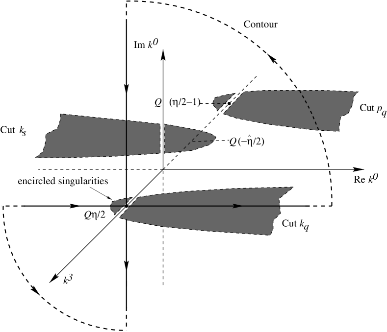
Figure 17: Location of the relevant singularities in the impulse-approximate quark contribution to the form factors. The relative momentum $k$ is the integration variable in the loop diagram corresponding to Eq. (D).

For $Q=0$, i.e., in the rest frame of the nucleon in which the Bethe-Salpeter equation was solved, the naive Wick rotation is justified for $1-\frac{m_{s}}{M}<\eta<\frac{m_{q}}{M}$, since there always is a finite gap between the cuts contained in the hypersurface Re$k^{0}$=0 of the Re$k^{0}$ – Im$k^{0}$ – $\vec{k}$ space. As $Q$ increases, these cuts begin are shifted along both, the $k^{3}$ and the $k^{0}$-axis, as sketched in Figure 17. This eventually amounts to the effect that one of the two cuts arising from each propagator crosses the Im $k^{0}$-axis. As indicated in the figure, Wick rotation $k^{0}\rightarrow ik^{4}$ is no longer possible for arbitrary values of $k^{3}$ without encircling singularities. The corresponding residues thus lead to

$$\langle\widehat{J}^{\mu}_{q}\rangle \rightarrow q_{q}\,\int_{E}\,\frac{d^{4}k}{(2\pi)^{4}}$$

$$\hskip 5.69046pt\widetilde{\bar{\psi}}(-k-\hat{\eta}Q,P^{\prime})\,D(k_{s})S(p_{q})\Gamma^{\mu}_{q}S(k_{q})\widetilde{\psi}(k,P)$$

$$\hskip-25.6073pt+i\int\frac{d^{3}\vec{k}}{(2\pi)^{3}}\;\theta_{\vec{k}}\,\widetilde{\bar{\psi}}(-k^{4}_{pole,1},-\vec{k}-\hat{\eta}\vec{Q},P^{\prime})D(k_{s})S(p_{q})\times$$

$$\hskip-2.84544pt\Gamma^{\mu}_{q}\text{Res}(S(k_{q}))\psi(k^{4}_{pole,1},\vec{k},P)$$

$$+\quad\text{analogous terms for $S(p_{q})$ and $D(k_{s})$}$$

upon transforming Eq. (D) to the Euclidean metric. Here, the residue integral is evaluated at the position of the pole in the incoming quark propagator $S(k_{q})$ on the Euclidean $k^{4}$-axis

$$k_{pole,1}^{4}=-i\eta\sqrt{M^{2}+Q^{2}/4}+iW(m_{q},(\vec{k}-\eta/2\,\vec{Q})^{2})\,,$$

where $\text{Res}(S(k_{q}))$ denotes the corresponding residue, and the abbreviation

$$\theta_{\vec{k}}\equiv\theta\left(\eta\,\omega_{Q}-W(m_{q},(\vec{k}-\eta/2\,\vec{Q})^{2})\right)$$

was adopted to determine the integration domain for which the encircled singularities of Figure 17 contribute.

Analogous integrals over the spatial components of the relative momentum $\vec{k}$ arise from the residues corresponding to the poles in the outgoing quark propagator $S(p_{q})$ and the diquark propagator $D(k_{s})$ as given in Eqs. (D) and (D).

Figure 18: The impulse-approxiamte contribution, corresponding to the diagrams of Fig. 8, to the electric form factor of the proton (employing the dipole diquark amplitude). Results of the BS wave function calculations for the $\eta$-values $1/3$ and $0.4$ are compared to the respective amplitude plus residue calculations. The results are normalized to the latter with $\eta$=1/3.

One verifies that these cuts (as represented by the shaded areas in Fig. 17) never overlap. Pinching of the deformed contour does not occur, since there are no anomalous thresholds for spacelike momentum transfer $Q^{2}$ in these diagrams.

In Figure 18 we compare results for the electric form factor of the proton employing the nucleon BS amplitudes, together with the procedure to account for the singularities as outlined above, with the corresponding wave function calculations. The $n=2$ dipole diquark amplitude of Sec. 3 is employed herein once more. For $\eta=1/3$ the Chebyshev expansion of the BS wave function to 9 orders still turns out insufficient to provide for stable numerical results. This is due to being too close to the range in $\eta$ that requires proper treatment of the diquark pole contribution to the nucleon BSE which, with the present value of
the mass $m_{s}/M=0.7$ is the case for $\eta\leq 1-m_{s}/M=0.3$. The considerably weaker suppression of higher orders in the Chebyshev expansion of the BS wave function as compared to the expansion of the BS amplitude enhances the residual $\eta$-dependence of the observables obtained from the former expansion at a given order, in particular, when it has to reproduce close-by pole contributions in the constituent propagators. The impulse-approximate contributions to $G_{E}$ deviate substantially from those employing the BS amplitude and residue calculations in this case. On the other hand, for values of the momentum partitioning variable which are a little larger than $1/3$ such as $\eta=0.4$ used in the other results of Fig. 18, unique results are obtained from both procedures. Both, the BS wave function and amplitude calculation are in perfect agreement for values of the momentum partitioning that are closer to the middle of the range allowed to $\eta$.

For the seagull and exchange quark contributions corresponding to the diagrams of Fig. 9 an analogous analysis of the singularity structure is considerably more complicated. The explicit inclusion of their contributions which allowed the calculation based on the BS amplitude expansion also of these diagrams is numerically too involved. For these contributions to the form factors we have to resort to the BS wave function calculations. Unlike the impulse-approximate contributions we find, however, that the deviations in the results for the exchange quark and seagull contributions for $\eta=1/3$ and $\eta=0.4$ are smaller than the numerical accuracy of the calculations and thus negligible. We attribute this to the fact that the exchange quark and seagull contributions to the form factors tend to fall off considerably faster with increasing $Q^{2}$ than those of the impulse approximation. This can be seen in Figure 6.2.

Small residual $\eta$-dependences are observed for the momentum transfers above 3GeV² also in the otherwise stable calculations. These give rise to deviations in the results for the form factors of at most 4% which decrease rapidly and become negligible at lower $Q^{2}$.

References

- (1)
- (2) M. Ostrick et. al., Phys. Rev. Lett. 83 (1999), 276.
- (3) I. Passchier et. al., Phys. Rev. Lett. 82 (1999), 4988; D. J. Boersma, for the 9405 Collaboration, e-print, nucl-ex/9908003.
- (4) M. Gell-Mann, Phys. Rev. 8 (1964), 214.
- (5) G. Karl and E. Obryk, Nucl. Phys. B 8 (1968), 609.
- (6) D. Faiman and A. W. Hendry, Phys. Rev. 173 (1968), 1720.
- (7) R. P. Feynman, M. Kislinger and F. Ravndal, Phys. Rev. D 3 (1971), 2706.
- (8) A. Chodos, R. L. Jaffe, K. Johnson, C. Thorn and V. F. Weisskopf, Phys. Rev. D 9 (1974), 3471; A. Chodos, R. L. Jaffe, K. Johnson and C. Thorn, Phys. Rev. D 10 (1974), 2599.
- (9) P. Hasenfratz and J. Kuti, Phys. Rep. 40 (1978), 75.
- (10) T. H. R. Skyrme, Proc. R. Soc. 127 (1961), 260.
- (11) G. S. Adkins, C. R. Nappi and E. Witten, Nucl. Phys. B 228 (1983), 552.
- (12) B. Schwesinger, H. Weigel, G. Holzwarth and A. Hayashi, Phys. Rep. 173 (1989), 173.
- (13) G. Holzwarth (Ed.), Baryons as Skyrme Solitons, World Scientific, Singapore, 1993.
- (14) R. Alkofer, H. Reinhardt and H. Weigel, Phys. Rep. 265 (1996), 139.
- (15) C. V. Christov et al, Prog. Part. Nucl. Phys. 37 (1996), 1.
- (16) H. Reinhard, Phys. Lett. B 244 (1990), 316.
- (17) A. Buck, R. Alkofer, and H. Reinhardt, Phys. Lett. B 286 (1992), 29.
- (18) N. Ishii, W. Bentz and K. Yazaki, Phys. Lett. B301 (1993), 165; Phys. Lett. B 318 (1993), 26; Nucl. Phys. A 587 (1995), 617.
- (19) S. Huang and J. Tjon, Phys. Rev. C 49 (1994), 1702.
- (20) A. Buck, and H. Reinhardt, Phys. Lett. B 356 (1995), 168.
- (21) H. Asami, N. Ishii, W. Bentz and K. Yazaki, Phys. Rev. C 51 (1995), 3388.
- (22) R. T. Cahill Aust. J. Phys. 42 (1989), 171.
- (23) C. J. Burden, R. T. Cahill and J. Praschifka, Aust. J. Phys. 42 (1989), 147.
- (24) A. Chodos and C. Thorn, Phys. Rev. D 12 (1975), 2733.
- (25) M. Rho, Phys. Rep. 240 (1994), 1.
- (26) U. Zückert, R. Alkofer, H. Weigel and H. Reinhardt, Phys. Rev. C 55 (1997), 2030; see also, U. Zückert, Baryonen als Hybride: Chirale Solitonen und gebundene Dreiquarkzustände, Dissertation, Tübingen University, 1996.
- (27) L. von Smekal, A. Hauck, and R. Alkofer, Phys. Rev. Lett. 79 (1997), 3591.
- (28) L. von Smekal, A. Hauck, and R. Alkofer, Ann. Phys. 267 (1998), 1.
- (29) J. Collinge, Variant Creutzfeldt-Jakob disease, The Lancet, 354 (1999), 317.
- (30) C. J. Burden, C. D. Roberts and M. J. Thomson, Phys. Lett. B 371, 163.
- (31) C. D. Roberts, Nucl. Phys. A 605 (1996), 475.
- (32) M. A. Pichowsky and T.-S.H. Lee, Phys. Rev. D 56 (1997), 1644.
- (33) V. A. Miransky, “Dynamical Symmetry Breaking in Quantum Field Theories”, World Scientific, 1993, and references therein.
- (34) C. D. Roberts and A. G. Williams, Prog. Part. Nucl. Phys. 33 (1994), 477.
- (35) P. C. Tandy, Prog. Part. Nucl. Phys. 39 (1997), 117.
- (36) K. Kusaka, G. Piller, A. W. Thomas, and A. G. Williams, Phys. Rev. D 55 (1997), 5299.
- (37) G. Hellstern, R. Alkofer, M. Oettel and H. Reinhardt, Nucl. Phys. A 627 (1997), 679.
- (38) M. Oettel, G. Hellstern, R. Alkofer and H. Reinhardt, Phys. Rev. C 58 (1998), 2459.
- (39) J. Praschifka, R. T. Cahill and C. D. Roberts, Int. J. Mod. Phys. A 4 (1989), 4929.
- (40) A. Bender, C. D. Roberts and L. v. Smekal, Phys. Lett. B 380 (1996), 7.
- (41) G. Hellstern, R. Alkofer and H. Reinhardt, Nucl. Phys. A 625 (1997), 697.
- (42) R. Oehme, Int. J. Mod. Phys. A 10 (1995), 1995.
- (43) J. Praschifka, R. T. Cahill and C. D. Roberts, Mod. Phys. Lett. A 3 (1988), 1595.
- (44) S. Mandelstam, Proc. Roy. Soc. 233 A (1955), 248.
- (45) K. Otha, Phys. Rev. C 40 (1989), 1335.
- (46) S. Wang and M. K. Banerjee, Phys. Rev. C 54 (1996), 2883.
- (47) F. Gross and D. O. Riska, Phys. Rev. C 36 (1987), 1928.
- (48) J. Carlson and R. Schiavilla, Rev. Mod. Phys. 70 (1998), 743.
- (49) A.N. Kvinikhidze and B. Blankleider, Phys. Rev. C 60 (1999), 044003; ibid. 044004.
- (50) J. C. R. Bloch et. al., Phys. Rev. C 60 (1999), 062201; and, e-print, nucl-th/9911068.
- (51) N. Ishii, private discussions; see also, The PCAC Relation in the Nucleon Sector in the NJL Model in the BS/Faddeev Approach, talk presented at KEK-Tanashi Int. Symp., Hadrons and Nuclei, Tokyo, Dec. 1998, Nucl. Phys. A, to be published.
- (52) A.N. Kvinikhidze and B. Blankleider, e-print, nucl-th/9912003.
- (53) R. Peierls, The Commutation Laws of Relativistic Quantum Field Theory, Proc. Roy. Soc. A 214 (1952), 143; see also, Sec. I.4 in R. Haag, Local Quantum Physics Springer, 2nd Edition, 1996.
- (54) I. J. R. Aitchison and A. J. G. Hey, Gauge theories in Particle Physics, Adam Hilger, Bristol and Philadelpia (1989), p.194.
- (55) G. Hoehler et al., Nucl. Phys. B 114 (1976), 505.
- (56) P. E. Bosted et al., Phys. Rev. Lett. 68 (1992), 3841.
- (57) S. Platchkov et al., Nucl. Phys. A 510 (1990), 740.
- (58) C. Weiss, A. Buck, R. Alkofer and H. Reinhardt, Phys. Lett. B312 (1993), 6.
- (59) M. Oettel, R. Alkofer and L. von Smekal, to be published.
- (60) F. T. Hawes and M. A. Pichowsky, Phys. Rev. C 59 (1999), 1743.
- (61) W. H. Press et. al., Numerical Recipes, Cambridge University Press, Cambridge, 1994.