MKPH-T-99-22
Pion Electroproduction on the Nucleon and the Generalized GDH Sum Rule

We present predictions for the spin structure functions of the proton and the neutron in the framework of a unitary isobar model for one-pion photo- and electroproduction. Our results are compared with recent experimental data from SLAC. The first moments of the calculated structure functions fulfill the Gerasimov-Drell-Hearn and Burkhardt-Cottingham sum rules within an error of typically 5-10% for the proton. For the neutron target we find much bigger deviations, in particular the sum rule for $I_{1}(0)+I_{2}(0)$ is heavily violated.

1 Introduction

The spin structure of the nucleon in the resonance region is of particular interest to understand the rapid transition from resonance dominated coherent processes to incoherent processes of deep inelastic scattering (DIS) off the constituents. By scattering polarized lepton beams off polarized targets, it has become possible to determine the spin structure functions $g_{1}$ and $g_{2}$. The results of the first experiments at CERN $\!{}^{{\bf?}}$ and SLAC $\!{}^{{\bf?}}$ sparked considerable interest in the community, because the first moment of $g_{1}$, $\Gamma_{1}=\int^{1}_{0}g_{1}(x)dx$, was found to be substantially smaller than expected from the quark model, in particular from the Ellis-Jaffe sum rule $\!{}^{{\bf?}}$.

Here we present the results of the recently developed Unitary Isobar Model (UIM, Ref. $\!{}^{{\bf?}}$) for the spin asymmetries, structure functions and relevant sum rules in the resonance region. This model describes the presently available data for single-pion photo- and electroproduction up to a total $cm$ energy $W_{\rm max}=1.7$ GeV and for $Q^{2}\leq$ 2 (GeV/c)². It is based on effective Lagrangians for Born terms (background) and resonance contributions, and the respective multipoles are constructed in a gauge-invariant and unitary way for each partial wave. The eta production is included in a similar way $\!{}^{{\bf?}}$, while the contribution of more-pion and higher channels is modeled by comparison with the total cross sections and simple phenomenological assumptions.

2 Formalism

The differential cross section for exclusive electroproduction of mesons from polarized targets using polarized electrons, e.g. $\vec{p}(\vec{e},e^{\prime}\pi^{0})p$ can be parametrized in terms of 18 response functions$\!{}^{{\bf?}}$, a total of 36 is possible if in addition also the recoil polarization is observed. Due to the azimuthal symmetry most of them vanish by integration over the angle $\phi$ and only 5 total cross sections remain. The differential cross section for the electron is then given by

$$\frac{d\sigma}{d\Omega\ dE^{\prime}}=\Gamma\sigma(\nu,Q^{2})\,,$$ (1)

$$\sigma=\sigma_{T}+\epsilon\sigma_{L}+P_{y}\sqrt{2\epsilon(1+\epsilon)}\ \sigma_{LT}+hP_{x}\sqrt{2\epsilon(1-\epsilon)}\ \sigma_{LT^{\prime}}+hP_{z}\sqrt{1-\epsilon^{2}}\sigma_{TT^{\prime}}\,,$$ (2)

where $\Gamma$ is the flux of the virtual photon field and the $\sigma_{i},$ $i=L$, $T$, $LT$, $LT^{\prime}$, $TT^{\prime}$, are functions of the $lab$ energy of the virtual photon $\nu$ and the squared four-momentum transferred $Q^{2}$. These response functions can be separated by varying the transverse polarization $\epsilon$ of the virtual photon as well as the polarizations of the electron ($h$) and proton ($P_{z}$ parallel, $P_{x}$ perpendicular to the virtual photon, in the scattering plane and $P_{y}$ perpendicular to the scattering plane). In particular, $\sigma_{T}$ and $\sigma_{TT^{\prime}}$ can be expressed in terms of the total cross sections for excitation of hadronic states with spin projections $3/2$ and $1/2$: $\sigma_{T}=(\sigma_{3/2}+\sigma_{1/2})/2$ and $\sigma_{TT^{\prime}}=(\sigma_{3/2}-\sigma_{1/2})/2.$

In inclusive electron scattering $\vec{e}+\vec{N}\rightarrow X$, only 4 cross sections $\sigma_{T}$, $\sigma_{L}$, $\sigma_{LT^{\prime}}$ and $\sigma_{TT^{\prime}}$ appear, the fifth cross section, $\sigma_{LT}$, vanishes due to unitarity when all open channels are summed up. The individual channels, however, give finite contributions.

The relations between the $\sigma_{i}$ and the quark structure functions $g_{1}$ and $g_{2}$ can be read off the following equations, which define possible generalizations of the Gerasimov-Drell-Hearn (GDH) integral $\!{}^{{\bf?}}$ and the Burkhardt-Cottingham (BC) sum rule $\!{}^{{\bf?}}$,

$$I_{GDH}(Q^{2}) = \frac{2m^{2}}{Q^{2}}\int_{0}^{x_{0}}\left(g_{1}(x,Q^{2})-\gamma^{2}g_{2}(x,Q^{2})\right)\ dx$$ (3)

$$= \frac{m^{2}}{8\pi^{2}\alpha}\int_{\nu_{0}}^{\infty}(1-x)\left(\sigma_{1/2}-\sigma_{3/2}\right)\ \frac{d\nu}{\nu}\$$

$$I_{1}(Q^{2}) = \frac{2m^{2}}{Q^{2}}\int_{0}^{x_{0}}g_{1}(x,Q^{2})\ dx$$ (4)

$$= \frac{m^{2}}{8\pi^{2}\alpha}\int_{\nu_{0}}^{\infty}\frac{1-x}{1+\gamma^{2}}\left(\sigma_{1/2}-\sigma_{3/2}-2\gamma\,\sigma_{LT^{\prime}}\right)\ \frac{d\nu}{\nu}\$$

$$I_{2}(Q^{2}) = \frac{2m^{2}}{Q^{2}}\int_{0}^{x_{0}}g_{2}(x,Q^{2})\ dx$$ (5)

$$= \frac{m^{2}}{8\pi^{2}\alpha}\int_{\nu_{0}}^{\infty}\frac{1-x}{1+\gamma^{2}}\left(\sigma_{3/2}-\sigma_{1/2}-\frac{2}{\gamma}\,\sigma_{LT^{\prime}}\right)\ \frac{d\nu}{\nu}\ ,$$

$$I_{3}(Q^{2}) = \frac{2m^{2}}{Q^{2}}\int_{0}^{x_{0}}(g_{1}(x,Q^{2})+g_{2}(x,Q^{2}))\ dx$$ (6)

$$= -\frac{m^{2}}{4\pi^{2}\alpha}\int_{\nu_{0}}^{\infty}\frac{1-x}{Q}\,\sigma_{LT^{\prime}}\ d\nu\ =I_{1}+I_{2},$$

where $\gamma=Q/\nu$ and $x=Q^{2}/2m\nu$ the Bjorken scaling variable, with $x_{0}$ ($\nu_{0}$) referring to the inelastic threshold of one-pion production. Since $\sigma_{LT^{\prime}}={\cal O}(Q)$, the real photon limit of the integral $I_{1}$ is given by the GDH sum rule $I_{1}(0)=I_{GDH}(0)=-\kappa_{N}^{2}/4,$ with $\kappa_{N}$ the anomalous magnetic moment of the nucleon. At large $Q^{2}$ the structure functions should depend only on $x,$ i.e. $I_{1}\rightarrow 2m\Gamma_{1}/Q^{2}$ with $\Gamma_{1}=\int g_{1}(x){\rm d}x=$const. In the case of the proton, all experiments for $Q^{2}>1$GeV² yield $\Gamma_{1}>0.$ Therefore, a strong variation of $I_{1}(Q^{2})$ with a zero-crossing at $Q^{2}<1$ GeV² is required in order to reconcile the GDH sum rule with the measurements in the DIS region. The third integral of Eq. (5) is constrained by the BC sum rule, which requires that the inelastic contribution for $0<x<x_{0}$ equals the negative value of the elastic contribution, i.e.

$$I_{2}(Q^{2})=\frac{2m^{2}}{Q^{2}}\int_{0}^{x_{0}}g_{2}(x,Q^{2})\ dx=\frac{1}{4}\frac{G_{M}(Q^{2})-G_{E}(Q^{2})}{1+Q^{2}/4m^{2}}\,G_{M}(Q^{2})\,,$$ (7)

where $G_{M}$ and $G_{E}$ are the magnetic and electric Sachs form factors respectively. At large $Q^{2}$ the integral vanishes as $Q^{-10}$, while at the real photon limit $I_{2}(0)=\kappa_{N}^{2}/4+e_{N}\kappa_{N}/4$, the two terms on the right hand side corresponding to the contributions of $\sigma_{TT^{\prime}}$ and $\sigma_{LT^{\prime}}$ respectively. Finally, Eq. (6) defines an integral $I_{3}(Q^{2})$ as the sum of $I_{1}(Q^{2})$ and $I_{2}(Q^{2})$ and is given by the unweighted integral over the longitudinal transverse interference cross section $\sigma_{LT^{\prime}}$. At the real photon point this integral is given by the GDH and BC sum rules, $I_{3}(0)=e_{N}\kappa_{N}/4$. In particular this vanishes for the neutron target.

3 Unitary Isobar Model

Our calculation for the response functions $\sigma_{i}$ is based on the Unitary Isobar Model (UIM) for one-pion photo- and electroproduction of Ref. $\!{}^{{\bf?}}$. The model is constructed with effective phenomenological Lagrangians for Born terms, vector meson exchange in the $t$ channel (background), and the dominant resonances up to the third resonance region. For each partial wave the multipoles satisfy gauge invariance and unitarity. As in any realistic model a special effort is needed to describe the $s$-channel multipoles $S_{11}$ and $S_{31}$. Even close at threshold these multipoles pick up sizeable imaginary parts that cannot be explained by nucleon resonances. In fact the $S_{11}(1535)$, $S_{11}(1650)$ and the $S_{31}(1620)$ play only a minor role for the complex phase of the $E_{0+}$ multipoles even at higher energies. The main effect arises from pion rescattering. This we can take into account by $K$-matrix unitarization. Furthermore we introduce a mixing of pseudoscalar (PS) and pseudovector (PV) $\pi NN$ coupling in the form

$${\cal L}_{\pi NN}^{HM}=\frac{\Lambda_{m}^{2}}{\Lambda_{m}^{2}+q_{0}^{2}}{\cal L}_{\pi NN}^{PV}+\frac{q_{0}^{2}}{\Lambda_{m}^{2}+q_{0}^{2}}{\cal L}_{\pi NN}^{PS}\,,$$ (8)

where $q_{0}$ is the asymptotic pion momentum in the $\pi N$ $cm$ frame which depends only on $W$ and is not an operator acting on the pion field. From the analysis of the $M_{1-}^{(3/2)}$ and $E_{0+}^{(3/2)}$ multipoles we have found that the most appropriate value for the mixing parameter is $\Lambda_{m}=450$ MeV. This form satisfies gauge invariance and chiral symmetry in the low-energy limit and generates in a simple phenomenological way the effects of pion loops. Expressed in the invariant electroproduction amplitudes $A_{1-6}(s,t,u)$ we find a change from the usual amplitudes for PV coupling only in $A_{1}$,

$$A_{1}^{I}=A_{1}^{I,PV}-\frac{eg}{2m^{2}}F(q_{0}^{2})(\kappa_{V}\delta_{I,+}+\kappa_{S}\delta_{I,0}),$$ (9)

where $I$ denotes the isospin component $(+,-,0)$, $\kappa_{V,S}$ are the isovector and isoscalar anomalous magnetic moments of the nucleon and $F(q_{0}^{2})=q_{0}^{2}/(\Lambda_{m}^{2}+q_{0}^{2})$ is a form factor that vanishes in the chiral limit. Since the modification acts as a contact term and because of the smallness of $\kappa_{S}=-0.06$, only the multipoles $E_{0+}^{(+)}$, $M_{1-}^{(+)}$, $L_{0+}^{(+)}$ and $L_{1-}^{(+)}$ are really affected.

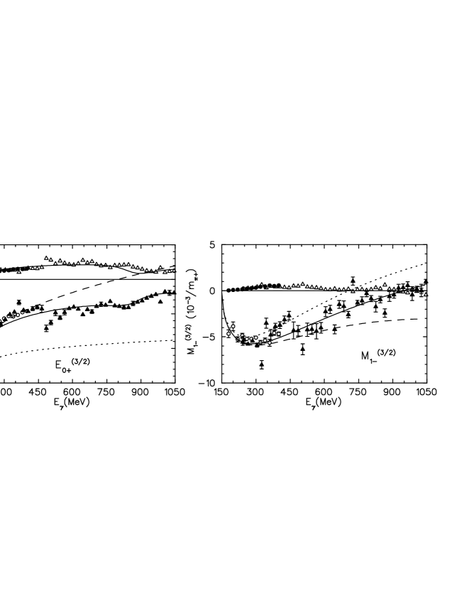
Figure 1: Non-resonant $E_{0+}$ and $M_{1-}$ multipoles calculated with pure pseudovector (dashed curves) and pure pseudoscalar (dotted curves) $\pi NN$ couplings. The solid curves are the results for the real and imaginary parts obtained using the Lagrangian, Eq. (8) and the K-matrix unitarization. The open and full circles are the real and imaginary parts from the Mainz dispersion analysis$\!{}^{{\bf?}}$. The full and open triangles are real and imaginary parts from the VPI analysis$\!{}^{{\bf?}}$.

In Fig. 1 we show a comparison for the non-resonant multipoles $E_{0+}^{(3/2)}$ and $M_{1-}^{(3/2)}$ with the multipole analysis of Hanstein et al.$\!{}^{{\bf?}}$ and the GWU/VPI group$\!{}^{{\bf?}}$. While the PV Born terms very well describe the multipoles in the threshold region, they fail to reproduce the experimental multipoles at higher energies. Furthermore unitarization does not play a very big role in these non-resonant multipoles, in particular for the $P_{31}$, where the imaginary part is very small. Therefore, these two multipoles can ideally be used to fix the free PS-PV mixing parameter $\Lambda_{m}$. Up to a total $cm$ energy $W_{\rm max}=1.7$ GeV and for $Q^{2}\leq$ 2 (GeV/c)² the UIM is able to describe the single-pion electroproduction channel quite well. However, at higher energies the contributions from other channels become increasingly important. In the structure functions $\sigma_{T}$ and $\sigma_{TT^{\prime}}$ we account for the $\eta$ and the multi-pion production contributions extracting the necessary information from the existing data for the total cross section $\!{}^{{\bf?}}$. In Fig. 2 we show the individual channels for the total cross section at $Q^{2}=0$ and at $Q^{2}=0.5GeV^{2}$.

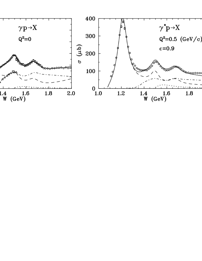
Figure 2: Total cross sections for photoabsorption and inelastic electron scattering on the proton for $\varepsilon=0.9$ and $Q^{2}=0.5\,(GeV/c)^{2}$. Dashed, dotted and dash-dotted curves: contributions of single-pion, eta and multi-pion channels, respectively; solid curves: final result. Experimental data for the total cross sections from Refs.$\!{}^{{\bf?}}$ (x) and $\!{}^{{\bf?}}$ ($\circ$), for the two-pion production channels from Ref.$\!{}^{{\bf?}}$ ($\bigtriangleup$).

Figure 3: The asymmetry $A_{1}+\eta A_{2}$ (top) and the spin structure function $g_{1}$ (bottom) as function of $x$ at $Q^{2}=0.5$ and 1.2 $(GeV/c)^{2}$. Dashed, dotted and solid curves: calculations obtained with $1\pi$, $1\pi+\eta$, and $1\pi+\eta+n\pi$ contributions, respectively. Data from Refs. $\!{}^{{\bf?}}$ ($\bullet$) and $\!{}^{{\bf?}}$ $(\circ)$.

Figure 4: The integrals $I_{GDH}$, $I_{1}$, $I_{2}$ and $I_{3}=I_{1}+I_{2}$ as functions of $Q^{2}$, integrated up to $W_{{\rm max}}=2$ GeV for the proton target. The dashed lines show the contributions from the $1\pi$ channel while the full lines include $1\pi+\eta+n\pi$. The dotted line is the sum rule prediction of Ref. $\!{}^{{\bf?}}$. The data is from Ref.$\!{}^{{\bf?}}$.

Figure 5: The same as Fig. 4 for the neutron target.

In the upper part of Fig. 3, our results for the asymmetry $A_{1}+\eta A_{2}$ are compared with the data from SLAC $\!{}^{{\bf?}}$. The asymmetry is calculated in terms of the virtual photon cross sections by use of the relations $A_{1}=-\sigma_{TT^{\prime}}/\sigma_{T}$ and $A_{2}=-\sigma_{LT^{\prime}}/\sigma_{T}$. We find a reasonable agreement with the data up to $W=2$ GeV. We also note that the contribution of the $\eta$ channel (dotted curves) leads to a substantial increase of the asymmetry over a wide energy region. In the lower part of Fig. 3 we show our results for the structure function $g_{1}.$ Up to a value of $W^{2}=2$ GeV² (corresponding to $x=0.31$ and $x=0.52$ at $Q^{2}$=0.5 and 1.2 (GeV/c)², respectively), the main contribution to $g_{1}$ is due to single-pion production. We clearly note the negative structure above threshold related to excitation of the $\Delta(1232)$ resonance, while in the second and third resonance regions the contributions from $\eta$ and multi-pion channels become increasingly important.

4 Integrals

In Fig. 4 and Fig. 5 we give our predictions for the integrals $I_{GDH}(Q^{2})$, $I_{1}(Q^{2})$, $I_{2}(Q^{2})$ and $I_{3}(Q^{2})$ in the resonance region, i.e. integrated up to $W_{{\rm max}}=2$ GeV for the proton and neutron targets. In the case of the integral $I_{1},$ our model is able to generate the expected drastic change in the helicity structure at low $Q^{2}$. We find a zero-crossing at $Q^{2}=0.75$ (GeV/c)² if we include only the one-pion contribution. This value is lowered to 0.52 (GeV/c)² and 0.45 (GeV/c)² when we include the $\eta$ and the multi-pion contributions respectively. The SLAC analysis yield $I_{1}=0.1\pm 0.06$ at $Q^{2}=0.5$ (GeV/c)², while our result at this point is slightly positive. This deviation could be ascribed mainly to two reasons. First, due to a lack of data points in the $\Delta$ region, the SLAC data are likely to underestimate the $\Delta$ contribution. Second, the strong dependence of the zero-crossing on the multi-pion channels gives rise to uncertainties in our model. A few more data points in the $\Delta$ region would help to clarify this situation. Comparing the two generalizations of the GDH sum rule, $I_{1}(Q^{2})$ and $I_{GDH}(Q^{2})$ it can be seen that the slope at $Q^{2}=0$ depends on the inclusion of the longitudinal contributions. For the proton target the slope gets even an opposite sign with a pronounced minimum for $I_{GDH}$ at $Q^{2}\approx 0.05(GeV/c)^{2}$. This behaviour was also recently obtained in an effective Lagrangian approach $\!{}^{{\bf?}}$.

Concerning the integral $I_{2}$, our full result is in good agreement with the prediction of the BC sum rule. The deviation is within $10~{}\%$ and should be attributed to contributions beyond $W_{\rm max}=2$ GeV and the uncertainties in our calculation for $\sigma_{LT^{\prime}}$. As seen in Eq. (6) the integral $I_{3}$ depends only on this $\sigma_{LT^{\prime}}$ contribution. From the sum rule result a value of $e_{N}\kappa_{N}/4$ is expected at $Q^{2}=0$, i.e. 0.45 for the proton and zero for the neutron target. While our value arising entirely from the $1\pi$ channel gets relatively close to the sum rule result for the proton, in the neutron case this sum rule is heavily violated. So far it is not clear where such a large negative contribution should arise for the neutron target. Either it is due to the high energy tail that may converge rather slowly for the unweighted integral $I_{3}$, or the multi-pion channels could contribute in such a way, while the eta channel is very unlikely. On the other hand the convergence of the BC sum rule cannot be given for granted. In fact Ioffe et al. $\!{}^{{\bf?}}$ have argued that the BC sum rule is valid only in the scaling region, while it is violated by higher twist terms at low $Q^{2}$. In any case a careful study of the multi-pion contribution for both proton and neutron targets will be very helpful, in particular one can expect longitudinal contributions from the non-resonant background.

In Table 1 we list the contributions of the different ingredients of our model to the integrals $I_{1}$, $I_{2}$ and $I_{3}$ at the real photon point, $Q^{2}=0$, for both protons and neutrons. Our values are calculated with the upper limit of integration $W_{\rm max}=2$ GeV. At the photon point the contribution of the $\eta$ and the multi-pion channels tend to cancel each others. This is no longer the case for $Q^{2}\geq 0.4(GeV/c)^{2}$. A complementary analysis to estimate the non-resonance contribution to the generalized GDH integral was recently reported in Ref. $\!{}^{{\bf?}}$.

Table 1: Contributions of the different channels to the integrals $I_{1}$, $I_{2}$ and $I_{3}=I_{1}+I_{2}$ at the photon point, $Q^{2}=0$. (upper part for the proton, lower part for the neutron target)

$I_{1,2,3}$	Born+$\Delta$	$P_{11},D_{13},...$	$\eta$	multi-pion	total	sum rule
$I_{1}$	-0.565	-0.152	0.059	-0.088	-0.746	-0.804
$I_{2}$	1.246	0.063	-0.059	0.088	1.338	1.252
$I_{3}$	0.681	-0.089	0	0	0.592	0.448
$I_{1}$	-0.617	0.061	0.039	-0.064	-0.581	-0.912
$I_{2}$	1.414	-0.075	-0.039	0.064	1.364	0.912
$I_{3}$	0.797	-0.014	0	0	0.783	0

5 Summary

In summary, we have applied our recently developed unitary isobar model for pion electroproduction to calculate generalized GDH integrals and the BC sum rule for both proton and neutron targets. Our results indicate that both the experimental analysis and the theoretical models have to be quite accurate in order to fully describe the helicity structure of the cross section in the resonance region.

While our results agree quite well for the GDH and BC sum rules for the proton, we find substantial deviations for the neutron target, in particular the sum rule $I_{3}(0)\equiv I_{1}(0)+I_{2}(0)=0$ is heavily violated by the contribution from the single-pion channel which is even larger than in the case of the proton.

Concerning the theoretical description, the treatment of the multi-pion channels has to be improved with more refined models. On the experimental side, the upcoming results from measurements with real $\!{}^{{\bf?}}$ and virtual photons $\!{}^{{\bf?}}$ hold the promise to provide new precision data in the resonance region.

References

- [1] EMC Collaboration, J. Ashman et al., Nucl. Phys. B 238, 1 (1989)
- [2] E130 Collaboration, G. Baum et al., Phys. Rev. Lett. 51, 1135 (1983)
- [3] J. Ellis and R. Jaffe, Phys. Rev. D 9, 1444 (1974) and D 10, 1669 (1974).
- [4] D. Drechsel, O. Hanstein, S.S. Kamalov and L. Tiator, Nucl. Phys. A 645, 145 (1999); MAID (an interactive program for pion electroproduction) at www.kph.uni-mainz.de/T/maid/
- [5] G. Knöchlein, D. Drechsel, L. Tiator, Z. Phys. A 352, 327 (1995)
- [6] D. Drechsel and L. Tiator, Journ. Phys. G 18, (1992) 449
- [7] S.B. Gerasimov, Sov. J. Nucl. Phys. 2, 430 (1966); S. D. Drell and A. C. Hearn, Phys. Rev. Lett. 16, 908 (1966)
- [8] H. Burkhardt and W. N. Cottingham, Ann. Phys. (N.Y.) 56, 453 (1970)
- [9] O. Hanstein, D. Drechsel, and L. Tiator, Nucl. Phys. A632 (1998) 561
- [10] R. A. Arndt, I. I. Strakovsky and R. L. Workman, Phys. Rev. C53 (1996) 430 (SP97 solution of the VPI analysis)
- [11] D. Drechsel, S.S. Kamalov, G. Krein, and L. Tiator, Phys. Rev. D 59, 094021 (1999)
- [12] M. MacCormick et al., Phys. Rev. C 53, 41 (1996)
- [13] F. W. Brasse et al., Nucl. Phys. B 110, 413 (1976)
- [14] E143 Collaboration, K. Abe et al., Phys. Rev. D 58, 112003 (1998)
- [15] G. Baum, Phys. Rev. Lett. 45, 2000 (1980)
- [16] O. Scholten and Y.Yu. Korchin, nucl-th/9905004
- [17] B. L. Ioffe, V.A. Khoze, L.N. Lipatov, Hard Processes, North Holland, 1984
- [18] N. Bianchi, and E. Thomas, Phys. Lett. B 450, 439 (1999)
- [19] J. Ahrens et al., MAMI proposal 12/2-93 (1993)
- [20] V. D. Burkert et al., CEBAF PR-91-23 (1991); S. Kuhn et al., CEBAF PR-93-09-(1993; Z. E. Meziani et al., CEBAF PR-94-10-(1994); J. P. Chen et al., TJNAF PR-97-110 (1997)