Deuteron Compton scattering
below pion photoproduction threshold

Abstract

Deuteron Compton scattering below pion photoproduction threshold is considered in the framework of the nonrelativistic diagrammatic approach with the Bonn OBE potential. A complete gauge-invariant set of diagrams is taken into account which includes resonance diagrams without and with $NN$-rescattering and diagrams with one- and two-body seagulls. The seagull operators are analyzed in detail, and their relations with free- and bound-nucleon polarizabilities are discussed. It is found that both dipole and higher-order polarizabilities of the nucleon are required for a quantitative description of recent experimental data. An estimate of the isospin-averaged dipole electromagnetic polarizabilities of the nucleon and the polarizabilities of the neutron is obtained from the data.

PACS: 25.20.Dc, 13.60.Fz

Keywords: Compton scattering; Electromagnetic polarizabilities; Deuteron; Neutron; Meson-exchange currents; Seagulls

I Introduction

Elastic photon, or Compton, scattering is a powerful tool for probing the structure of hadrons and nuclei. A deformation of the system’s ground state caused by an incoming electromagnetic wave and encoded into electromagnetic polarizabilities of the system contributes to radiation of outgoing photons and thus shows itself in such observables as the differential cross section of Compton scattering. A particular example is forward Compton scattering. The corresponding spin-averaged amplitude at sufficiently low energies $\omega$ has the form

$$T(\omega)={\mbox{\boldmath$\bf\epsilon$}}\cdot{\mbox{\boldmath$\bf\epsilon$}}^{\prime*}\Big{(}-\frac{Z^{2}e^{2}}{M_{t}}+4\pi(\bar{\alpha}+\bar{\beta})\omega^{2}+\ldots\Big{)}.$$ (1)

Here $\bf\epsilon$ and ${\mbox{\boldmath$\bf\epsilon$}}^{\prime}$ are polarizations of the initial and final photons, $Ze$ and $M_{t}$ are the electric charge and the mass of the target, and $\bar{\alpha}$ and $\bar{\beta}$ are the electric and magnetic dipole polarizabilities of the target. Many efforts have been spent to measure the polarizabilities of the nucleon, $\bar{\alpha}_{N}$ and $\bar{\beta}_{N}$ (as well as polarizabilities of other hadrons and nuclei), and to understand them theoretically. For a review and further references see [1, 2, 3, 4, 5, 6].

The polarizabilities of the proton have been successfully found in a series of experiments on $\gamma p$ scattering [7, 8, 9, 10, 11, 12, 13] which ultimately yielded quite an accurate result,

$$\bar{\alpha}_{p}=12.1\pm 0.8\pm 0.5,\quad\bar{\beta}_{p}=2.1\mp 0.8\mp 0.5$$ (2)

(in the units of $10^{-4}~{}\rm fm^{3}$ used for the dipole polarizabilities throughout the paper). The values (2) quoted here [12] have been extracted from data of a few experiments of 90’s performed at energies below pion photoproduction threshold under the theoretical constraint of the Baldin sum rule [14, 15]:

$$\bar{\alpha}+\bar{\beta}=\int_{0}^{\infty}\sigma_{\rm tot}(\omega)\,\frac{d\omega}{2\pi^{2}\omega^{2}},$$ (3)

where $\sigma_{\rm tot}(\omega)$ is the total photoabsorption cross section. Recently, the result (2) has been confirmed by a more comprehensive analysis of a larger data base [16].

Meantime, studies of polarizabilities of the neutron which began even earlier than those for the proton (see a book [17] which summarizes a long history of these studies) achieved a knowledge of $\bar{\alpha}_{n}$ and $\bar{\beta}_{n}$ far less satisfactory. Most of the experiments performed for measuring the polarizabilities of the neutron had deals with neutron transmission in the substance. The long-range polarization interaction

$$V_{\rm pol}(r)=-\frac{1}{2}4\pi[\bar{\alpha}{\mbox{\boldmath$\bf E$}}^{2}(r)+\bar{\beta}{\mbox{\boldmath$\bf H$}}^{2}(r)]$$ (4)

of the neutrons with the electromagnetic (actually, electric) field near the edge of nuclei in the substance creates a small but detectable contribution to the total cross section due to its anomalous energy dependence $\propto\sqrt{E}$ [17, 18, 19]. The best results for the electric polarizability of the neutron, $\bar{\alpha}_{n}$, obtained from these studies read [20, 21]

$$\bar{\alpha}_{n}=12.6\pm 1.5\pm 2.0~{}\cite[cite]{[\@@bibref{Number}{schm91}{}{}]},\quad\bar{\alpha}_{n}=0.6\pm 5~{}\cite[cite]{[\@@bibref{Number}{koes95}{}{}]},$$ (5)

where a small relativistic correction $=+0.62$ [3] missing in a fully nonrelativistic formalism used in the original works [18, 20, 21] is included. Since the two values in Eq. (5) seem to contradict to each other, the current situation with knowing the polarizability $\bar{\alpha}_{n}$ is hardly satisfactory. Moreover, there is an argument [23] that the systematic (in fact, theoretical) uncertainty, which is a very delicate problem for those experiments, may be strongly underestimated in Ref. [20]. Furthermore, the neutron transmission experiments do not constrain the magnetic polarizability of the neutron at all, although $\bar{\beta}_{n}$ can be theoretically derived from $\bar{\alpha}_{n}$ by using the Baldin sum rule (3). For all these reasons there is a need for searching for other ways of finding the polarizabilities of the neutron, e.g., by using real photons.

There are several reasons why experimental studies of neutron Compton scattering and a further extraction of the neutron polarizabilities are more difficult than those for the proton. First, because of the absence of dense free-neutron targets, actual measurements of $\gamma n$ scattering are forced to have a deal with neutrons bound in nuclei and hence to take into account effects of the nuclear environment. Second, due to vanishing the neutron Thomson scattering amplitude (viz. the amplitude of photon scattering off the electric charge of the neutron which is zero), the contribution of polarizabilities of the neutron to the differential cross section at low energies ($\lesssim 100$ MeV) turns out to be rather small. It is of order ${\cal O}(\omega^{4})$ in the low-energy expansion over the photon energy $\omega$ vs. order ${\cal O}(\omega^{2})$ in the proton case. Third, the ${\cal O}(\omega^{4})$ contribution of the neutron polarizabilities is accompanied with other terms ${\cal O}(\omega^{4})$ which come from the spin-dependent part of the scattering amplitude; these additional terms are determined by the so-called spin polarizabilities and they cannot be isolated in a model-independent way [24, 25]. Therefore, a use of further assumptions, like those constituting the dispersion theory of Compton scattering [26, 27, 28, 24, 29, 30], for evaluating the unknown pieces becomes unavoidable. All that introduces larger theoretical uncertainties to the obtained polarizabilities which are at least $\pm 2$ even without the nuclear-environment corrections.

The first attempt to measure low-energy $\gamma n$ scattering and to extract polarizabilities of the neutron has been done by the Göttingen–Mainz group [31] which followed an earlier theoretical suggestion [32] to exploit the reaction $\gamma d\to\gamma np$ in the quasi-free kinematics. The result of this very first experiment,

$$\bar{\alpha}_{n}=10.7{\,}^{~{}+3.3}_{-10.7}\,,$$ (6)

is not yet so accurate. However, with the use of a wider range of photon energies (up to 200–250 MeV), further improvements are quite feasible [24, 32, 33]. A high accuracy of the underlying dispersion calculations of $\gamma n$ scattering [24, 29] is crucial for finding the polarizabilities from Compton scattering data taken at “high” energies, viz. those above pion photoproduction threshold. Therefore, a determination of $\bar{\alpha}_{n}$ and $\bar{\beta}_{n}$ from such data also assumes a careful check and normalization of pion photoproduction off the neutron which is used in the dispersion calculations as a crucial input. Fortunately, such a check can be done in parallel with Compton scattering measurements, because the $\gamma(n,\pi)$ reaction can be learned from $\gamma(d,\pi)$ in the quasi-free kinematics as well [34].

In the present work we analyze another possibility for probing the polarizabilities of the neutron which requires no strong assumptions on the “high-energy” behavior of $\gamma N$ interactions. This possibility mentioned already in Ref. [14] is elastic $\gamma d$ scattering below pion photoproduction threshold. The presence of the proton next to the neutron and the coherence of the proton and neutron contributions makes two advantages. First, the ${\cal O}(\omega^{2})$ contribution of the neutron polarizabilities to the scattering amplitude can interfere with the ${\cal O}(1)$ contribution from proton Thomson scattering, so that a sensitivity of the differential cross section with respect to the polarizabilities is enhanced. Second, the largest contribution to the spin polarizabilities of nucleons which comes from the $t$-channel $\pi^{0}$-exchange does not contribute to $\gamma d$ scattering at all (due to isospin), so that ${\cal O}(\omega^{4})$ corrections, which are not small for individual nucleons, especially for the neutron, are more suppressed in the considered case. Nevertheless, various binding corrections, including meson-exchange currents (MEC) and meson-exchange seagulls (MES), are rather important and have to be introduced and carefully evaluated. Their analysis is the central subject of the present paper.

Theoretical studies of deuteron Compton scattering have been started by Bethe and Peierls [35] who considered this process in the dipole $E1$ approximation. After then a number of calculations has been performed in 50’s and 60’s, mostly based on the impulse approximation [36]. A higher level of art, with an explicit consideration of MEC and of their influence on the so-called resonance and seagull amplitudes of Compton scattering was introduced by Weyrauch and Arenhövel [37]. They directly calculated the seagull contribution from the pion exchange and developed an approximate scheme based on dispersion relations in the long wave-length limit to find the resonance amplitude of Compton scattering from a theoretically known deuteron photodisintegration amplitude. Later on, direct calculations of the resonance amplitude free from the approximations of the oversimplified dispersion relations have been performed using a simple separable $NN$ potential [38]. More recently, this consideration was further improved [39] by using realistic $NN$ potentials for evaluation of $NN$ rescattering in the intermediate state and by taking into account leading relativistic corrections and MEC beyond the Siegert approximation. A similar (but technically different) approach was presented by us in Ref.  [40], in which MEC and two-body seagull effects were evaluated using two methods: through a procedure of the minimal substitution in the $NN$ potential and through a direct diagrammatic computation in the framework of the Bonn OBE picture of the $NN$ interactions.

It should be said that despite a resemblance of many physical ingredients of Refs. [37, 38, 39, 40], the results of these works are sometimes rather different, what may indicate unnoticed computational errors or unjustified approximations. For instance, the differential cross section at the forward angle and the photon energy $\omega=100$ MeV found in Ref.  [39] is only 2/3 of that found in Refs. [38, 40] (in this comparison, polarizabilities of the nucleon are omitted). There are large discrepancies at the backward angle either. Very recently, one more calculation in the approach close to that of Ref. [39] was presented [41]. Their results differ from our and previous predictions too, especially at energies $\omega\sim 100$ MeV. Possible reasons for that are discussed in Section VI below.

Recently methods of effective field theories have been applied to deuteron Compton scattering as well [42, 43, 44]. In such an approach, a model-independent part of the low-energy scattering amplitude which dominates in the chiral limit of $m_{\pi}\to 0$ (but still $m_{\pi}^{2}\gg M\Delta$, where $\Delta=2.2246$ MeV is the deuteron binding energy and $M$ is the nucleon mass) was found in a closed analytical form [42]. Generally, the results of both calculations are similar to those obtained by virtue of the “standard-nuclear-theory” technique. The advantage of the calculations [42, 43, 44] is that they naturally include important non-static effects in the pion propagation which is an outside feature for the “standard” theory based on the notion of the $NN$ potential. A disadvantage also exists which is related with unavoidable truncation of the expansion series leading to a lost of contributions important for a determination of the neutron polarizabilities. The $\Delta$-isobar is one example. See Section VI for a further discussion.

In the present paper we complete the calculation with the nonrelativistic Bonn OBE $NN$ potential (OBEPR) started earlier [40]. Technically, this is done in the framework of the diagrammatic approach which relies on an explicit consideration of relevant Feynman diagrams of the reaction in the momentum representation. It avoids Siegert-like transformations and it is rather convenient for incorporating non-static and relativistic corrections [45, 46]. Because of inherent restrictions of the potential picture, our analysis covers energies below pion photoproduction threshold.

Our model is essentially nonrelativistic. However, we include a few most important relativistic corrections (like the spin-orbit interaction) into the one-body electromagnetic current and seagull. After a brief description of the notion of the seagull given in the next Section, we introduce the Hamiltonian of the model and analyze one- and two-body electromagnetic operators. Then we calculate the Compton scattering amplitude and discuss the obtained results.

II Hamiltonians, currents and seagulls

In the framework of the time-ordered perturbation theory, a computation of the photon scattering amplitude starts with a specification of system’s effective degrees of freedom and the system’s Hamiltonian $H[A]$, including its dependence on the external electromagnetic vector potential $A_{\mu}$. We need both linear and quadratic terms in the expansion of $H[A]$ in powers of $A_{\mu}$ which determine operators of the electromagnetic current $j_{\mu}(x)$ and the electromagnetic seagull $S_{\mu\nu}(x,y)$ for the system and, correspondingly, the so-called resonance $R$ and seagull $S$ parts of the Compton scattering amplitude. Simplifying a real situation, we write

$$H[A](t) = H(t)+\int\Big{[}j_{\mu}(x)A^{\mu}(x)\Big{]}_{x_{0}=t}\,d^{3}x$$ (8)

$$\qquad{}-\frac{1}{2}\int\!\!\!\int\Big{[}S_{\mu\nu}(x,y)A^{\mu}(x)A^{\nu}(y)\Big{]}_{x_{0}=y_{0}=t}\,d^{3}x\,d^{3}y+\ldots~{},$$

where $S_{\mu\nu}(x,y)=S_{\nu\mu}(y,x)$ is assumed to be a symmetric function of its arguments. Accordingly, the photon scattering amplitude of

$$|i\rangle+\gamma(\epsilon,k)\to|f\rangle+\gamma^{\prime}(\epsilon^{\prime},k^{\prime})$$ (9)

reads

$$T(\omega,\theta)=R(\omega,\theta)+S(\omega,\theta)$$ (10)

to leading order ${\cal O}(e^{2})$, where

$$R(\omega,\theta)=\sum_{n}\frac{\langle f|\epsilon^{\prime*\mu}j_{\mu}(-k^{\prime})|n\rangle\langle n|\epsilon^{\nu}j_{\nu}(k)|i\rangle}{E_{n}-E_{i}-\omega-i0}+(\epsilon\leftrightarrow\epsilon^{\prime*},k\leftrightarrow-k^{\prime})$$ (11)

and

$$S(\omega,\theta)=\langle f|\epsilon^{\prime*\mu}\epsilon^{\nu}S_{\mu\nu}(-k^{\prime},k)|i\rangle.$$ (12)

Here $\omega=k_{0}$ is the photon energy, $\theta$ is the scattering angle, $E_{n}$ are energies of eigen states $|n\rangle$ of the system, $j_{\mu}(k)$ means a Fourier component of the current density, i.e.

$$j_{\mu}(k)=\int\Big{[}j_{\mu}(x)\,e^{-ik\cdot x}\Big{]}_{x_{0}=0}\,d^{3}x,$$ (13)

and

$$S_{\mu\nu}(-k^{\prime},k)=\int\!\!\!\int\Big{[}S_{\mu\nu}(x,y)\,e^{ik^{\prime}\cdot x-ik\cdot y}\Big{]}_{x_{0}=y_{0}=0}\,d^{3}x\,d^{3}y.$$ (14)

In a more general situation, the Hamiltonian (8) can depend on time derivatives of the vector potential too (e.g. owing to a presence of terms dependent on the electric field). Nothing changes then in Eqs. (11)–(12) with the except that the Fourier components of the current and seagull become dependent on both the space and time components of the photon momenta.

As is well known, the structure of the effective Hamiltonian (and thus that of the current and seagull too) is closely related with a choice of the effective degrees of freedom. In the present context of low-energy deuteron Compton scattering, we consider nonrelativistic nucleons as the only dynamical variables of the system, whereas all mesons, anti-nucleons and other degrees of freedom are encoded into the internal structure and effective interactions of the nucleons themselves. Such an approach is certainly applicable at energies below pion threshold.

With this choice, the resonance amplitude $R$ comes from low-lying (two-nucleon) intermediate excitations $n$ of the deuteron, including the deuteron itself. It corresponds to two-step scattering via photon absorption followed by photon emission and vice versa. This piece can have and generally has the imaginary part. Meanwhile, the seagull amplitude $S$ is real and corresponds to processes, in which the photon absorption and emission happens at indistinguishable time moments, as seen at the considered energy scale. Among such processes are excitations of heavier intermediate states like $\pi NN$, which describe, in particular, meson exchanges between photon interaction points and an internal structure of the nucleon related with intermediate-meson production. Considering meson-exchange processes in general as instantaneous (unretarded) and neglecting dependence of meson propagators on the photon energy, we retain a retardation correction for the pion exchange which is known to be quite important in the seagull amplitude $S$ and to lead to effective modifications of nucleon polarizabilities in nuclei [47]. As for contributions to $S$ due to the nucleon internal structure, it is taken into account by introducing polarizabilities of the nucleon.

Both the current operator $j_{\mu}(x)$ and the seagull operator $S_{\mu\nu}(x,y)$ have to be consistent with the nuclear Hamiltonian $H(t)$ of the system and satisfy conditions of the gauge invariance. Generally, these conditions take the form of the conservation of the electromagnetic current $j_{\mu}[A](x)$ found in the presence of the external vector potential $A_{\mu}$:

$$0=\partial^{\mu}j_{\mu}[A](x)=\partial^{k}j_{k}[A](x)+i\Big{[}H[A](t),j_{0}[A](x)\,\Big{]}+\partial_{A}^{0}j_{0}[A](x).$$ (15)

Here the Latin index $k$ runs over the space components and the time derivative $\partial_{A}^{0}$ acts only on the external potential $A_{\mu}$. In the simplest case of the time-local Hamiltonian (8) the current $j_{\mu}[A](x)$ is given by the three-dimensional variational derivative of $H[A]$,

$$j_{\mu}[A](x)=\frac{\delta H[A](t)}{\delta A^{\mu}(x)}=j_{\mu}(x)-\int S_{\mu\nu}(x,y)A^{\nu}(y)\,d^{3}y+\ldots~{}.$$ (16)

In this case the term with $\partial_{A}^{0}$ in Eq. (15) must vanish, since this is the only piece which depends on the time derivative of $A_{\mu}$. Therefore, the charge density $j_{0}[A](x)$ is $A$-independent, and the following consistency equations emerge [48, 49]:

$$[j_{0}(x),H(t)]=-i\,\frac{\partial j^{k}(x)}{\partial x^{k}}$$ (17)

and

$$[j_{0}(x),j^{\mu}(y)]=i\,\frac{\partial S^{k\mu}(x,y)}{\partial x^{k}},\quad S^{k0}(x,y)=S^{00}(x,y)=0.$$ (18)

Here all operators are taken at the same time moment $t=x_{0}=y_{0}$.

In the nonrelativistic approximation, which will be used in the following consideration of two-body effects, the charge density $j_{0}(x)$ is not affected by meson exchanges (Siegert’s theorem) and therefore coincides with the one-body charge density of the two nucleons $i=1,2$ :

$$j_{0}({\mbox{\boldmath$\bf x$}})=j_{0}^{[1]}({\mbox{\boldmath$\bf x$}})=\sum_{i=1,2}eZ_{i}\delta({\mbox{\boldmath$\bf x$}}-{\mbox{\boldmath$\bf r$}}_{i}),\qquad Z_{i}=\frac{1+\tau_{i}^{z}}{2}.$$ (19)

Then Eqs. (17) and (18) give relations between the nuclear (two-body) potential $V$ standing in the nuclear Hamiltonian $V$ and the two-body parts of the current and seagull, $j_{\mu}^{[2]}$ and $S_{\mu\nu}^{[2]}$ :

$$\Big{[}j_{0}^{[1]}({\mbox{\boldmath$\bf x$}}),V\Big{]}=-i{\mbox{\boldmath$\bf\nabla$}}\cdot{\mbox{\boldmath$\bf j$}}^{[2]}({\mbox{\boldmath$\bf x$}}),$$ (20)

and

$$\Big{[}j_{0}^{[1]}({\mbox{\boldmath$\bf x$}}),j_{l}^{[2]}({\mbox{\boldmath$\bf y$}})\Big{]}=i\,\frac{\partial S_{kl}^{[2]}({\mbox{\boldmath$\bf x$}},{\mbox{\boldmath$\bf y$}})}{\partial x_{k}}.$$ (21)

The resonance and seagull contributions at zero energy are constrained by the Thirring’s low-energy theorem. Within the nonrelativistic accuracy we have

$$T(0,\theta)=R(0,\theta)+S^{[1]}(0,\theta)+S^{[2]}(0,\theta)=-\frac{Z^{2}e^{2}}{AM}\,{\mbox{\boldmath$\bf\epsilon$}}\cdot{\mbox{\boldmath$\bf\epsilon$}}^{\prime*},$$ (22)

where $M$ is the nucleon mass, $Z=1$ and $A=2$ for the deuteron, and the radiation gauge

$$\epsilon_{0}={\mbox{\boldmath$\bf k$}}\cdot{\mbox{\boldmath$\bf\epsilon$}}=0,\quad\epsilon_{0}^{\prime}={\mbox{\boldmath$\bf k$}}^{\prime}\cdot{\mbox{\boldmath$\bf\epsilon$}}^{\prime}=0$$ (23)

is assumed for the photon polarization vectors. In the absence of the two-body currents and seagulls, the model-independent relation (22) is fulfilled due to a balance between the one-body seagull contribution,

$$S^{[1]}(0,\theta)=-\frac{Ze^{2}}{M}\,{\mbox{\boldmath$\bf\epsilon$}}\cdot{\mbox{\boldmath$\bf\epsilon$}}^{\prime*},$$ (24)

and the resonance amplitude $R(0,\theta)=(NZe^{2}/AM){\mbox{\boldmath$\bf\epsilon$}}\cdot{\mbox{\boldmath$\bf\epsilon$}}^{\prime*}$. Here $N=A-Z$. The presence of the two-body currents results in an enhancement of the resonance amplitude, viz. $R(0,\theta)\to(NZe^{2}/AM)(1+\kappa){\mbox{\boldmath$\bf\epsilon$}}\cdot{\mbox{\boldmath$\bf\epsilon$}}^{\prime*}$ for spinless nuclei, where $\kappa$ is the enhancement parameter standing in the modified Thomas-Reiche-Kuhn sum rule (see, e.g., the review [6] for a discussion and further references). Then, in order to support the balance suggested by the low-energy theorem (22), a two-body seagull contribution is required. It is $S^{[2]}(0,\theta)=-(NZe^{2}/AM)\kappa{\mbox{\boldmath$\bf\epsilon$}}\cdot{\mbox{\boldmath$\bf\epsilon$}}^{\prime*}$ for the spinless nucleus. For a general case of a nucleus of spin $S\geq 1$, the two-body seagull amplitude is characterized by the scalar and tensor enhancement parameters, $\kappa$ and $\kappa_{T}$:

$$S^{[2]}(0,\theta)=-\frac{NZ}{AM}e^{2}\epsilon^{\prime*}_{i}\epsilon_{j}\Big{\{}\kappa\delta_{ij}+\kappa_{T}\Big{[}S_{i}S_{j}+S_{j}S_{i}-\frac{2}{3}S(S+1)\delta_{ij}\Big{]}\Big{\}}.$$ (25)

Now we proceed with a consideration of free and interacting nucleons.

III Hamiltonian for a single polarizable nucleon

A Leading-order effects

Phenomenologically, the dipole polarizabilities $\bar{\alpha}$ and $\bar{\beta}$ are defined as low-energy parameters determining the quadratic-in-the-field energy shift $V_{\rm pol}$, Eq. (4). This shift has to be added to a “bare” Hamiltonian $H_{0}[A]$ which is linear in the electromagnetic field, describes an “unpolarizable” nucleon with the electric charge $eZ$ and anomalous magnetic moment $e\kappa/2M$ and produces the so-called Born contribution to the Compton scattering amplitude. In the relativistic phenomenology, the standard choice for $H_{0}[A]$ and hence the standard definition of the unpolarizable nucleon is given by the Dirac–Pauli Hamiltonian

$$H_{0}[A]=eZA_{0}+{\mbox{\boldmath$\bf\alpha$}}\cdot({\mbox{\boldmath$\bf p$}}-eZ{\mbox{\boldmath$\bf A$}})+\beta M+\frac{e\kappa}{4M}\beta\sigma_{\mu\nu}F^{\mu\nu}$$ (26)

with $F_{\mu\nu}=\partial_{\mu}A_{\nu}-\partial_{\nu}A_{\mu}$. Actually, the given form of $H_{0}[A]$ is valid only for the nucleon interacting with real photons. This is all we need in the present paper. In the more general case, additional derivatives of the electromagnetic field appear in $H_{0}[A]$ as well [3]. They account for electromagnetic form factors of the nucleon, i.e. its finite size.

Polarizabilities manifest themselves in low-energy Compton scattering as an ${\cal O}(\omega^{2})$ addition to the Born amplitude, the latter becoming the Thomson scattering amplitude $-(e^{2}Z^{2}/M)\,{\mbox{\boldmath$\bf\epsilon$}}\cdot{\mbox{\boldmath$\bf\epsilon$}}^{\prime*}$ at zero energy. In order to correctly identify the contribution of the polarizabilities, ${\cal O}(\omega^{2})$ terms in the Born amplitude have to be retained as well. Since some of them are of order ${\cal O}(\omega^{2}/M^{3})$, an effective low-energy Hamiltonian covering all the ${\cal O}(\omega^{2})$ terms has to include relativistic corrections up to order ${\cal O}(M^{-3})$.

A nonrelativistic reduction of the Dirac–Pauli Hamiltonian valid to order required was found in Ref. [19]. Using the Foldy–Wouthuysen method [50, 51] or expelling lower components and higher derivatives as described in Refs. [19, 52], a lengthy but straightforward computation gives

$$H_{0}[A] = eZA_{0}+\frac{{\mbox{\boldmath$\bf\pi$}}^{2}}{2M}-\frac{({\mbox{\boldmath$\bf\pi$}}^{2})^{2}}{8M^{3}}-\frac{e(Z+\kappa)}{2M}{\mbox{\boldmath$\bf\sigma$}}\cdot{\mbox{\boldmath$\bf H$}}$$ (31)

$${}-\frac{e(Z+2\kappa)}{8M^{2}}\Big{[}{\mbox{\boldmath$\bf\nabla$}}\cdot{\mbox{\boldmath$\bf E$}}+{\mbox{\boldmath$\bf\sigma$}}\cdot({\mbox{\boldmath$\bf E$}}\times{\mbox{\boldmath$\bf\pi$}}-{\mbox{\boldmath$\bf\pi$}}\times{\mbox{\boldmath$\bf E$}})\Big{]}$$

$${}+\frac{eZ}{8M^{3}}\{{\mbox{\boldmath$\bf\pi$}}^{2},{\mbox{\boldmath$\bf\sigma$}}\cdot{\mbox{\boldmath$\bf H$}}\}+\frac{e\kappa}{8M^{3}}\{{\mbox{\boldmath$\bf\sigma$}}\cdot{\mbox{\boldmath$\bf\pi$}},{\mbox{\boldmath$\bf\pi$}}\cdot{\mbox{\boldmath$\bf H$}}\}$$

$${}+\frac{e\kappa}{16M^{3}}\Big{[}\{{\mbox{\boldmath$\bf\pi$}},{\mbox{\boldmath$\bf\nabla$}}\times{\mbox{\boldmath$\bf H$}}-\dot{{\mbox{\boldmath$\bf E$}}}\}+({\mbox{\boldmath$\bf\sigma$}}\times{\mbox{\boldmath$\bf\nabla$}})\cdot({\mbox{\boldmath$\bf\nabla$}}\times{\mbox{\boldmath$\bf H$}}-\dot{{\mbox{\boldmath$\bf E$}}})\Big{]}$$

$${}+\frac{e^{2}}{8M^{3}}\Big{[}(Z^{2}+Z\kappa+\kappa^{2}){\mbox{\boldmath$\bf E$}}^{2}-Z^{2}{\mbox{\boldmath$\bf H$}}^{2}\Big{]}+{\cal O}(M^{-4}).$$

Here ${\mbox{\boldmath$\bf\pi$}}={\mbox{\boldmath$\bf p$}}-eZ{\mbox{\boldmath$\bf A$}}$ is a covariant momentum, $\{A,B\}$ denotes the symmetrized product $AB+BA$, and $\dot{{\mbox{\boldmath$\bf E$}}}$ means the time derivative of the electric field. In the region lying outside any sources $J_{\mu}$ of the electromagnetic field, the combinations ${\mbox{\boldmath$\bf\nabla$}}\cdot{\mbox{\boldmath$\bf E$}}=J_{0}$ and ${\mbox{\boldmath$\bf\nabla$}}\times{\mbox{\boldmath$\bf H$}}-\dot{{\mbox{\boldmath$\bf E$}}}={\mbox{\boldmath$\bf J$}}$ vanish, so that the above equation turns out even simpler.

When anti-nucleon degrees of freedom are removed and absorbed into new effective interactions, the resulting effective Hamiltonian (31) becomes non-linear in the electromagnetic field. In particular, it contains polarizability-like parts which have to be kept in computations using nonrelativistic variables alone. Among these parts is the term $\kappa^{2}{\mbox{\boldmath$\bf E$}}^{2}$ which imitates a negative electric polarizability of the neutron and which is known due to Foldy [53].

One can easily check that the Hamiltonian (31) exactly reproduces the Born amplitude of nucleon Compton scattering to order ${\cal O}(\omega^{2})$ which is explicitly given, e.g., in Ref. [3]. Moreover, all the ${\cal O}(\omega^{2})$ terms in the scattering amplitude are retained when the kinetic energy in the nucleon propagator is calculated to leading order ${\cal O}(M^{-1})$ (i.e. nonrelativistically), the electromagnetic current is taken to order ${\cal O}(M^{-2})$ (i.e. with the spin-orbit correction), and the full electromagnetic seagull up to order ${\cal O}(M^{-3})$ is taken as it stands in Eq. (31).

In the present work we adopt a few further simplifications to Eq. (31). First, we neglect those parts of the Hamiltonian which do not contribute to the ${\cal O}(\omega^{2})$ terms at all. These are the ${\cal O}(M^{-3})$ parts of the kinetic energy and the current. Second, we neglect the ${\cal O}(M^{-3})$ part of the spin-dependent seagull which gives an ${\cal O}(\omega^{2})$ contribution to the Compton scattering amplitude but does not contribute to the differential cross section of Compton scattering to order ${\cal O}(\omega^{2})$ with unpolarized nucleons. Third, omitting the ${\cal O}(M^{-3})$ component of the kinetic energy, we omit also a $\sim e^{2}Z^{2}/M^{3}$ part of the seagull standing in $-{\mbox{\boldmath$\bf\pi$}}^{4}/8M^{3}$; moreover, we omit such a part in the coefficients of the fields squared. Thus, we use the following effective Hamiltonian for a single nucleon which interacts with real photons:

$$H^{[1]}[A] = eZA_{0}+\frac{{\mbox{\boldmath$\bf\pi$}}^{2}}{2M}-\frac{e(Z+\kappa)}{2M}{\mbox{\boldmath$\bf\sigma$}}\cdot{\mbox{\boldmath$\bf H$}}-\frac{e(Z+2\kappa)}{8M^{2}}{\mbox{\boldmath$\bf\sigma$}}\cdot({\mbox{\boldmath$\bf E$}}\times{\mbox{\boldmath$\bf\pi$}}-{\mbox{\boldmath$\bf\pi$}}\times{\mbox{\boldmath$\bf E$}})$$ (33)

$${}\quad-\frac{1}{2}4\pi(\bar{\alpha}+\delta\alpha_{0}){\mbox{\boldmath$\bf E$}}^{2}-\frac{1}{2}4\pi\bar{\beta}{\mbox{\boldmath$\bf H$}}^{2},$$

where

$$\delta\alpha_{0}=-\frac{e^{2}}{4\pi}\,\frac{\kappa^{2}+Z\kappa}{4M^{3}}=\cases{-0.85,&proton,\cr-0.62,&neutron.}$$ (34)

The corresponding electromagnetic vertices, i.e. matrix elements of the one-body current and seagull in the momentum representation, read

$$\epsilon^{\mu}j_{\mu}^{[1]}(k;p^{\prime},p) = -\frac{eZ}{2M}{\mbox{\boldmath$\bf\epsilon$}}\cdot({\mbox{\boldmath$\bf p$}}+{\mbox{\boldmath$\bf p$}}^{\prime})-\frac{e}{2M}(Z+\kappa)\,i\omega{\mbox{\boldmath$\bf\sigma$}}\cdot{\mbox{\boldmath$\bf s$}}$$ (36)

$$\qquad{}-\frac{e}{8M^{2}}(Z+2\kappa)\,i\omega{\mbox{\boldmath$\bf\sigma$}}\cdot{\mbox{\boldmath$\bf\epsilon$}}\times({\mbox{\boldmath$\bf p$}}+{\mbox{\boldmath$\bf p$}}^{\prime})$$

and

$$\epsilon^{\prime*\mu}\epsilon^{\nu}S_{\mu\nu}^{[1]}(-k^{\prime},k) = -\frac{e^{2}Z^{2}}{M}\,{\mbox{\boldmath$\bf\epsilon$}}\cdot{\mbox{\boldmath$\bf\epsilon$}}^{\prime*}+\frac{e^{2}Z}{4M^{2}}(Z+2\kappa)(\omega+\omega^{\prime})\,i{\mbox{\boldmath$\bf\sigma$}}\cdot{\mbox{\boldmath$\bf\epsilon$}}^{\prime*}\times{\mbox{\boldmath$\bf\epsilon$}}$$ (38)

$$\qquad{}+4\pi\omega\omega^{\prime}(\bar{\alpha}+\delta\alpha_{0})\,{\mbox{\boldmath$\bf\epsilon$}}\cdot{\mbox{\boldmath$\bf\epsilon$}}^{\prime*}+4\pi\omega\omega^{\prime}\bar{\beta}\,{\mbox{\boldmath$\bf s$}}\cdot{\mbox{\boldmath$\bf s$}}^{\prime*},$$

where $\omega$ and $\omega^{\prime}$ are the initial and final photon energies,

$${\mbox{\boldmath$\bf s$}}=\hat{{\mbox{\boldmath$\bf k$}}}\times{\mbox{\boldmath$\bf\epsilon$}},\quad{\mbox{\boldmath$\bf s$}}^{\prime}=\hat{{\mbox{\boldmath$\bf k$}}}^{\prime}\times{\mbox{\boldmath$\bf\epsilon$}}^{\prime}$$ (39)

are the magnetic field vectors, and we have used the radiation gauge (23) for the photon polarization vectors. It is worth mentioning that the absence of the kinetic term $-p^{4}/8M^{3}$ in the Hamiltonian (33) allows us to use self-consistently nonrelativistic phenomenological potentials developed for a description of $NN$ interactions at low energies.

The Hamiltonian (33) with the leading relativistic corrections included possesses an accuracy of about $e^{2}/16\pi M^{3}=0.17\times 10^{-4}~{}\rm fm^{3}$ for treating the leading-order effects of the polarizabilities. For example, being used in the lab frame, the Hamiltonian $H^{[1]}[A]$ and the vertices (36)–(38) generate the following $\gamma N$ scattering amplitude at the forward angle,

$$T_{\rm lab}(\theta=0^{\circ}) = \Big{(}-\frac{e^{2}Z^{2}}{M}+4\pi\omega^{2}(\bar{\alpha}+\bar{\beta})\Big{)}\,{\mbox{\boldmath$\bf\epsilon$}}\cdot{\mbox{\boldmath$\bf\epsilon$}}^{\prime*}$$ (41)

$$\qquad{}-\frac{e^{2}\kappa^{2}}{2M^{2}}\,i\omega{\mbox{\boldmath$\bf\sigma$}}\cdot{\mbox{\boldmath$\bf\epsilon$}}^{\prime*}\times{\mbox{\boldmath$\bf\epsilon$}}+{\cal O}(\omega^{3}).$$

The $\delta\alpha_{0}$ and spin-orbit contributions of the seagull properly correct $\omega$-dependent terms coming from the resonance amplitude $R$ and bring the resulting amplitude (41) into an exact agreement with a known low-energy expansion of $T$ (given, e.g., in Ref. [25]). At the backward angle, the amplitude found with the Hamiltonian (33) reads

$$T_{\rm lab}(\theta=180^{\circ}) = \Big{(}-\frac{e^{2}Z^{2}}{M}+4\pi\omega\omega^{\prime}(\bar{\alpha}-\bar{\beta})\Big{)}\,{\mbox{\boldmath$\bf\epsilon$}}\cdot{\mbox{\boldmath$\bf\epsilon$}}^{\prime*}$$ (43)

$$\qquad{}+\frac{e^{2}(\kappa^{2}+4Z\kappa+2Z^{2})}{4M^{2}}\,i(\omega+\omega^{\prime}){\mbox{\boldmath$\bf\sigma$}}\cdot{\mbox{\boldmath$\bf\epsilon$}}^{\prime*}\times{\mbox{\boldmath$\bf\epsilon$}}+{\cal O}(\omega^{3}).$$

This time an exact result is slightly different. It contains an additional term $(e^{2}Z^{2}/2M^{3})\,\omega\omega^{\prime}{\mbox{\boldmath$\bf\epsilon$}}\cdot{\mbox{\boldmath$\bf\epsilon$}}^{\prime*}$ which comes from a recoil ${\cal O}(\omega^{2})$-correction to the Thomson amplitude and which is lost in Eq. (43) because of omitting the $e^{2}Z^{2}/M^{3}$ pieces of the seagull.

B Polarizabilities and the Baldin sum rule

In the case of $\gamma d$ scattering, the seagull amplitudes (12) for the proton and neutron contribute coherently and dominate the scattering amplitude (10) at energies of a few tens MeV. Their joint result depends only on the isospin-averaged polarizabilities of the nucleon, viz. $\bar{\alpha}_{N}=\frac{1}{2}(\bar{\alpha}_{p}+\bar{\alpha}_{n})$ and $\bar{\beta}_{N}=\frac{1}{2}(\bar{\beta}_{p}+\bar{\beta}_{n})$.

In the following we will consider the difference $\bar{\alpha}_{N}-\bar{\beta}_{N}$ as the only free parameter of the nucleon structure. It is hard to reliably predict this difference, because it can be affected by $t$-channel exchanges with poorly known couplings (like the $\sigma$-meson exchange) – see, e.g., Refs. [1, 3]. Meanwhile the sum $\bar{\alpha}_{N}+\bar{\beta}_{N}$ can be safely found from the well-convergent Baldin sum rule (3). This is quite sufficient in the present context.

There are several evaluations of the dispersion integral in Eq. (3). Earlier calculations gave $\bar{\alpha}_{p}+\bar{\beta}_{p}=14.2\pm(0.3{-}0.5)$ [8, 54, 55, 56] and $\bar{\alpha}_{n}+\bar{\beta}_{n}=15.8\pm 0.5$ [55] (we comment on the other result, $\bar{\alpha}_{n}+\bar{\beta}_{n}=13.3$ [56] below). A recent re-analysis [57] gave lower values:

$$\bar{\alpha}_{p}+\bar{\beta}_{p} = 13.69\pm 0.14,$$ (45)

$$\bar{\alpha}_{n}+\bar{\beta}_{n} = 14.40\pm 0.66.$$ (46)

Doing our own calculations with modern sets of photoabsorption data, we also obtain somewhat lower values than those found in 70’s. However, they are not so low as those in Ref. [57], especially for the neutron.

Specifically, finding $\sigma_{\rm tot}(\omega)$ through the set of pion photoproduction amplitudes of Ref. [58] at energies below 400 MeV, taking total photoabsorption cross sections from Refs. [59, 60] at energies 0.5–1.5 GeV, making a smooth mixture of the “theoretical” [58] and experimental [59, 60] cross sections in between, and using a Regge parameterization of $\sigma_{\rm tot}(\omega)$ at energies $\omega>1.5$ GeV (the same as in Refs. [1, 55]), we obtain

$$\bar{\alpha}_{p}+\bar{\beta}_{p}=14.0,$$ (48)

$$\bar{\alpha}_{n}+\bar{\beta}_{n}=15.2.$$ (49)

Uncertainties in these numbers mainly originate from the region of $\omega\lesssim 500$ MeV which essentially saturates the dispersion integral. They can be again conservatively estimated as $\pm(0.3{-}0.5)$. For example, we obtain very close results (13.8 and 15.2, respectively) using in this computation photo-pion amplitudes from the code SAID [61] (as of beginning of 1999) instead of the amplitudes from Ref. [58]. The lower value for $\bar{\alpha}_{p}+\bar{\beta}_{p}$, which follows from the SAID amplitudes, is mainly caused by that the pion photoproduction multipole $E_{0+}(\pi^{+}n)$, as given by that partial-wave analysis close to pion threshold, is by $\sim 12\%$ too low [62] in comparison with predictions of independent analyses like [58] and with predictions of chiral perturbation theory [63]. In accordance with (III B), we accept the following number for the isospin-averaged sum of the dipole polarizabilities of the nucleon:

$$\bar{\alpha}_{N}+\bar{\beta}_{N}=14.6\,.$$ (50)

There are several reasons why we prefer to rely on our own findings (III B) both for the proton and the neutron rather than on the quoted recent results (III B). For the proton case, the central number for the sum of the polarizabilities obtained by the authors of Ref. [57] is shifted down by their use of the SAID amplitudes very close to pion threshold. This shift almost explains the difference between (45) and (48). It is worth saying that the tiny uncertainty $\pm 0.14$ ascribed to $\bar{\alpha}_{p}+\bar{\beta}_{p}$ in Eq. (45) represents only statistical errors in the experimental data on $\sigma_{\rm tot}$. It does not include systematic errors which are equal to $2{-}3\%$ in $\sigma_{\rm tot}$ and hence produce the uncertainty of at least $\pm 0.3$ in $\bar{\alpha}_{p}+\bar{\beta}_{p}$.

For the neutron, we are even more far from reproducing the very low value obtained in Ref. [57]; we are also far from the result of Ref. [56], where the number obtained was even lower. The reason might be in a different use of the (indirect) data [59] on the neutron total photoabsorption cross section $\sigma_{\rm tot}(\gamma n)$. Close to the $\Delta$-resonance energy, the cross section $\sigma_{\rm tot}(\gamma n)$ given in Ref. [59] is by $\sim 20\%$ (!) lower than predictions of all modern partial-wave analyses of pion photoproduction. The procedure used in Ref. [59] to extract $\sigma_{\rm tot}(\gamma n)$ from the primary cross section $\sigma_{\rm tot}(\gamma d)$ obtained with the deuteron target is not so clear in the $\Delta$-resonance region, in which medium corrections are large. That is why we believe that the results of Ref. [59] for the neutron should not be taken seriously at energies below 400 MeV. As was already said, in our own evaluation of Eq. (49) we have found $\sigma_{\rm tot}(\gamma n)$ below 400 MeV through the partial-wave analyses [58, 61].

C Higher-order corrections

It is clear that higher-order kinematical corrections neglected in Eq. (33) are suppressed by powers of $\omega/M$ and therefore they are small below pion threshold. An actual accuracy of the effective Hamiltonian (33) is determined by dynamical effects which originate from the pion and $\Delta$-isobar structure of the nucleon and give corrections of the relative order $(\omega/m_{\pi})^{2}$. They become important at energies $\gtrsim 70$ MeV. To next-to-leading order, such effects are parametrized by eight structure constants of the nucleon, viz. the quadrupole ($\alpha_{E2}$, $\beta_{M2}$), dispersion ($\alpha_{E\nu}$, $\beta_{M\nu}$) and spin ($\gamma_{E1}$, $\gamma_{M1}$, $\gamma_{E2}$, $\gamma_{M2}$) polarizabilities of the nucleon [64, 65, 66, 25], as represented by the following effective Hamiltonian [25]:

$$\delta H^{[1]}[A] = -\frac{1}{2}4\pi(\alpha_{E\nu}{\mbox{\boldmath$\bf\dot{E}$}}^{2}+\beta_{M\nu}{\mbox{\boldmath$\bf\dot{H}$}}^{2})-\frac{1}{12}4\pi(\alpha_{E2}E_{ij}^{2}+\beta_{M2}H_{ij}^{2})$$ (53)

$${}\qquad-\frac{1}{2}4\pi\Big{(}\gamma_{E1}{\mbox{\boldmath$\bf\sigma$}}\cdot{\mbox{\boldmath$\bf E$}}\times{\mbox{\boldmath$\bf\dot{E}$}}+\gamma_{M1}{\mbox{\boldmath$\bf\sigma$}}\cdot{\mbox{\boldmath$\bf H$}}\times{\mbox{\boldmath$\bf\dot{H}$}}$$

$${}\qquad\qquad-2\gamma_{E2}E_{ij}\sigma_{i}H_{j}+2\gamma_{M2}H_{ij}\sigma_{i}E_{j}\Big{)}.$$

Here

$$E_{ij}=\frac{1}{2}(\nabla_{i}E_{j}+\nabla_{j}E_{i}),\quad H_{ij}=\frac{1}{2}(\nabla_{i}H_{j}+\nabla_{j}H_{i})$$ (54)

are quadrupole strengths of the electric and magnetic fields. Such an effective interaction contributes to the seagull amplitude of $\gamma N$ scattering which gets an addition

$$\epsilon^{\prime*\mu}\epsilon^{\nu}\delta S_{\mu\nu}^{[1]}(-k^{\prime},k)=4\pi\omega\omega^{\prime}\Big{[}{\mbox{\boldmath$\bf\epsilon$}}\cdot{\mbox{\boldmath$\bf\epsilon$}}^{\prime*}\delta\alpha+{\mbox{\boldmath$\bf s$}}\cdot{\mbox{\boldmath$\bf s$}}^{\prime*}\delta\beta$$ (55)

$${}\qquad+\frac{i}{2}(\omega+\omega^{\prime})\Big{(}{\mbox{\boldmath$\bf\sigma$}}\cdot{\mbox{\boldmath$\bf\epsilon$}}^{\prime*}\times{\mbox{\boldmath$\bf\epsilon$}}\,(\gamma_{M2}-\gamma_{E1})+{\mbox{\boldmath$\bf\sigma$}}\cdot{\mbox{\boldmath$\bf s$}}^{\prime*}\times{\mbox{\boldmath$\bf s$}}\,(\gamma_{E2}-\gamma_{M1})\Big{)}$$ (56)

$$\qquad{}-i({\mbox{\boldmath$\bf\sigma$}}\cdot{\mbox{\boldmath$\bf k$}}\,{\mbox{\boldmath$\bf\epsilon$}}\cdot{\mbox{\boldmath$\bf s$}}^{\prime*}-{\mbox{\boldmath$\bf\sigma$}}\cdot{\mbox{\boldmath$\bf k$}}^{\prime}\,{\mbox{\boldmath$\bf s$}}\cdot{\mbox{\boldmath$\bf\epsilon$}}^{\prime*})\gamma_{E2}-i({\mbox{\boldmath$\bf\sigma$}}\cdot{\mbox{\boldmath$\bf k$}}^{\prime}\,{\mbox{\boldmath$\bf\epsilon$}}\cdot{\mbox{\boldmath$\bf s$}}^{\prime*}-{\mbox{\boldmath$\bf\sigma$}}\cdot{\mbox{\boldmath$\bf k$}}\,{\mbox{\boldmath$\bf s$}}\cdot{\mbox{\boldmath$\bf\epsilon$}}^{\prime*})\gamma_{M2}\Big{]}.$$ (57)

The functions $\delta\alpha$, $\delta\beta$ which depend on the photon energies and on the cosine $z=\hat{{\mbox{\boldmath$\bf k$}}}\cdot\hat{{\mbox{\boldmath$\bf k$}}}^{\prime}$ of the scattering angle,

$$\delta\alpha = \omega\omega^{\prime}\Big{(}\alpha_{E\nu}+\frac{z}{6}\alpha_{E2}-\frac{1}{12}\beta_{M2}\Big{)},$$ (58)

$$\delta\beta = \omega\omega^{\prime}\Big{(}\beta_{M\nu}+\frac{z}{6}\beta_{M2}-\frac{1}{12}\alpha_{E2}\Big{)},$$ (59)

can be handled as dynamical corrections to the dipole polarizabilities $\bar{\alpha}$, $\bar{\beta}$ standing in Eq. (38).

Using estimates for the isospin-averaged polarizabilities of the nucleon obtained through fixed-$t$ dispersion relations [25],

$$(\alpha_{E\nu})_{N}\simeq-3.1,\quad(\beta_{M\nu})_{N}\simeq 9.1,\quad(\alpha_{E2})_{N}\simeq 27.3,\quad(\beta_{M2})_{N}\simeq-23.0$$ (60)

(units are $10^{-4}~{}\rm fm^{5}$), we find, e.g., that the contribution of $\delta\alpha$, $\delta\beta$ increases the backward-angle differential cross section of $\gamma d$ scattering and makes the same change as a shift of $\bar{\alpha}_{N}-\bar{\beta}_{N}$ by $-1$, $-2$ and $-4$ at 50 MeV, 70 MeV and 100 MeV, respectively.

It is not easy to estimate a model uncertainty in the above numbers (60). In particular, they are sensitive to the so-called asymptotic contribution $A_{1}^{\rm as}$ to the Compton scattering amplitude $A_{1}$ which was represented by the $\sigma$-exchange of the effective mass $m_{\sigma}=500{-}600$ MeV in the framework of Refs. [25, 29]. Recently, an alternative dispersion approach was presented [30, 67] which allowed to avoid an explicit introduction of the $\sigma$-exchange and to calculate the amplitude $A_{1}$ and the quadrupole polarizabilities of the nucleon under reasonable assumptions on the reactions $\gamma\gamma\to\pi\pi$ and $\pi\pi\to N\bar{N}$. Specific numbers obtained in Ref. [67] for the higher-order polarizabilities (given for the proton case only) are rather close to those obtained earlier [25]. Their use for evaluating the deviation of the backward Compton scattering amplitude from the low-energy expansion of order ${\cal O}(\omega^{2})$, Eq. (43), gives only a 3% bigger effect than that obtained with our numbers (60). More cautiously, we could state that the effect of the quadrupole and dispersion polarizabilities is known within 20%, where the last number is obtained by a reasonable variation of the effective $\sigma$-meson mass.

In order to evaluate the spin-dependent contribution in Eq. (55), we use spin polarizabilities of the nucleon as found through the dispersion relations too [25, 62, 69]:

$$(\gamma_{E1})_{N}\simeq-3.7,\quad(\gamma_{M1})_{N}\simeq 2.3,\quad(\gamma_{E2})_{N}\simeq 1.4,\quad(\gamma_{M2})_{N}\simeq 0.6$$ (61)

(units are $10^{-4}~{}\rm fm^{4}$). Writing Eq. (61), we have corrected predictions for $\gamma$’s of Refs. [25, 62] which include a poorly constrained asymptotic contribution $A_{2}^{\rm as}$ arising in the fixed-$t$ dispersion relation for the invariant amplitude $A_{2}$ of nucleon Compton scattering. Since $A_{2}^{\rm as}$ determines the backward spin polarizability of the nucleon, $\gamma_{\pi}=-\gamma_{E1}+\gamma_{M1}+\gamma_{E2}-\gamma_{M2}$, which was recently re-evaluated through a more reliable backward dispersion relation [69], we have introduced the appropriate changes to $\gamma$’s. Specifically, they are $\delta(\gamma_{E1})_{N}=-\delta(\gamma_{M1})_{N}=-\delta(\gamma_{E2})_{N}=\delta(\gamma_{M2})_{N}=-\frac{1}{4}\delta(\gamma_{\pi})_{N}$, where $\delta(\gamma_{\pi})_{N}\simeq-4$ is a correction to the previous estimate [25, 62] of $(\gamma_{\pi})_{N}$. About one half of that corrections stems from the $\eta$ and $\eta^{\prime}$ exchanges. At backward angles, the spin effects of order ${\cal O}(\omega^{3})$ result in enhancing the coefficient $(e^{2}/4M^{2})(\kappa^{2}+4Z\kappa+2Z^{2})$ in Eq. (43) by $2\pi\omega\omega^{\prime}\gamma_{\pi}$ with $(\gamma_{\pi})_{N}\simeq 7$ and make an increase in the differential cross section of backward-angle $\gamma d$ scattering which is about one third of what the $(\delta\alpha,\delta\beta)$ correction does.

Recently, there was a controversy on the value of $\gamma_{\pi}$, at least for the proton. It was experimentally found [13] that $(\gamma_{\pi})_{p}=-27.1\pm 2.2\,^{+2.8}_{-2.4}$ (in units of $10^{-4}~{}\rm fm^{4}$) and, therefore, it largely deviates from theoretical predictions [25, 62, 69, 70] which give $(\gamma_{\pi})_{p}=-36.7$ to $-39.5$ and $(\gamma_{\pi})_{n}=50.3$ to $52.5$. Taking this deviation seriously and assuming that the isospin-averaged backward spin polarizability $(\gamma_{\pi})_{N}$ may differ from the above-accepted value of $(\gamma_{\pi})_{N}=7$ by as much as $+10$, we should conclude that the theoretical differential cross section of $\gamma d$ scattering at backward angles is visibly enhanced due to the effect of $(\gamma_{\pi})_{N}$. Accordingly, the value of $\bar{\alpha}_{N}-\bar{\beta}_{N}$ extracted, for instance, from 100 MeV data on $\gamma d$ scattering should be shifted up by as much as $+2\times 10^{-4}~{}\rm fm^{3}$, what is not negligible! On the other hand, recent Mainz measurements of backward-angle proton Compton scattering [71] done with the deuterium target give the differential cross section which is lower than that obtained at LEGS [13], and these newer cross sections assume that the theoretical value of $(\gamma_{\pi})_{p}\approx-37$ is fully compatible with the data. Moreover, recent Mainz measurements of proton Compton scattering data done with the hydrogen target [72] seem to fully exclude the previous finding [13] as well and to completely agree with the quoted theoretical predictions. In view of that, we rely our following analysis on the theoretical values of the spin polarizabilities of the nucleon specified by Eq. (61) and assume that the related theoretical uncertainties in extracting $\bar{\alpha}_{N}-\bar{\beta}_{N}$ are less than $\approx 0.5\times 10^{-4}~{}\rm fm^{3}$.

At forward angles, all the higher-order corrections (55) are less important.

IV Two-body currents and seagulls

A Potential-induced electromagnetic currents and seagulls

The remaining part of the Hamiltonian $H[A]$ is related with two-body interactions of the nucleons. In the absence of the electromagnetic fields, such interactions can be represented by a (generally non-local) $NN$-potential $V$ which has to accurately describe differential cross sections and polarization observables in $NN$ scattering at energies below pion threshold, as well as the deuteron binding energy. There are several phenomenological potentials of that sort in the literature. We have chosen to use the Bonn potential (specifically, its nonrelativistic version OBEPR) [73, 74], because it implies a very simple physical picture of one-boson exchanges (OBE) mediating the $NN$ interaction and, in the framework of this picture, allows constructing the meson-exchange current $j_{\mu}^{[2]}$ and the meson-exchange seagull $S_{\mu\nu}^{[2]}$ directly from the corresponding Feynman diagrams. Of course, the OBE picture cannot be true in all detail. However, at least, it takes fully into account the most important long-range contribution, which is the one-pion exchange.

In the momentum representation, the OBEPR potential has the form

$$V({\mbox{\boldmath$\bf p$}}^{\prime}_{1},{\mbox{\boldmath$\bf p$}}^{\prime}_{2};{\mbox{\boldmath$\bf p$}}_{1},{\mbox{\boldmath$\bf p$}}_{2})=\sum_{\alpha=\pi,\eta,\delta,\sigma,\omega,\rho}V^{\alpha}({\mbox{\boldmath$\bf p$}}^{\prime}_{1},{\mbox{\boldmath$\bf p$}}^{\prime}_{2};{\mbox{\boldmath$\bf p$}}_{1},{\mbox{\boldmath$\bf p$}}_{2}),$$ (62)

where ${\mbox{\boldmath$\bf p$}}_{i}$ and ${\mbox{\boldmath$\bf p$}}^{\prime}_{i}$ are the initial and final momenta of the $i$-th nucleon subject to the constraint ${\mbox{\boldmath$\bf p$}}_{1}+{\mbox{\boldmath$\bf p$}}_{2}={\mbox{\boldmath$\bf p$}}^{\prime}_{1}+{\mbox{\boldmath$\bf p$}}^{\prime}_{2}$, and $V^{\alpha}$ are potentials stemming from the exchanges with the specified mesons $\alpha=\pi$, $\eta$, $\delta$ (which is $a_{0}(980)$ in the modern notation), $\sigma$, $\omega$ and $\rho$ (see Fig. 1a).

FIG. 1.: The one-boson-exchange potential (a), and the corresponding meson-exchange current (b) and meson-exchange seagull (c). Strong and radiative $\alpha NN$ vertices include antinucleons (due to PS couplings and/or relativistic corrections) and form factors.

Let us consider in some details the pion exchange which determines the long-range part of $V$ and gives the biggest contribution to the matrix elements of MEC and MES relevant to low-energy $\gamma d$ scattering. The potential $V^{\pi}$ is velocity-independent, i.e. it depends only on the momentum transfer $\bf q$:

$$V^{\pi}({\mbox{\boldmath$\bf q$}})=-\frac{g_{\pi}^{2}}{4M^{2}}\,{\mbox{\boldmath$\bf\sigma$}}_{1}\cdot{\mbox{\boldmath$\bf q$}}\,{\mbox{\boldmath$\bf\sigma$}}_{2}\cdot{\mbox{\boldmath$\bf q$}}\,{\mbox{\boldmath$\bf\tau$}}_{1}\cdot{\mbox{\boldmath$\bf\tau$}}_{2}\,G_{\pi}({\mbox{\boldmath$\bf q$}}).$$ (63)

Here $g_{\pi}$ is the $\pi NN$ coupling constant, and the function $G_{\pi}$,

$$G_{\pi}({\mbox{\boldmath$\bf q$}})=\frac{F_{\pi}^{2}({\mbox{\boldmath$\bf q$}})}{{\mbox{\boldmath$\bf q$}}^{2}+m_{\pi}^{2}},$$ (64)

contains the pion propagator and the $\pi NN$ vertex form factor of the monopole form,

$$F_{\pi}({\mbox{\boldmath$\bf q$}})=\frac{\Lambda_{\pi}^{2}-m_{\pi}^{2}}{\Lambda_{\pi}^{2}+{\mbox{\boldmath$\bf q$}}^{2}},$$ (65)

given by the isospin-averaged mass of the pion, $m_{\pi}$, and the cutoff parameter $\Lambda_{\pi}$.

The pion-exchange current $j_{\mu}^{\pi}$ can be obtained by attaching the photon line to the exchange pion and to the $\pi NN$ vertices as shown in Fig. 1b, in which the electromagnetic $\gamma\pi NN$ vertex arises due to a momentum dependence of the $\pi NN$ coupling. This momentum dependence comes partly from the derivative, or the factor of $\bf q$, standing in the $\pi NN$ vertex (or, equivalently, from a contribution of antinucleons in the formalism of the pseudo-scalar coupling adopted in Refs. [73, 74]). Then the minimal substitution

$${\mbox{\boldmath$\bf\nabla$}}({\mbox{\boldmath$\bf\tau$}}\cdot{\mbox{\boldmath$\bf\pi$}})\to{\mbox{\boldmath$\bf\nabla$}}({\mbox{\boldmath$\bf\tau$}}\cdot{\mbox{\boldmath$\bf\pi$}})-ie{\mbox{\boldmath$\bf A$}}\,\Big{[}\frac{\tau^{z}}{2},{\mbox{\boldmath$\bf\tau$}}\cdot{\mbox{\boldmath$\bf\pi$}}\Big{]}$$ (66)

in the effective $\pi NN$ Lagrangian generates the well-known Kroll–Ruderman component of the $\gamma\pi NN$ vertex. An additional momentum dependence is introduced by the vertex form factor, Eq. (65), and it should also be taken into account.

Without knowing the dynamical nature of $F_{\pi}(q)$, there is no unique way to restore the electromagnetic current associated with the form factor. Different prescriptions proposed in the literature for maintaining gauge invariance in such cases (see, e.g., Refs. [75, 76, 77, 78, 79, 80, 81, 82, 83]) give different answers, especially in the region of high momenta $q$. Fortunately, at low momenta $q\ll\Lambda_{\pi}$ which are only relevant to the present consideration, such ambiguities are expected to be small, as is suggested by the Siegert’s theorem. In the following we choose a simple phenomenological way explicitly formulated by Riska [77] and Mathiot [78]. That is, we assume that the vertex form factor (65) results from a propagation of a fictitious particle $\Lambda$ of the mass $\Lambda_{\pi}$, which has the same quantum numbers as the pion and mediates the pion interaction with the nucleon (see Figs. 2a and 3b). Accordingly, the photon interacts with the particle $\Lambda$ as well (Fig. 2b), and this gives an additional contribution to the vertex $\gamma\pi NN$ which restores the fulfillment of the generalized Ward-Takahashi identities [84] for the transition amplitude of $\gamma N\to\pi N$ and restores the electromagnetic current conservation in the meson-nucleon system.

FIG. 2.: Diagram $a$: the meson-nucleon form factor $F_{\alpha}({\mbox{\boldmath$\bf q$}})$ viewed as resulting from an intermediate heavy-boson exchange $\Lambda$. Diagrams $b$ and $c$: corresponding contributions to the electromagnetic meson-nucleon vertices.

Evaluating the diagrams shown in Fig. 1b with the vertices shown in Fig. 2b and with the static propagators of all particles, we obtain the well-known result for the pion MEC:

$${\mbox{\boldmath$\bf j$}}^{\pi}({\mbox{\boldmath$\bf k$}};{\mbox{\boldmath$\bf p$}}^{\prime}_{1},{\mbox{\boldmath$\bf p$}}^{\prime}_{2};{\mbox{\boldmath$\bf p$}}_{1},{\mbox{\boldmath$\bf p$}}_{2}) = -ie({\mbox{\boldmath$\bf\tau$}}_{1}\times{\mbox{\boldmath$\bf\tau$}}_{2})^{z}\frac{g_{\pi}^{2}}{4M^{2}}\,\Big{[}{\mbox{\boldmath$\bf\sigma$}}_{1}\,({\mbox{\boldmath$\bf\sigma$}}_{2}\cdot{\mbox{\boldmath$\bf q$}}_{2})\,G_{\pi}({\mbox{\boldmath$\bf q$}}_{2})-(1\leftrightarrow 2)\Big{]}$$ (68)

$${}+ie({\mbox{\boldmath$\bf q$}}_{1}-{\mbox{\boldmath$\bf q$}}_{2})\,({\mbox{\boldmath$\bf\tau$}}_{1}\times{\mbox{\boldmath$\bf\tau$}}_{2})^{z}\frac{g_{\pi}^{2}}{4M^{2}}\,{\mbox{\boldmath$\bf\sigma$}}_{1}\cdot{\mbox{\boldmath$\bf q$}}_{1}\,{\mbox{\boldmath$\bf\sigma$}}_{2}\cdot{\mbox{\boldmath$\bf q$}}_{2}\,G_{1\pi}({\mbox{\boldmath$\bf q$}}_{1},{\mbox{\boldmath$\bf q$}}_{2}).$$

Here we introduced the function (cf. Refs. [77, 78, 83])

$$G_{1\pi}({\mbox{\boldmath$\bf q$}}_{1},{\mbox{\boldmath$\bf q$}}_{2})=\frac{F_{\pi}({\mbox{\boldmath$\bf q$}}_{1})\,F_{\pi}({\mbox{\boldmath$\bf q$}}_{2})}{({\mbox{\boldmath$\bf q$}}_{1}^{2}+m_{\pi}^{2})\,({\mbox{\boldmath$\bf q$}}_{2}^{2}+m_{\pi}^{2})}\Bigg{[}1+\frac{{\mbox{\boldmath$\bf q$}}_{1}^{2}+m_{\pi}^{2}}{{\mbox{\boldmath$\bf q$}}_{2}^{2}+\Lambda_{\pi}^{2}}+\frac{{\mbox{\boldmath$\bf q$}}_{2}^{2}+m_{\pi}^{2}}{{\mbox{\boldmath$\bf q$}}_{1}^{2}+\Lambda_{\pi}^{2}}\Bigg{]},$$ (69)

which provides a combination of propagators of the exchanged pion and the particle $\Lambda$ as they appear in the case of a line with one electromagnetic vertex (see Fig. 3b). The vectors

$${\mbox{\boldmath$\bf q$}}_{1}={\mbox{\boldmath$\bf p$}}_{1}^{\prime}-{\mbox{\boldmath$\bf p$}}_{1},\quad{\mbox{\boldmath$\bf q$}}_{2}={\mbox{\boldmath$\bf p$}}_{2}^{\prime}-{\mbox{\boldmath$\bf p$}}_{2}$$ (70)

are the momenta transferred to the nucleons. These momenta are subject to the constraint ${\mbox{\boldmath$\bf q$}}_{1}+{\mbox{\boldmath$\bf q$}}_{2}={\mbox{\boldmath$\bf k$}}$, where $\bf k$ is the momentum of the incoming photon. Using the identity

$$G_{\pi}({\mbox{\boldmath$\bf q$}}_{1})-G_{\pi}({\mbox{\boldmath$\bf q$}}_{2})=({\mbox{\boldmath$\bf q$}}_{2}^{2}-{\mbox{\boldmath$\bf q$}}_{1}^{2})\,G_{1\pi}({\mbox{\boldmath$\bf q$}}_{1},{\mbox{\boldmath$\bf q$}}_{2}),$$ (71)

one can easily check that the pion-exchange current (68) satisfies Eq. (20), which has the following form in the momentum representation:

$${\mbox{\boldmath$\bf k$}}\cdot{\mbox{\boldmath$\bf j$}}^{\pi}({\mbox{\boldmath$\bf k$}};{\mbox{\boldmath$\bf p$}}^{\prime}_{1},{\mbox{\boldmath$\bf p$}}^{\prime}_{2};{\mbox{\boldmath$\bf p$}}_{1},{\mbox{\boldmath$\bf p$}}_{2}) = eV^{\pi}({\mbox{\boldmath$\bf p$}}^{\prime}_{1},{\mbox{\boldmath$\bf p$}}^{\prime}_{2};{\mbox{\boldmath$\bf p$}}_{1}+{\mbox{\boldmath$\bf k$}},{\mbox{\boldmath$\bf p$}}_{2})Z_{1}$$ (73)

$${}-eZ_{1}V^{\pi}({\mbox{\boldmath$\bf p$}}^{\prime}_{1}-{\mbox{\boldmath$\bf k$}},{\mbox{\boldmath$\bf p$}}^{\prime}_{2};{\mbox{\boldmath$\bf p$}}_{1},{\mbox{\boldmath$\bf p$}}_{2})+(1\leftrightarrow 2).$$

Here $Z_{i}$ ($i=1,2$) are the electric charges of the first and second nucleon, Eq. (19).

FIG. 3.: Modifications of a light-boson propagator by intermediate heavy bosons $\Lambda$. Shown are the cases with zero, one, and two photon vertices on the line.

The pion-exchange seagull $S_{\mu\nu}^{\pi}$ is determined by the diagrams shown in Fig. 1c. There, the electromagnetic meson-nucleon vertices include again the form factors generated by the fictitious particle $\Lambda$ through the mechanism shown in Figs. 2b and 2c. In the case of the pion exchange the very first diagram of Fig. 2c is absent. However, it contributes when the strong meson-nucleon vertex of the OBE potential has a quadratic dependence on the particle momenta. This is the case for $\sigma$, $\delta$, $\omega$ and $\rho$ exchanges (see Ref. [74], Appendix A.3). Evaluating the diagrams 1c, we obtain

$$\epsilon_{i}^{\prime*}\epsilon_{j}S_{ij}^{\pi}(-{\mbox{\boldmath$\bf k$}}^{\prime},{\mbox{\boldmath$\bf k$}};{\mbox{\boldmath$\bf p$}}^{\prime}_{1},{\mbox{\boldmath$\bf p$}}^{\prime}_{2};{\mbox{\boldmath$\bf p$}}_{1},{\mbox{\boldmath$\bf p$}}_{2})=\frac{e^{2}g_{\pi}^{2}}{4M^{2}}\,T_{12}\,\Big{[}{\mbox{\boldmath$\bf\sigma$}}_{1}\cdot{\mbox{\boldmath$\bf\epsilon$}}\,{\mbox{\boldmath$\bf\sigma$}}_{2}\cdot{\mbox{\boldmath$\bf\epsilon$}}^{\prime*}\,G_{\pi}({\mbox{\boldmath$\bf K$}}_{1})+(1\leftrightarrow 2)\Big{]}$$ (74)

$$\qquad\qquad{}-\frac{e^{2}g^{2}_{\pi}}{4M^{2}}\,T_{12}\,\Big{\{}\Big{[}{\mbox{\boldmath$\bf\sigma$}}_{1}\cdot{\mbox{\boldmath$\bf\epsilon$}}\,{\mbox{\boldmath$\bf\sigma$}}_{2}\cdot{\mbox{\boldmath$\bf q$}}_{2}\,({\mbox{\boldmath$\bf q$}}_{2}-{\mbox{\boldmath$\bf K$}}_{1})\cdot{\mbox{\boldmath$\bf\epsilon$}}^{\prime*}\,G_{1\pi}({\mbox{\boldmath$\bf K$}}_{1},{\mbox{\boldmath$\bf q$}}_{2})+(1\leftrightarrow 2)\Big{]}$$ (75)

$$\hskip 120.00018pt{}+({\mbox{\boldmath$\bf\epsilon$}}\leftrightarrow{\mbox{\boldmath$\bf\epsilon$}}^{\prime*},~{}{\mbox{\boldmath$\bf K$}}_{1}\leftrightarrow-{\mbox{\boldmath$\bf K$}}_{2})\Big{\}}$$ (76)

$$\qquad\qquad{}+\frac{e^{2}g^{2}_{\pi}}{4M^{2}}\,T_{12}\,{\mbox{\boldmath$\bf\sigma$}}_{1}\cdot{\mbox{\boldmath$\bf q$}}_{1}\,{\mbox{\boldmath$\bf\sigma$}}_{2}\cdot{\mbox{\boldmath$\bf q$}}_{2}\,D_{\pi}({\mbox{\boldmath$\bf q$}}_{1},{\mbox{\boldmath$\bf q$}}_{2},{\mbox{\boldmath$\bf K$}}_{1},{\mbox{\boldmath$\bf K$}}_{2}).$$ (77)

Here ${\mbox{\boldmath$\bf q$}}_{1}$ and ${\mbox{\boldmath$\bf q$}}_{2}$ are again given by Eq. (70), and the vectors ${\mbox{\boldmath$\bf K$}}_{1}$ and ${\mbox{\boldmath$\bf K$}}_{2}$ are defined as

$${\mbox{\boldmath$\bf K$}}_{1} = {\mbox{\boldmath$\bf q$}}_{1}-{\mbox{\boldmath$\bf k$}}=-{\mbox{\boldmath$\bf q$}}_{2}-{\mbox{\boldmath$\bf k$}}^{\prime},$$ (78)

$${\mbox{\boldmath$\bf K$}}_{2} = {\mbox{\boldmath$\bf q$}}_{2}-{\mbox{\boldmath$\bf k$}}=-{\mbox{\boldmath$\bf q$}}_{1}-{\mbox{\boldmath$\bf k$}}^{\prime}.$$ (79)

The isotopic factor $T_{12}$ is equal to

$$T_{12}=T_{21}={\mbox{\boldmath$\bf\tau$}}_{1}\cdot{\mbox{\boldmath$\bf\tau$}}_{2}-\tau_{1}^{z}\tau_{2}^{z}.$$ (80)

The function $D_{\pi}$ is proportional to the amplitude of pion Compton scattering modified by the form factor corrections. It reads

$$D_{\pi}({\mbox{\boldmath$\bf q$}}_{1},{\mbox{\boldmath$\bf q$}}_{2},{\mbox{\boldmath$\bf K$}}_{1},{\mbox{\boldmath$\bf K$}}_{2})=2{\mbox{\boldmath$\bf\epsilon$}}\cdot{\mbox{\boldmath$\bf\epsilon$}}^{\prime*}\,G_{1\pi}({\mbox{\boldmath$\bf q$}}_{1},{\mbox{\boldmath$\bf q$}}_{2})$$ (81)

$$\qquad{}+\Big{[}({\mbox{\boldmath$\bf q$}}_{1}+{\mbox{\boldmath$\bf K$}}_{1})\cdot{\mbox{\boldmath$\bf\epsilon$}}\;({\mbox{\boldmath$\bf q$}}_{2}-{\mbox{\boldmath$\bf K$}}_{1})\cdot{\mbox{\boldmath$\bf\epsilon$}}^{\prime*}\,G_{2\pi}({\mbox{\boldmath$\bf q$}}_{1},{\mbox{\boldmath$\bf q$}}_{2},{\mbox{\boldmath$\bf K$}}_{1})+(1\leftrightarrow 2)\Big{]}.$$ (82)

Here the function

$$G_{2\pi}({\mbox{\boldmath$\bf q$}}_{1},{\mbox{\boldmath$\bf q$}}_{2},{\mbox{\boldmath$\bf K$}})=\frac{F_{\pi}({\mbox{\boldmath$\bf q$}}_{1})\,F_{\pi}({\mbox{\boldmath$\bf q$}}_{2})}{({\mbox{\boldmath$\bf q$}}_{1}^{2}+m_{\pi}^{2})\,({\mbox{\boldmath$\bf q$}}_{2}^{2}+m_{\pi}^{2})\,({\mbox{\boldmath$\bf K$}}^{2}+m_{\pi}^{2})}$$ (83)

$$\qquad{}\times\Bigg{[}\Bigg{(}1+\frac{{\mbox{\boldmath$\bf q$}}_{1}^{2}+m_{\pi}^{2}}{{\mbox{\boldmath$\bf K$}}^{2}+\Lambda_{\pi}^{2}}\Bigg{)}\Bigg{(}1+\frac{{\mbox{\boldmath$\bf q$}}_{2}^{2}+m_{\pi}^{2}}{{\mbox{\boldmath$\bf K$}}^{2}+\Lambda_{\pi}^{2}}\Bigg{)}+\Bigg{(}\frac{{\mbox{\boldmath$\bf q$}}_{1}^{2}+m_{\pi}^{2}}{{\mbox{\boldmath$\bf q$}}_{2}^{2}+\Lambda_{\pi}^{2}}+\frac{{\mbox{\boldmath$\bf q$}}_{2}^{2}+m_{\pi}^{2}}{{\mbox{\boldmath$\bf q$}}_{1}^{2}+\Lambda_{\pi}^{2}}\Bigg{)}\,\frac{{\mbox{\boldmath$\bf K$}}^{2}+m_{\pi}^{2}}{{\mbox{\boldmath$\bf K$}}^{2}+\Lambda_{\pi}^{2}}\Bigg{]}$$ (84)

provides a combination of propagators of the exchanged pion and the particle $\Lambda$ as they appear in the case of a line with two electromagnetic vertices (see Fig. 3c). Writing Eq. (74), we did not assume any special gauge for the photon polarizations. Therefore, that equation specifies all individual components of the tensor $S_{ij}^{\pi}$. Using Eq. (71) and the identity

$$G_{1\pi}({\mbox{\boldmath$\bf q$}}_{1},{\mbox{\boldmath$\bf q$}}_{2})-G_{1\pi}({\mbox{\boldmath$\bf K$}},{\mbox{\boldmath$\bf q$}}_{2})=({\mbox{\boldmath$\bf K$}}^{2}-{\mbox{\boldmath$\bf q$}}_{1}^{2})\,G_{2\pi}({\mbox{\boldmath$\bf q$}}_{1},{\mbox{\boldmath$\bf q$}}_{2},{\mbox{\boldmath$\bf K$}}),$$ (85)

one can check that the obtained MES satisfies Eq. (21). In the momentum representation,

$$-k_{j}S_{ij}^{\pi}(-{\mbox{\boldmath$\bf k$}}^{\prime},{\mbox{\boldmath$\bf k$}};{\mbox{\boldmath$\bf p$}}^{\prime}_{1},{\mbox{\boldmath$\bf p$}}^{\prime}_{2};{\mbox{\boldmath$\bf p$}}_{1},{\mbox{\boldmath$\bf p$}}_{2}) = ej_{i}^{\pi}(-{\mbox{\boldmath$\bf k$}}^{\prime};{\mbox{\boldmath$\bf p$}}^{\prime}_{1},{\mbox{\boldmath$\bf p$}}^{\prime}_{2};{\mbox{\boldmath$\bf p$}}_{1}+{\mbox{\boldmath$\bf k$}},{\mbox{\boldmath$\bf p$}}_{2})Z_{1}$$ (87)

$${}-eZ_{1}j_{i}^{\pi}(-{\mbox{\boldmath$\bf k$}}^{\prime};{\mbox{\boldmath$\bf p$}}^{\prime}_{1}-{\mbox{\boldmath$\bf k$}},{\mbox{\boldmath$\bf p$}}^{\prime}_{2};{\mbox{\boldmath$\bf p$}}_{1},{\mbox{\boldmath$\bf p$}}_{2})+(1\leftrightarrow 2).$$

We may note that formulas for the seagull $S_{ij}^{\pi}$ (in the $\bf r$-space) were derived long ago in Refs. [85, 37] by considering the appropriate Feynman diagrams, and in Ref. [49] by using the minimal substitution. Neither of those considerations, however, takes into account the $\pi NN$ vertex form factor. Therefore, in order to achieve a consistency with the pion-exchange potential (63), we do need Eq. (74).

Meson-exchange currents ${\mbox{\boldmath$\bf j$}}^{\alpha}$ and seagulls $S_{ij}^{\alpha}$ related with other bosons $\alpha$ of the OBE potential can be derived in a similar way. Formulas for ${\mbox{\boldmath$\bf j$}}^{\alpha}$ were already obtained in Ref. [46]. Newer results for $S_{ij}^{\alpha}$ are given in Appendix A.

All the considered MECs and MESs can be called potential-induced, because they contain only those pieces which are intimately related with the OBE potential itself and which are needed to fulfil the electromagnetic current conservation in the $NN$ system as given by Eqs. (15), (20) and (21). Non-potential contributions to ${\mbox{\boldmath$\bf j$}}^{[2]}$ and $S_{ij}^{[2]}$ also exist, and now we proceed with a consideration of them.

B Non-potential contributions

The most important degree of freedom explicitly missing in the OBE-potential picture of the $NN$ interaction at low energies is an excitation of the intermediate $\Delta$-isobar. Nevertheless, within the purely hadron sector (viz. $NN$) effects of the $\Delta$-excitation are indirectly included owing to the use of fitted parameters adjusted to the experimental data on $NN$ scattering. Then, in accordance with the Siegert’s theorem, the electric contributions to MEC and MES found with such parameters take the effects of the $\Delta$ into account as well, at least in the long wave-length approximation.

This mechanism, however, does not work for magnetic contributions to MEC and MES which have to be added independently. The dominating (long-range) parts of such contributions come from the one-pion exchange, and they appear through modifications $\Gamma_{\gamma\pi}^{\Delta}$, $\Gamma_{\gamma\gamma\pi}^{\Delta}$, of the effective $\gamma\pi NN$ and $\gamma\gamma\pi NN$ vertices caused by the $\gamma N\Delta$ transition (see Fig. 4). We do not include similar modifications for the case of the $\rho$ meson, because they are completely negligible in the present context. It is worth noticing that the vertex $\Gamma_{\gamma\gamma\pi}^{\Delta}$ appears due to the momentum dependence of the $\pi N\Delta$ coupling, and it is needed to maintain the gauge-invariance of the resulting Compton scattering amplitude.

FIG. 4.: The effective $\gamma\alpha NN$ and $\gamma\gamma\alpha NN$ vertices. For $\alpha=\pi$ they take into account the $\Delta$-resonance contribution.

Being used for evaluation of the diagrams in Fig. 1b, the $\Gamma_{\gamma\pi}^{\Delta}$ component of the $\gamma\pi NN$ vertex gives the following contribution to MEC:

$${\mbox{\boldmath$\bf j$}}^{\pi\Delta}({\mbox{\boldmath$\bf k$}};{\mbox{\boldmath$\bf p$}}^{\prime}_{1},{\mbox{\boldmath$\bf p$}}^{\prime}_{2};{\mbox{\boldmath$\bf p$}}_{1},{\mbox{\boldmath$\bf p$}}_{2})=\frac{ig_{\pi}g_{\gamma}^{\Delta}g_{\pi}^{\Delta}}{36M^{2}}\Big{[}\frac{{\mbox{\boldmath$\bf\sigma$}}_{2}\cdot{\mbox{\boldmath$\bf q$}}_{2}\,G_{\pi}({\mbox{\boldmath$\bf q$}}_{2})}{M_{\Delta}-M-\omega}\Big{(}2\tau_{2}^{z}-i({\mbox{\boldmath$\bf\tau$}}_{1}\times{\mbox{\boldmath$\bf\tau$}}_{2})^{z}\Big{)}$$ (88)

$$\qquad{}\times(2{\mbox{\boldmath$\bf q$}}_{2}-i{\mbox{\boldmath$\bf\sigma$}}_{1}\times{\mbox{\boldmath$\bf q$}}_{2})\times{\mbox{\boldmath$\bf k$}}+({\mbox{\boldmath$\bf\tau$}}_{1}\to-{\mbox{\boldmath$\bf\tau$}}_{1},~{}{\mbox{\boldmath$\bf\sigma$}}_{1}\to-{\mbox{\boldmath$\bf\sigma$}}_{1},~{}\omega\to-\omega)\Big{]}+(1\leftrightarrow 2).$$ (89)

Writing this equation, we assumed that the form factor of the $\pi N\Delta$ vertex was equal to that of the $\pi NN$ vertex. The mass and couplings of the $\Delta$ are taken to be [86]

$$M_{\Delta}=1225~{}\mbox{MeV},\quad g_{\gamma}^{\Delta}=0.282e\,\frac{M_{\Delta}+M}{m_{\pi}},\quad g_{\pi}^{\Delta}=\frac{2.18}{m_{\pi}}.$$ (90)

Actually, the crossed term in (88), i.e. the term having $M_{\Delta}-M+\omega$ in the denominator, vanishes when the operator ${\mbox{\boldmath$\bf j$}}^{\pi\Delta}$ acts upon the deuteron state which has the isospin $I=0$.

The $\Delta$-isobar contributes to the seagull operator too. This happens in two ways. First, the $\Gamma_{\gamma\pi}^{\Delta}$ component of the $\gamma\pi NN$ vertex works in the diagrams with one or two contact single-photon vertices shown in Fig. 1c. This gives a contribution which, together with pieces without $\Delta$, can be written through (off-shell) pion photoproduction amplitudes as

$$\epsilon^{\prime*}_{i}\epsilon_{j}S_{ij}^{\pi+\pi\Delta}(-{\mbox{\boldmath$\bf k$}}^{\prime},{\mbox{\boldmath$\bf k$}};{\mbox{\boldmath$\bf p$}}^{\prime}_{1},{\mbox{\boldmath$\bf p$}}^{\prime}_{2};{\mbox{\boldmath$\bf p$}}_{1},{\mbox{\boldmath$\bf p$}}_{2})=\frac{T(\gamma N_{1}\to\pi^{a}N^{\prime}_{1})T(\pi^{a}N_{2}\to\gamma^{\prime}N^{\prime}_{2})}{{\mbox{\boldmath$\bf K$}}_{1}^{2}+m_{\pi}^{2}}+(1\leftrightarrow 2),$$ (91)

where ${\mbox{\boldmath$\bf K$}}_{1}$ is given by Eq. (78), and the sum over the pion’s isospin index $a$ is assumed (see Figs. 5a and 6). Second, the $\Gamma_{\gamma\gamma\pi}^{\Delta}$ component of the $\gamma\gamma\pi NN$ vertex works in the first two diagrams of Fig. 1c with the contact two-photon vertex. This gives the contribution shown in Fig. 5b:

$$\epsilon^{\prime*}_{i}\epsilon_{j}S_{ij}^{\pi\Delta(c)}(-{\mbox{\boldmath$\bf k$}}^{\prime},{\mbox{\boldmath$\bf k$}};{\mbox{\boldmath$\bf p$}}^{\prime}_{1},{\mbox{\boldmath$\bf p$}}^{\prime}_{2};{\mbox{\boldmath$\bf p$}}_{1},{\mbox{\boldmath$\bf p$}}_{2})=iT_{12}\frac{g_{\pi}g_{\gamma}^{\Delta}g_{\pi}^{\Delta}}{36M^{2}}\,\Big{\{}\frac{{\mbox{\boldmath$\bf\sigma$}}_{2}\cdot{\mbox{\boldmath$\bf q$}}_{2}\,G_{\pi}({\mbox{\boldmath$\bf q$}}_{2})}{M_{\Delta}-M-\omega}$$ (92)

$$\qquad{}\times\Big{[}2\omega{\mbox{\boldmath$\bf\epsilon$}}^{\prime*}_{\Lambda}\cdot{\mbox{\boldmath$\bf s$}}+2\omega^{\prime}{\mbox{\boldmath$\bf\epsilon$}}_{\Lambda}\cdot{\mbox{\boldmath$\bf s$}}^{\prime*}-i\omega{\mbox{\boldmath$\bf\sigma$}}_{1}\cdot{\mbox{\boldmath$\bf\epsilon$}}^{\prime*}_{\Lambda}\times{\mbox{\boldmath$\bf s$}}+i\omega^{\prime}{\mbox{\boldmath$\bf\sigma$}}_{1}\cdot{\mbox{\boldmath$\bf\epsilon$}}_{\Lambda}\times{\mbox{\boldmath$\bf s$}}^{\prime*}\Big{]}$$ (93)

$$\qquad\qquad\qquad{}+(1\leftrightarrow 2)\Big{\}}+({\mbox{\boldmath$\bf\epsilon$}}\leftrightarrow{\mbox{\boldmath$\bf\epsilon$}}^{\prime*},~{}{\mbox{\boldmath$\bf k$}}\leftrightarrow-{\mbox{\boldmath$\bf k$}}^{\prime},~{}\omega\to-\omega^{\prime}).$$ (94)

Here $\bf s$ and ${\mbox{\boldmath$\bf s$}}^{\prime}$ are given by Eq. (39). The meson-baryon form factor and the appropriate electromagnetic coupling with the fictitious $\Lambda$-boson (Fig. 2b) are included into Eq. (92) via the use of the vertex function $G_{\pi}({\mbox{\boldmath$\bf q$}}_{2})$ and the modified polarization vectors

$${\mbox{\boldmath$\bf\epsilon$}}_{\Lambda}={\mbox{\boldmath$\bf\epsilon$}}-2{\mbox{\boldmath$\bf K$}}_{1}\,\frac{{\mbox{\boldmath$\bf\epsilon$}}\cdot{\mbox{\boldmath$\bf K$}}_{1}}{{\mbox{\boldmath$\bf K$}}_{1}^{2}+\Lambda_{\pi}^{2}}$$ (95)

(and the same for ${\mbox{\boldmath$\bf\epsilon$}}^{\prime}_{\Lambda}$; under the crossing, ${\mbox{\boldmath$\bf K$}}_{1}\to-{\mbox{\boldmath$\bf K$}}_{2}$ and ${\mbox{\boldmath$\bf s$}}\leftrightarrow{\mbox{\boldmath$\bf s$}}^{\prime*}$).

FIG. 5.: The diagrammatic representation of the two-body seagull $S^{[2]}$. The content of the pion photoproduction amplitude $T_{\gamma\pi}$ is explained in Fig. 6.

FIG. 6.: The amplitude of pion photoproduction.

Another feature missing in the potential picture of the $NN$ interaction is that the exchange-boson fields are generally non-static. Non-static, or retardation, effects are most important for the pion exchange due to its large range. It was recently emphasized by Hütt and Milstein in their studies of Compton scattering by heavy nuclei [47] that the retardation correction gives a noticeable contribution to $\pi$-MES and to the Compton scattering amplitude. In the framework of our formalism, we take this correction into account by using the retarded pion propagator in Eq. (91):

$$\frac{1}{{\mbox{\boldmath$\bf K$}}^{2}+m_{\pi}^{2}}\to\frac{1}{{\mbox{\boldmath$\bf K$}}^{2}+m_{\pi}^{2}-\omega^{2}}\simeq\frac{1}{{\mbox{\boldmath$\bf K$}}^{2}+m_{\pi}^{2}}+\frac{\omega^{2}}{({\mbox{\boldmath$\bf K$}}^{2}+m_{\pi}^{2})^{2}}.$$ (96)

Here we neglect the energy carried by the nucleons and replace the pion energy by the photon one, $\omega$. The adopted procedure is not fully self-consistent, because we neglect retardation corrections to the $\pi$-MEC and to the pion-exchange potential $V^{\pi}$. However, the omitted corrections are expected to be less significant than the retardation correction to the seagull amplitude (cf. Refs. [47, 87]).

V Computation of the amplitudes and cross sections

We do actual computations of the scattering amplitude $T(E_{\gamma},\Theta_{\gamma})$ in the center-of-mass frame of the $\gamma d$ system. Accordingly, $\omega=\omega^{\prime}$ and $\bf k$, ${\mbox{\boldmath$\bf k$}}^{\prime}$ mean the energy and momenta of the photons in the CM frame; also, $\Theta_{\gamma}$ means the CM scattering angle. The symbol $E_{\gamma}$ is reserved to denote the photon beam energy in the Lab frame. To specify polarizations of the particles, we introduce the helicities of the photons (viz. $\lambda$ and $\lambda^{\prime}$) and the spin projections of the deuteron and nucleons to the beam direction ${\mbox{\boldmath$\bf e$}}_{z}$ (viz. $m$, $m_{1}$ and $m_{2}$). In the radiation gauge (23),

$${\mbox{\boldmath$\bf\epsilon$}}=-\frac{1}{\sqrt{2}}(\lambda{\mbox{\boldmath$\bf e$}}_{x}+i{\mbox{\boldmath$\bf e$}}_{y}),\quad{\mbox{\boldmath$\bf\epsilon$}}^{\prime}=-\frac{1}{\sqrt{2}}(\lambda^{\prime}{\mbox{\boldmath$\bf e$}}_{x^{\prime}}+i{\mbox{\boldmath$\bf e$}}_{y}),$$ (97)

where the axis $x^{\prime}$ is orthogonal to ${\mbox{\boldmath$\bf k$}}^{\prime}$ and lies in the reaction plane $xz$.

Using the seagull operator $S^{[1]}_{1\,\mu\nu}(-k^{\prime},k)$ specified in Section III, we obtain the one-body seagull amplitude $S^{[1]}(E_{\gamma},\Theta_{\gamma})$ through a loop integral in the momentum space (see Fig. 7a):

$$\langle\lambda^{\prime},m^{\prime}|S^{[1]}(E_{\gamma},\Theta_{\gamma})|\lambda,m\rangle=\int\frac{d{\mbox{\boldmath$\bf p$}}}{(2\pi)^{3}}\Psi_{m_{1}^{\prime}m_{2}}^{m^{\prime}*}\Big{(}{\mbox{\boldmath$\bf p$}}-\frac{1}{2}{\mbox{\boldmath$\bf k$}}^{\prime}\Big{)}\,\Psi_{m_{1}m_{2}}^{m}\Big{(}{\mbox{\boldmath$\bf p$}}-\frac{1}{2}{\mbox{\boldmath$\bf k$}}\Big{)}$$ (98)

$$\qquad\qquad{}\times\langle m_{1}^{\prime},m_{2}|\epsilon^{\prime*}_{i}\epsilon_{j}S^{[1]}_{1\,ij}(-k^{\prime},k)|m_{1},m_{2}\rangle+(1\leftrightarrow 2).$$ (99)

The notation here is that the state-vectors like $|m_{1},m_{2}\rangle$ are used to designate only spin variables of the particles. The momentum variables, if any, are indicated as arguments of the operators. The sum is always taken over spin projections of intermediate nucleons. The subscript 1 in $S^{[1]}_{1\,\mu\nu}(-k^{\prime},k)$ points out that this operator acts on the nucleon 1.

The deuteron wave function $\Psi_{m_{1}m_{2}}^{m}({\mbox{\boldmath$\bf p$}})$ depends on the relative momentum $\bf p$ of the nucleons. For the nonrelativistic Bonn potential, one can use analytical parameterizations of $\Psi_{m_{1}m_{2}}^{m}({\mbox{\boldmath$\bf p$}})$ given in Ref. [46]. Note that the authors of the Bonn potential published three nonrelativistic versions of that potential which we label OBEPR(A), OBEPR(B) and simply OBEPR. The only difference between these versions is in boson’s masses, couplings and form factors used. The parameters of OBEPR are specified in Ref. [73], Table 14. Parameters of OBEPR(A) and OBEPR(B) are given in Ref. [74], Table A.3, part A and part B, respectively. We always give our predictions obtained with the OBEPR version unless other stated explicitly.

Similarly to Eq. (98), the two-body seagull amplitude $S^{[2]}(E_{\gamma},\Theta_{\gamma})$ is given by a two-loop integral over the nucleon’s momenta (see Fig. 7b):

$$\langle\lambda^{\prime},m^{\prime}|S^{[2]}(E_{\gamma},\Theta_{\gamma})|\lambda,m\rangle=\int\!\!\!\int\frac{d{\mbox{\boldmath$\bf p$}}\,d{\mbox{\boldmath$\bf p$}}^{\prime}}{(2\pi)^{6}}\Psi_{m_{1}^{\prime}m_{2}^{\prime}}^{m^{\prime}*}\Big{(}{\mbox{\boldmath$\bf p$}}^{\prime}-\frac{1}{2}{\mbox{\boldmath$\bf k$}}^{\prime}\Big{)}\,\Psi_{m_{1}m_{2}}^{m}\Big{(}{\mbox{\boldmath$\bf p$}}-\frac{1}{2}{\mbox{\boldmath$\bf k$}}\Big{)}$$ (100)

$$\qquad{}\times\langle m_{1}^{\prime},m_{2}^{\prime}|\epsilon^{\prime*}_{i}\epsilon_{j}S^{[2]}_{ij}(-{\mbox{\boldmath$\bf k$}}^{\prime},{\mbox{\boldmath$\bf k$}};{\mbox{\boldmath$\bf p$}}^{\prime}-{\mbox{\boldmath$\bf k$}}^{\prime},-{\mbox{\boldmath$\bf p$}}^{\prime};{\mbox{\boldmath$\bf p$}}-{\mbox{\boldmath$\bf k$}},-{\mbox{\boldmath$\bf p$}})|m_{1},m_{2}\rangle.$$ (101)

To evaluate this amplitude, we perform integrations over $\bf p$, ${\mbox{\boldmath$\bf p$}}^{\prime}$ and sum over spin variables numerically. Some details of the integration procedure are given in Ref. [46].

FIG. 7.: The one- and two-body seagull amplitudes of $\gamma d$ scattering.

In order to calculate the resonance amplitude $R(E_{\gamma},\Theta_{\gamma})$, we introduce the off-shell $T$-matrix of $NN$ scattering, $T_{NN}(E)$, and write the propagator $G(E)=(E-H+i0)^{-1}$ standing in Eq. (11) in the form

$$G(E)=G_{0}(E)+G_{0}(E)\,T_{NN}(E)\,G_{0}(E),$$ (102)

where $G_{0}(E)=(E-H_{0}+i0)^{-1}$ is the propagator of free nucleons. Then $R(E_{\gamma},\Theta_{\gamma})$ turns out to be the sum of two terms, without and with $NN$ rescattering in the intermediate state (see Fig. 8; cf. Ref. [38]). The term without rescattering reads

$$\langle\lambda^{\prime},m^{\prime}|R^{\rm no\,rescat}(E_{\gamma},\Theta_{\gamma})|\lambda,m\rangle=\int\frac{d{\mbox{\boldmath$\bf p$}}}{(2\pi)^{3}}\,\Big{(}\frac{{\mbox{\boldmath$\bf p$}}^{2}}{M}-E_{k}-i0\Big{)}^{-1}$$ (103)

$$\qquad\qquad{}\times\langle\lambda^{\prime},m^{\prime}|T_{\gamma d}(-k^{\prime};{\mbox{\boldmath$\bf p$}};{\mbox{\boldmath$\bf p$}}_{d}+{\mbox{\boldmath$\bf k$}})|m_{1},m_{2}\rangle\,\langle m_{1},m_{2}|T_{\gamma d}(k;{\mbox{\boldmath$\bf p$}};{\mbox{\boldmath$\bf p$}}_{d}+{\mbox{\boldmath$\bf k$}})|\lambda,m\rangle$$ (104)

$$\qquad\qquad\qquad\qquad{}+({\mbox{\boldmath$\bf\epsilon$}}\leftrightarrow{\mbox{\boldmath$\bf\epsilon$}}^{\prime*},~{}k\leftrightarrow-k^{\prime}).$$ (105)

Here $T_{\gamma d}(k;{\mbox{\boldmath$\bf p$}},{\mbox{\boldmath$\bf P$}})$ denotes the amplitude of deuteron photodisintegration without the final-state interaction (see Fig. 9) at the relative momentum $\bf p$ of the intermediate nucleons and the total momentum $\bf P$. The energy $E_{k}$ in Eq. (103) is equal to

$$E_{k}=\omega+\frac{{\mbox{\boldmath$\bf p$}}_{d}^{2}}{4M}-\Delta-\frac{({\mbox{\boldmath$\bf p$}}_{d}+{\mbox{\boldmath$\bf k$}})^{2}}{4M},$$ (106)

where $\Delta$ is the deuteron binding energy. The deuteron momentum ${\mbox{\boldmath$\bf p$}}_{d}$ is equal to $-{\mbox{\boldmath$\bf k$}}$ in the CM frame, and it is unchanged when the crossing transformation $k\leftrightarrow-k^{\prime}$ is applied. The procedure of a computation of $T_{\gamma d}$ was the same as in Ref. [46], and we refer to this paper for further details and comments. Here we note only that the two-body contribution to $T_{\gamma d}$,

$$\langle m_{1},m_{2}|T_{\gamma d}^{[2]}(k;{\mbox{\boldmath$\bf p$}};{\mbox{\boldmath$\bf 0$}})|\lambda,m\rangle=\int\frac{d{\mbox{\boldmath$\bf p$}}^{\prime}}{(2\pi)^{3}}\,\Psi_{m_{1}^{\prime}m_{2}^{\prime}}^{m}\Big{(}{\mbox{\boldmath$\bf p$}}^{\prime}-\frac{1}{2}{\mbox{\boldmath$\bf k$}}\Big{)}$$ (107)

$$\qquad\qquad{}\times\langle m_{1},m_{2}|{\mbox{\boldmath$\bf\epsilon$}}\cdot{\mbox{\boldmath$\bf j$}}^{[2]}({\mbox{\boldmath$\bf k$}};{\mbox{\boldmath$\bf p$}},-{\mbox{\boldmath$\bf p$}};{\mbox{\boldmath$\bf p$}}^{\prime}-{\mbox{\boldmath$\bf k$}},-{\mbox{\boldmath$\bf p$}}^{\prime})|m_{1}^{\prime},m_{2}^{\prime}\rangle,$$ (108)

contains a loop integral over ${\mbox{\boldmath$\bf p$}}^{\prime}$. Since we do not carry out angular integrations analytically, the evaluation of Eq. (103) actually involves a 9-dimensional numerical integration. Such a computational work was hard but it was done with reasonable computer resources. We have carefully controlled that the number of chosen nodes of integrations was sufficient to predict the observables of $\gamma d$ scattering like the differential cross section with the numerical accuracy better than 1%.

FIG. 8.: The resonance contribution $R$. Shown are terms without and with $NN$-rescattering.

FIG. 9.: Structure of the $\gamma d\to NN$ vertex.

The resonance amplitude with $NN$ rescattering has the form

$$\langle\lambda^{\prime},m^{\prime}|R^{\rm rescat}(E_{\gamma},\Theta_{\gamma})|\lambda,m\rangle=-\int\frac{d{\mbox{\boldmath$\bf p$}}\,d{\mbox{\boldmath$\bf p$}}^{\prime}}{(2\pi)^{6}}\Big{(}\frac{{\mbox{\boldmath$\bf p$}}^{2}}{M}-E_{k}-i0\Big{)}^{-1}\Big{(}\frac{{\mbox{\boldmath$\bf p$}}^{\prime 2}}{M}-E_{k}-i0\Big{)}^{-1}$$ (109)

$$\qquad\qquad{}\times\langle\lambda^{\prime},m^{\prime}|T_{\gamma d}(-k^{\prime};{\mbox{\boldmath$\bf p$}}^{\prime};{\mbox{\boldmath$\bf p$}}_{d}+{\mbox{\boldmath$\bf k$}})|m_{1}^{\prime},m_{2}^{\prime}\rangle\,\langle m_{1}^{\prime},m_{2}^{\prime}|T_{NN}(E_{k};{\mbox{\boldmath$\bf p$}}^{\prime},{\mbox{\boldmath$\bf p$}})|m_{1},m_{2}\rangle$$ (110)

$$\qquad\qquad\qquad\qquad{}\times\langle m_{1},m_{2}|T_{\gamma d}(k;{\mbox{\boldmath$\bf p$}};{\mbox{\boldmath$\bf p$}}_{d}+{\mbox{\boldmath$\bf k$}})|\lambda,m\rangle+({\mbox{\boldmath$\bf\epsilon$}}\leftrightarrow{\mbox{\boldmath$\bf\epsilon$}}^{\prime*},~{}k\leftrightarrow-k^{\prime}).$$ (111)

Here the $NN$ scattering $T$-matrix is determined by the $NN$ potential $V$ through the Lippmann-Schwinger equation $T_{NN}(E)=V+VG_{0}(E)\,T_{NN}(E)$. It is difficult to evaluate Eq. (109) straightforwardly. In order to simplify the computation, we used a separable approximation to $T_{NN}$. Actually, we took $T_{NN}$ from Ref. [88], in which the separable $T$-matrix was built for the Paris potential [89] (see Ref. [32] for an explicit form of $T_{NN}$ given in our notation and normalization).

Since the off-shell properties of $T_{NN}$ for the Paris and Bonn potentials are not the same, the use of the “Paris” $T$-matrix in Eq. (109) spoils the self-consistency of the whole calculation and even violates the gauge invariance of the resulting Compton scattering amplitude. A small mismatch appears between the resonance and seagull amplitudes at all energies, so that the balance (22) prescribed by the low-energy theorem is not exactly fulfilled. At zero energy and forward scattering angle we get $T_{\rm s.a.}(0,0)=-0.47$ for the spin-averaged (s.a.) amplitude of deuteron Compton scattering instead of the correct value of $-0.50$ (it is given in units of $e^{2}/M$ used here and below for the amplitude). For the spin-flip (s.f.) $\gamma d\to\gamma d$ transition $|1,-1\rangle\to|{-1},1\rangle$ we get $T_{\rm s.f.}(0,0)=-0.02$ instead of zero.

We believe, however, that the use of the “Paris” $T$-matrix in Eq. (109) does not lead to practical problems at energies of a few tens MeV, because the rescattering contribution decreases with the energy. For example, at $E_{\gamma}=50$ MeV and $\Theta_{\gamma}=0$ the amplitude (109) is equal to $R^{\rm rescat}_{\rm s.a.}=0.009-i0.076$, what should be compared with the rest amplitude $T^{\rm no\,rescat}_{\rm s.a.}=-1.097+i0.315$ (found without nucleon-polarizability corrections). At larger angles the role of the rescattering contribution is even less important, as will be illustrated in the next Section.

Given the Compton scattering amplitude $\langle\lambda^{\prime},m^{\prime}|T|\lambda,m\rangle$, we find the differential cross section of $\gamma d$ scattering in the CM frame as

$$\frac{d\sigma}{d\Omega_{\gamma}}=\frac{1}{6}\left(\frac{E_{d}}{4\pi W}\right)^{2}\sum_{\lambda^{\prime}m^{\prime},\lambda m}|\langle\lambda^{\prime},m^{\prime}|T|\lambda,m\rangle|^{2},$$ (112)

where $E_{d}=\sqrt{(2M-\Delta)^{2}+\omega^{2}}$ and $W=E_{d}+\omega$ are the deuteron and total energies in the CM frame. The photon beam asymmetry is

$$\Sigma=\frac{d\sigma^{\perp}-d\sigma^{\parallel}}{d\sigma^{\perp}+d\sigma^{\parallel}}=\frac{2\,{\rm Re}\,\sum_{\lambda^{\prime}m^{\prime},m}\,\langle\lambda^{\prime},m^{\prime}|T|1,m\rangle\,\langle\lambda^{\prime},m^{\prime}|T|{-1},m\rangle^{*}}{\sum_{\lambda^{\prime}m^{\prime},\lambda m}|\langle\lambda^{\prime},m^{\prime}|T|\lambda,m\rangle|^{2}},$$ (113)

where $d\sigma^{\perp}$ and $d\sigma^{\parallel}$ are the differential cross sections for the incoming photons polarized perpendicular or parallel to the reaction plane $xz$, respectively.

VI Results and discussion

A Zero-range limit

Before discussing results of the full model, let us consider the limiting case of a very weak binding of the deuteron. Specifically, let us assume that the typical nucleon momentum $\alpha=\sqrt{M\Delta}$, which is 45.7 MeV in reality, is much less than the pion mass. Said differently, we assume that the inter-nucleon distance $r\sim\alpha^{-1}$ in the deuteron is much larger than the $NN$-potential range. Moreover, we assume that the photon energy is also small, $\omega={\cal O}(\alpha)$, so that all effects related with recoil corrections $1/M$ can be safely neglected too. In this limit the two-body contributions to the electromagnetic current and seagull become negligible, and so does the rescattering contribution (109). Therefore, the Compton scattering amplitude is determined by the one-loop diagrams involving the operators $S^{[1]}$, ${\mbox{\boldmath$\bf j$}}^{[1]}$ and the asymptotic wave function of the deuteron,

$$\Psi^{m}_{m_{1}m_{2}}({\mbox{\boldmath$\bf p$}})\simeq\frac{\sqrt{8\pi\alpha}}{{\mbox{\boldmath$\bf p$}}^{2}+\alpha^{2}}\,C^{1m}_{\frac{1}{2}m_{1},\frac{1}{2}m_{2}}\,.$$ (114)

Here $C^{1m_{d}}_{\frac{1}{2}m_{1},\frac{1}{2}m_{2}}$ is the Clebsch-Gordon coefficient. Keeping the terms of leading order over $1/M$ in the electromagnetic operators and in the energy (106) of the intermediate nucleons, and calculating analytically the integrals (98) and (103), one arrives at the following $\gamma d$ scattering amplitude [35, 42]:

$$T(E_{\gamma},\Theta_{\gamma})\simeq\frac{e^{2}}{M}{\mbox{\boldmath$\bf\epsilon$}}\cdot{\mbox{\boldmath$\bf\epsilon$}}^{\prime*}\Big{\{}{-}F_{0}(q)-\frac{4}{3w^{2}}+\frac{2}{3w^{2}}\Big{[}(1-w-i0)^{3/2}+(1+w)^{3/2}\Big{]}\Big{\}},$$ (115)

where

$$F_{0}(q)=\frac{4\alpha}{q}\,\arctan\frac{q}{4\alpha}$$ (116)

is the deuteron form factor in the considered zero-range limit, $q=|{\mbox{\boldmath$\bf k$}}-{\mbox{\boldmath$\bf k$}}^{\prime}|$, and $w=E_{\gamma}/\Delta$. The term with $F_{0}(q)$ in Eq. (115) represents the seagull contribution, whereas other pieces come from the resonance amplitude $R(E_{\gamma},\Theta_{\gamma})$.

As a by-product of this computation, the total cross section $\sigma^{\gamma d\to pn}_{\rm tot}(E_{\gamma})$ of deuteron photodisintegration can be derived through the imaginary part of the (spin-averaged) forward scattering amplitude (115):

$$\,{\rm Im}\,T_{\rm s.a.}(E_{\gamma},0)=E_{\gamma}\sigma^{\gamma d\to pn}_{\rm tot}(E_{\gamma})\simeq\frac{2e^{2}}{3Mw^{2}}(w-1)^{3/2}.$$ (117)

When the photon energy becomes much higher than the deuteron binding energy $\Delta$, the amplitude (115) becomes equal to the proton Thomson scattering amplitude times the deuteron form factor $F_{0}(q)$. This is just the seagull contribution $S(E_{\gamma},\Theta_{\gamma})$ to the amplitude (115). The rest ($w$-dependent) terms in Eq. (115) give the resonance amplitude $R(E_{\gamma},\Theta_{\gamma})$ which vanishes in the limit of $E_{\gamma}\gg\Delta$. An instructive feature of Eq. (115) is however that this vanishing is rather slow, like $\propto E_{\gamma}^{-1/2}$. Therefore, the resonance amplitude can give a $10{-}20\%$ contribution to the differential cross section of $\gamma d$ scattering at $E_{\gamma}\sim 100$ MeV.

In the opposite limit of very low energies, the binding corrections become large, and the amplitude (115) is equal only one half of the proton Thomson scattering contribution:

$$T(0,\Theta_{\gamma})=-\frac{e^{2}}{2M}{\mbox{\boldmath$\bf\epsilon$}}\cdot{\mbox{\boldmath$\bf\epsilon$}}^{\prime*},$$ (118)

in exact agreement with the low-energy theorem for photon-nucleus scattering, Eq. (22).

The deviation of the nuclear amplitude (118) from the nucleon one, is related with the resonance contribution $R(0,\Theta_{\gamma})$ which is equal to $\displaystyle+\frac{e^{2}}{2M}{\mbox{\boldmath$\bf\epsilon$}}\cdot{\mbox{\boldmath$\bf\epsilon$}}^{\prime*}\rule[-8.61108pt]{0.0pt}{17.22217pt}$ in the considered zero-range approximation. In the real case of the $NN$ interaction of a finite range, both the seagull and resonance amplitudes get considerable modifications. For example, the resonance contribution $R^{[1]}$ from the one-body electromagnetic current becomes smaller than $e^{2}/2M$ at zero energy [90]. Moreover, it depends on the deuteron spin. Omitting the rescattering correction (109) and evaluating Eq. (103), we have found

$$\langle{\pm 1},1|R^{[1]\,\rm no\,rescat}(0,0)|{\pm 1},1\rangle=\langle{\pm 1},-1|R^{[1]\,\rm no\,rescat}(0,0)|{\pm 1},-1\rangle=0.448\frac{e^{2}}{M},$$ (119)

but

$$\langle{\pm 1},0|R^{[1]\,\rm no\,rescat}(0,0)|{\pm 1},0\rangle=0.392\frac{e^{2}}{M}$$ (120)

for the Bonn potential OBEPR.

In contrast to $R^{[1]}$, the total resonance amplitude $R(0,\Theta_{\gamma})$ is greater that $\displaystyle\frac{e^{2}}{2M}{\mbox{\boldmath$\bf\epsilon$}}\cdot{\mbox{\boldmath$\bf\epsilon$}}^{\prime*}\rule[-8.61108pt]{0.0pt}{17.22217pt}$ but it is also spin dependent. These features are easily seen from the relation (22) and from the explicit expressions (24) and (25) for the one- and two-body seagull amplitudes at zero energy.

B Two-body seagull amplitude: low-energy behavior

The two-body seagull contribution $S^{[2]}$ to the total Compton scattering amplitude dominates the binding corrections at energies of a few tens MeV, although the resonance contribution $R$ is not negligible either. One can get more insight into a physical meaning of $S^{[2]}$ considering its low-energy behavior. Note that $S^{[2]}$ is a regular function of the photon energy below pion threshold, and it can be expanded in powers of $\omega$. We have found that keeping terms up to order ${\cal O}(\omega^{2})$ is generally sufficient for getting quite an accurate approximation to results obtained through a numerical evaluation of Eq. (100) at all energies up to 100 MeV. The only exception is the contribution of the $\Delta$-isobar, which requires also a ${\cal O}(\omega^{3})$ term linear in the deuteron spin $S$.

The spin-averaged part of the seagull amplitude $S^{[2]}$ at the considered energies can be described by the following most general form containing terms up to ${\cal O}(\omega^{2})$ and compatible with the discrete symmetries of the Compton scattering amplitude:

$$(S^{[2]}_{ij})_{\rm s.a.} \;\overcirc{=}\; -\frac{NZ}{AM}e^{2}\kappa\,\Big{(}1-\frac{\langle r^{2}_{\kappa}\rangle}{6}q^{2}\Big{)}\,\delta_{ij}$$ (122)

$$\qquad{}+4\pi A\,\Delta\alpha\,\omega^{2}\delta_{ij}+4\pi A\,\Delta\beta\,\omega^{2}(\hat{{\mbox{\boldmath$\bf k$}}}\cdot\hat{{\mbox{\boldmath$\bf k$}}}^{\prime}\delta_{ij}-\hat{k}_{i}\hat{k}^{\prime}_{j}).$$

Here, in our case, the number of neutrons, protons, and nucleons is equal to $N=Z=1$ and $A=2$, respectively. The sign $\overcirc{=}$ is used in order to indicate that we have omitted pieces vanishing in the radiation gauge (23). The four coefficients entering Eq. (122) were found numerically to be equal to

$$\kappa=0.47,\quad\langle r^{2}_{\kappa}\rangle=0.49~{}{\rm fm}^{2}$$ (123)

and

$$\Delta\alpha=-0.72\times 10^{-4}\,{\rm fm}^{3},\quad\Delta\beta=0.27\times 10^{-4}\,{\rm fm}^{3}.$$ (124)

The coefficient $\kappa$ which determines the two-body seagull amplitude at zero energy is the same quantity which characterizes enhancement in the well-known electric-dipole photonuclear sum rule (by Thomas–Reihe–Kuhn, or TRK). Experimental data on the total cross section of deuteron photodisintegration seem to suggest somewhat lower value for $\kappa$ than that found from the Bonn potential, Eq. (123), namely $\kappa=0.35\pm 0.10$ (see, e.g., Ref. [91]). For the OBEPR(B) version of the Bonn potential the difference would be even bigger since then $\kappa$ is predicted to be equal to $\kappa=0.50$.

Discussing a comparison with the experiment, it is worth to say that $\kappa$ as defined by Eq. (122) is not a direct observable but rather a (important) theoretical quantity which appears in the theoretical formalism after eliminating explicit meson degrees of freedom. Moreover, $\kappa$ may depend on the formalism specifically chosen, because the very separation of the total amplitude $T$ into the resonance and seagull parts is subject to ambiguities. This, in turn, is because the separation of the Hamiltonian (8) into pieces of different order in the vector potential $A_{\mu}$ generally depends on the representation chosen and it is subject to unitary ambiguities (including off-shell ambiguities). In this respect, $\kappa$ in Eq. (122) is as ill-defined and representation-dependent quantity as, for example, meson-baryon form factors which, nevertheless, are useful and meaningful theoretical objects.

From a practical point of view, the representation ambiguity in the resonance and seagull amplitudes is probably not crucial. An often-used and convenient choice for fixing the resonance amplitude is to have $R(\omega,\theta)$ to vanish at high energies, as it is hold in the dispersion theory of nuclear Compton scattering [6]. Yet, such vanishing is not exactly the case for our theory – in part, owing to the spin-orbit contribution and also because our theory is not relativistic. We refer to Ref. [6] for further details concerning the relevance of the latter point.

As for the above-quoted “experimental” estimate of $\kappa$, it appears after two theoretical assumptions: (i) the validity of the so-called Gerasimov’s argument [92] which makes a connection between the TRK and Gell-Mann–Goldberger–Thirring (GGT) dispersion sum rules having deal with the unretarded $E1$ and retarded total cross sections, respectively, and (ii) a little bit arbitrary cutoff at about 140 MeV in the GGT sum rule. Both assumptions are not strict. For instance, owing to a disbalance between corrections of higher order in $v/c$ (viz., retardation and higher-multipole contributions), the Gerasimov’s argument is actually violated in many models (see, e.g., Refs. [93, 94, 6] for further detail and references). The quoted uncertainties in the “experimental” estimate for $\kappa$ represent only the cutoff dependence of the GGT dispersion integral, and one should take this into account when compares the “experimental” and theoretical predictions for $\kappa$.

The presence of the parameter $\langle r^{2}_{\kappa}\rangle$ in Eq. (122) implies that the energy-independent part of the seagull has generally a $q$-dependent form factor, which is reduced to a linear function of the momentum transfer squared at low energies. Numerically, $\kappa$ is almost fully determined by the pion exchange, Eq. (74), which gives $\kappa=0.44$, thus leaving only $\kappa^{\rm HM}=+0.03$ for the contribution from heavier mesons of the Bonn potential. In contrast, the pure pion-exchange leads to a very small radius, $\langle r^{2}_{\kappa}\rangle=0.13~{}{\rm fm}^{2}$. Actually, the most part of $\langle r^{2}_{\kappa}\rangle$ comes from the pion exchange accompanied with the $\Delta$-resonance excitation, as described by Eqs. (91) and (92).

The parameters $\Delta\alpha$ and $\Delta\beta$ in Eq. (122) determine the energy-dependent part of the seagull amplitude. Compared with Eq. (38), they can be loosely interpreted as medium modifications to the electric and magnetic polarizabilities of the bound nucleon in the deuteron due to meson-exchange effects. Such quantities were introduced in this context by Hütt and Milstein [47] (following the previous works [97, 98]) and analyzed for spinless nuclei. See also Ref. [6], in which a review of a related experimental work is given. Similarly to $\kappa$, the parameters $\Delta\alpha$ and $\Delta\beta$ are representation dependent and not direct observables. They are rather useful theoretical quantities which appear in the formalism with eliminated meson degrees of freedom.

There is some distinction in the way how the quantities $\Delta\alpha$ and $\Delta\beta$ and the free-nucleon polarizabilities $\bar{\alpha}_{N}$ and $\bar{\beta}_{N}$ enter to the $\gamma d$ scattering amplitude. The medium modifications to the polarizabilities clearly have a non-local, i.e. two-body (and generally, many-body) origin, and they are expected to be accompanied with a “two-body” form factor $F_{2}(q)$ which describes a distribution of the center of the relevant nucleon pairs in the nucleus (in the deuteron we would expect $F_{2}(q)=1$). The form factor $F_{2}(q)$ should be different from the usual “one-body” form factor $F(q)$ describing the distribution of single nucleons in the nucleus and accompanying the contributions of the free-nucleon polarizabilities.

In the deuteron case the difference between $F_{2}(q)$ and $F(q)$ is especially large since the radius squared of the one-body form factor (averaged over the deuteron spin) is quite large: $\langle r^{2}\rangle=3.9~{}{\rm fm}^{2}$. See Refs. [87, 6] for a more quantitative analysis of this difference in the case of heavy nuclei. Numerically, the values (124) are dominated by the (retarded) pion exchange which gives alone $\Delta\alpha=-0.99$ and $\Delta\beta=0.36$ (in units of $10^{-4}\,{\rm fm}^{3}$). The retardation effects incorporated through Eq. (96) are very important here, and they give alone $\Delta\alpha^{(\rm ret)}=-0.84$. The values (124) are similar but essentially larger, especially for $\Delta\alpha$, than estimates obtained in Refs. [87, 6] for the lightest even-even nucleus ⁴He on the basis of the correlated Fermi-gas approximation which is suitable for heavy nuclei.

Considering the spin-dependent part of the seagull amplitude in the similar way, one has to introduce a few more parameters. We will not discuss all of them here and mention only two, the tensor enhancement parameter $\kappa_{T}$ and the tensor modification of the electric polarizability $\Delta\alpha_{T}$. They appear in the low-energy expansion of the tensor part of $S^{[2]}_{ij}$: 

$$(S^{[2]}_{ij})_{T} \;\overcirc{=}\; \Bigg{(}{-}\frac{NZ}{AM}e^{2}\kappa_{T}\,\Big{(}1-\frac{\langle r^{2}_{\kappa T}\rangle}{6}q^{2}\Big{)}+4\pi A\,\Delta\alpha_{T}\,\omega^{2}\Bigg{)}$$ (126)

$$\qquad{}\times\Big{[}S_{i}S_{j}+S_{j}S_{i}-\frac{2}{3}S(S+1)\delta_{ij}\Big{]}+\ldots$$

We have found numerically that $\kappa_{T}=0.24$, so that the seagull amplitude at low energies has a strong spin dependence. This number is again dominated by the pion exchange. The heavier mesons of the Bonn potential OBEPR give only $\kappa_{T}^{\rm HM}=-0.03$. As for $\Delta\alpha_{T}$, it gets the largest contribution from the retardation effects in the exchange-pion propagator which give alone $\Delta\alpha_{T}^{\rm(ret)}=-1.3\times 10^{-4}~{}\rm fm^{3}$. Therefore, in contrast to the case of heavy nuclei considered by Hütt and Milstein [47], the meson-exchange-induced modification of the electric polarizability of the bound nucleon is essentially deuteron-spin dependent.

The retardation correction which manifests itself in the parameters $\Delta\alpha$ and $\Delta\alpha_{T}$ increases noticeably the differential cross section. For example, this increase is equal to $5{-}7\%$ at 100 MeV at all scattering angles.

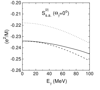
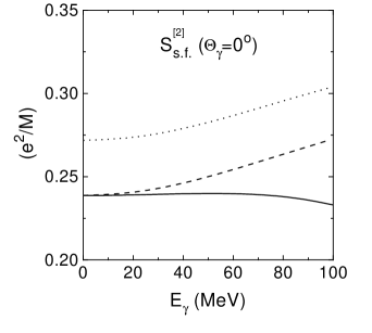
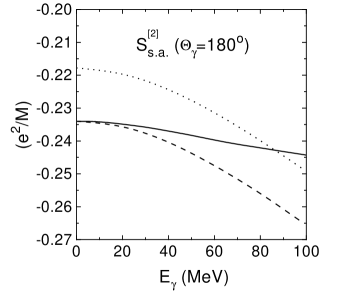
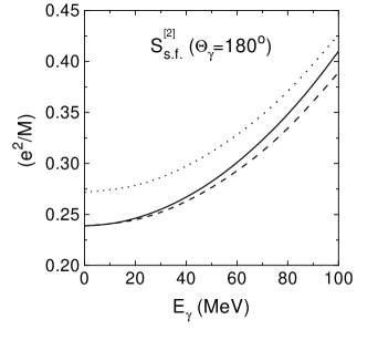
FIG. 10.: The energy dependence of the spin-averaged two-body seagull amplitude $S^{[2]}_{\rm s.a.}$ and the spin-flip amplitude $S^{[2]}_{\rm s.f.}$. Units are $e^{2}/M$. The (retarded) pion-exchange contribution is shown in dotted lines. Successive additions of heavy mesons and the $\Delta$-isobar leads to the dashed and solid lines, respectively.

The energy dependence of the two-body seagull contribution $S^{[2]}$ at forward scattering angle is illustrated in upper panels of Fig. 10. It is rather flat in the case of the spin-averaged amplitude,

$$S^{[2]}_{\rm s.a.}(E_{\gamma},0)=\frac{1}{3}\sum_{m=-1,0,1}\langle 1,m|S^{[2]}(E_{\gamma},0)|1,m\rangle,\qquad S^{[2]}_{\rm s.a.}(0,0)=-\frac{e^{2}}{2M}\,\kappa\,,$$ (127)

and it is more pronounced in the case of the spin-flip amplitude,

$$S^{[2]}_{\rm s.f.}(E_{\gamma},0)=\langle-1,1|S^{[2]}(E_{\gamma},0)|1,-1\rangle,\qquad S^{[2]}_{\rm s.f.}(0,0)=\frac{e^{2}}{M}\,\kappa_{T}\,.$$ (128)

The $\Delta$-resonance contribution becomes rather noticeable above 60 MeV, and it diminishes the energy dependence introduced by the pion exchange. As the result, the energy dependence of the seagull amplitude $S^{[2]}(E_{\gamma},0)$ gives only a 2% increase (in the absence of the polarizability contribution from the free nucleon) in the differential cross section of $\gamma d$ scattering at forward angle and $E_{\gamma}=100$ MeV.

In the bottom panels of Fig. 10 we show the spin-averaged and spin-flip two-body seagull amplitudes $S^{[2]}$ in the case of backward scattering. They are defined by equations like (127) and (128), in which $\Theta_{\gamma}=0$ is replaced by $\Theta_{\gamma}=180^{\circ}$ and the helicity of the final photon is inverted. We see that the energy dependence of the spin-flip amplitude is rather steep in this case. It increases the differential cross of deuteron Compton scattering at 100 MeV by 5% (again, in the absence of the free-nucleon polarizabilities).

In general, we have found that the effect of the $\Delta$ excitation onto the seagull amplitude $S^{[2]\pi}$ is not large. It does not exceed $-2\%$ in the differential cross section of $\gamma d$ scattering, $d\sigma/d\Omega$, at all considered energies. The two-body contribution of the $\Delta$-isobar to the resonance amplitude $R$ was found to be not large too. For example, it changes the differential cross section at 100 MeV by $+3\%$ at forward angle and by $-0.6\%$ at backward angle. At this point we disagree with the results of Ref. [37], in which it was found that the effect of the $\Delta$-excitation onto the resonance amplitude at 100 MeV is negligible at small angles and very large at $\Theta_{\gamma}\geq 90^{\circ}$ giving a $+15\%$ increase in $d\sigma/d\Omega$.

C Model dependence

Contributions of the different components $R^{\rm no\,rescat}$, $S^{[1]}$, $S^{[2]}$ and $R^{\rm rescat}$ of the total amplitude $T$ to the differential cross section at a few selected energies are shown in Fig. 11. It is seen that the effects of the resonance amplitude, the one-body seagull as well as the two-body seagull are of similar scale, though the total effect of the seagulls is more than 70% in the energy region under consideration. At the same time rescattering has a modest impact on the differential cross section. Our results confirm findings of other approaches [38, 39, 40] that the rescattering decreases the forward differential cross section and that this decrease is between 7% to 12% in the energy region of 50 to 100 MeV.

There was some discrepancy in the previous work concerning the role of $R^{\rm rescat}$ at backward angles. Weyrauch [38] found that the rescattering does not contribute at backward angles at all, whereas in the later calculations [39, 40] a visible increase in $d\sigma/d\Omega$ was claimed. Our results agree with the latter conclusions and suggest that the effect of $R^{\rm rescat}(E_{\gamma},180^{\circ})$ ranges between $+7\%$ at 50 MeV to $+3\%$ at 100 MeV. Since an accurate calculation of $R^{\rm rescat}$ is a difficult problem for our computational scheme, this finding of a relatively small effect of $R^{\rm rescat}$ at energies and angles where experimental data are available provides some justification to our approximate use of a separable potential [88] for a computation of the off-shell $T$-matrix of $NN$ rescattering.

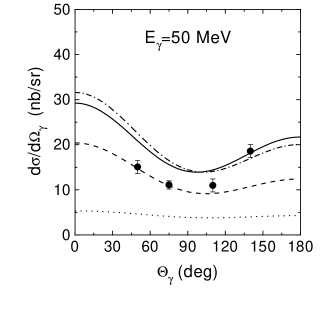
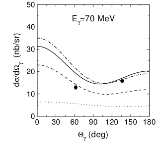
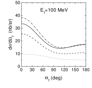
FIG. 11.: Contributions of different parts of the amplitude to the differential cross section (CM) of $\gamma d$ scattering at 50, 70, and 100 MeV. The contribution of the resonance amplitude $R^{\rm no\,rescat}$ alone is shown in dotted lines. Successive additions of the one-body seagull $S^{[1]}$, the two-body seagull $S^{[2]}$, and the rescattering amplitude $R^{\rm rescat}$ give the dashed, dash-dotted and solid lines, respectively. Nucleon polarizabilities are not included into $S^{[1]}$. Data are from Ref. [99].

An instructive feature of the calculation is that the spin-orbit (s.o.) contributions to the electromagnetic current and seagull, ${\mbox{\boldmath$\bf j$}}^{[1]\,\rm s.o.}$ and $S^{[1]\,\rm s.o.}$, which are relativistic corrections of order $1/M^{2}$ in Eqs. (36) and (38), are rather essential. Previously, it was found [96] that the spin-orbit current is responsible for the long-standing discrepancy between the theory and data on deuteron photodisintegration at forward and backward angles. In the reaction of Compton scattering, the spin-orbit interaction is important not only at extreme angles, and this importance increases with the photon energy. Either ${\mbox{\boldmath$\bf j$}}^{[1]\,\rm s.o.}$ or $S^{[1]\,\rm s.o.}$ leads to an approximately equal decrease in the differential cross section at the forward angle, and the total effect of the spin-orbit interaction on $d\sigma(E_{\gamma},0)/d\Omega$ is $-4\%$ at 50 MeV and $-15\%$ at 100 MeV. A somewhat different situation happens at the backward angle. The spin-orbit current ${\mbox{\boldmath$\bf j$}}^{[1]\,\rm s.o.}$ still decreases the differential cross section, but the spin-orbit seagull $S^{[1]\,\rm s.o.}$ makes a bigger increase. The net effect of the spin-orbit interaction at $180^{\circ}$ is $+4\%$ at 50 MeV and $+8\%$ at 100 MeV. In the central angular region of $\Theta_{\gamma}\simeq 90^{\circ}$, the spin-orbit interaction has a little impact on $d\sigma/d\Omega$ ranging between $+0.8\%$ at 50 MeV and $-0.2\%$ at 100 MeV.

Staying within the Bonn-potential picture, we have checked how the differential cross section depends on a specific choice of the potential’s parameters. The OBEPR and OBEPR(A) versions of the Bonn potential give $d\sigma/d\Omega$ which are different at most by 1% in the energy range of $50{-}100$ MeV. A bigger difference is found for the OBEPR and OBEPR(B) versions, though it decreases with the photon energy. For example, the OBEPR(B) potential gives $d\sigma/d\Omega$ which is bigger by 5% (7%) at 50 MeV and 0.5% (5%) at 100 MeV for forward (backward) angles, respectively. The main reason for such a difference comes from a very large value for the cut-off parameter $\Lambda_{\pi}=2$ GeV used in the $\pi$-exchange potential of the OBEPR(B) version, whereas $\Lambda_{\pi}=1.3$ GeV for OBEPR. Respectively, the seagull’s parameters $\kappa$ and $\kappa_{T}$ are bigger for OBEPR(B) too.

We may note that the OBEPR(B) version of the Bonn potential does not provide a satisfactory description of observables in deuteron photodisintegration [46] and thus it is not fully realistic. Therefore, one may conjecture that the sensitivity of the results on $\gamma d$ scattering would not be so noticeable if one restricts oneself to “realistic” potentials only. In this respect it is worth mentioning that the use of different momentum-space versions of the Bonn OBE potentials was found [39] to yield version-independent results for $\gamma d$ scattering within 1%.

The present results are in a qualitative agreement with our previous calculation [40] done in the framework of a “minimal model”, in which MECs and MESs are evaluated through the minimal substitution ${\mbox{\boldmath$\bf p$}}\to{\mbox{\boldmath$\bf p$}}-e{\mbox{\boldmath$\bf A$}}$ in the (Paris) $NN$ potential. As they were published, those older results did not include the spin-orbit interaction. After taking into account ${\mbox{\boldmath$\bf j$}}^{[1]\,\rm s.o.}$ and $S^{[1]\,\rm s.o.}$ the predictions of the minimal model become closer to the results of the present work, especially as for the shape of the angular dependence. Still, the minimal model gives a lower differential cross section: by 6% at 70 MeV and by 11% at 100 MeV. Such a difference can be traced in part to a weaker energy dependence of the seagull amplitude found in the minimal model and to the absence of the two-body $\Delta$-isobar effects in that model.

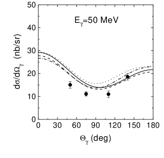
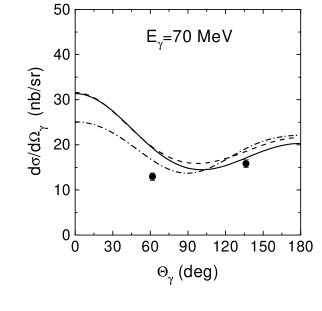
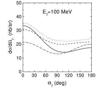
FIG. 12.: Differential cross sections (CM) of $\gamma d$ scattering. Dotted lines: Weyrauch and Arenhövel [37]. Dashed lines: Weyrauch [38]. Dash-dotted lines: Wilbois et al. [39]. Solid lines: the present work. Nucleon polarizabilities are turned off. Data are from Ref. [99].

A comparison of the present predictions with the results of other calculations of 80’s – mid 90’s [37, 38, 39] is shown in Fig. 12. There is a reasonable agreement between all the predictions at low energies like 50 MeV, maybe with the except for those of Ref. [37]. When the energy increases up to 100 MeV, we predict a bigger angular variation of $d\sigma/d\Omega$ that other works do. In fact, the discrepancy between all the results of different authors is dramatically large at 100 MeV. Moreover, since the spin-orbit interaction was not taken into account in Refs. [37, 38, 39] and since the spin-orbit effects decrease the forward cross section by 15% at 100 MeV, the genuine disagreement of other components of the scattering amplitude with those of Ref. [39] is even more serious than Fig. 12 suggests.

It is interesting that the very low differential cross section obtained by Wilbois et al. [39] at 100 MeV has found a support from a recent work of Karakowski and Miller (KM) [41], see Fig. 13. Below we mention a couple of possible reasons why the KM model disagrees with our model and shows a wrong behavior at high energies $E_{\gamma}\sim 100$ MeV. First, we have rather different effects of the spin-orbit interaction. In Ref. [41], this interaction was taken into account partly, i.e. only through the electromagnetic seagull, not through the electromagnetic current. However, it gave a much bigger decrease in the differential cross section at forward angles than that we found (cf. Fig. 12 in Ref. [41]). The second reason, perhaps less important numerically, might be that there is a mismatch between the electromagnetic and strong-interaction parts of the Hamiltonian $H_{\rm KM}$ of the KM model which destroys the gauge invariance and actually signals that some electromagnetic charges or currents in the system are missing in the theoretical formalism. The mentioned mismatch is that the electromagnetic two-body part of $H_{\rm KM}$ includes only the point-like pion-exchange piece, whereas the wave function of the deuteron is constructed using a more complicated (and more realistic) Bonn potential. The violation of the gauge invariance in the KM model did not lead to visible problems at low photon momenta $kr\ll 1$ owing to the use of the Siegert transformation which ensured automatically the fulfillment of the low-energy theorem (22). However, when $kr$ becomes large (this is the case for energies $E_{\gamma}\sim 100$ MeV), the Siegert transformation does not help, and the missing charges and/or currents can become important.

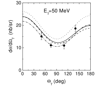
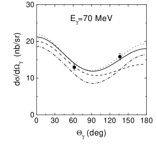
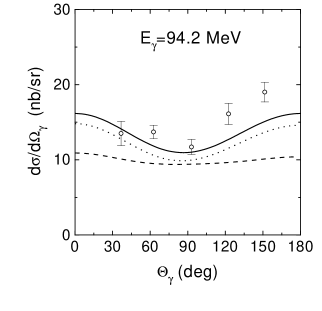
FIG. 13.: Differential cross sections (CM) of $\gamma d$ scattering. Dashed lines: Karakowski and Miller [41]. Dotted lines: Beane et al. [44]. Dash-dotted lines: Chen et al. [42]. Solid lines: the present work. Nucleon polarizabilities are included, and $\bar{\alpha}_{N}-\bar{\beta}_{N}=9$ is used for drawing the solid curves. Data are from Ref. [99] (solid circles) and Ref. [102] (open circles).

There is a simple way to verify the theoretical calculations in the particular case of $\Theta_{\gamma}=0$ and to see that the predictions of Ref. [41] at high energies are invalid. Using the Gell-Mann–Goldberger–Thirring dispersion relation jointly with the optical theorem (cf. Eq. (117)) for the spin-averaged amplitude $T_{\rm s.a.}$, we write

$$\,{\rm Re}\,T_{\rm s.a.}(\omega,0)=-\frac{Z^{2}e^{2}}{AM}+\frac{2\omega^{2}}{\pi}\,{\rm P}\int_{0}^{\infty}\frac{\sigma_{\rm tot}(\omega^{\prime})}{{\omega^{\prime}}^{2}-\omega^{2}}\,d\omega^{\prime},$$ (129)

where $\sigma_{\rm tot}$ is the total photoabsorption cross section. Keeping in mind that the total cross section of meson production off the deuteron is dominated by meson production off quasi-free nucleons, we see that this part of the photoabsorption cross section is responsible for the component of the $\gamma d$ scattering amplitude which is related with the polarizabilities of free nucleons (up to relatively small effects due to medium modifications of these polarizabilities). Therefore, subtracting the meson-production part of the photoabsorption cross section and keeping in Eq. (129) non-mesonic, or photodisintegration part of the cross section, we can approximately identify the resulting r.h.s. of Eq. (129) with the $\gamma d$ scattering amplitude, in which the internal (mesonic) structure of the nucleon is disregarded. In other words, using the deuteron photodisintegration cross section $\sigma^{\gamma d\to pn}_{\rm tot}$ instead of $\sigma_{\rm tot}$ in Eq. (129), we should obtain the $\gamma d$ scattering amplitude with point-like nucleons having zero polarizability. See Ref. [6] for a more detailed discussion of these steps.

We have evaluated the integral in Eq. (129) at energies $\omega\lesssim 100$ MeV using: (i) the effective-range parameterization of $\sigma^{\gamma d\to pn}_{\rm tot}(\omega^{\prime})$ at energies $\omega^{\prime}$ below 20 MeV (see Ref. [100], Eq. (2.18)) which gives an accurate description of experimental data at low energies, and (ii) a phenomenological fit [101] to available experimental data between 20 and 440 MeV. At higher $\omega^{\prime}$, the photodisintegration cross section is small and can be safely neglected in the integral. The result of such an evaluation of Eq. (129) is shown in Fig. (14) by the solid curve, together with our predictions (dashed line) based on the Bonn-potential picture, in which the nucleon polarizabilities are disregarded. Generally, we find very good agreement between the two curves. Some disagreement of about 6% at very low energies appears due to an approximate way of finding the rescattering amplitude $R^{\rm rescat}$, as it was already mentioned in Section V. At energies above 10 MeV, the rescattering amplitude is less important, and the agreement between the two calculations improves. It is better that 3% even at 100 MeV. It is needless to say that the Bonn-potential picture nicely reproduces the experimental data on the total cross section $\sigma^{\gamma d\to pn}_{\rm tot}$ at all energies below pion threshold as well as the differential cross section of deuteron photodisintegration and polarization observables [46].

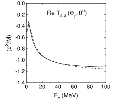
FIG. 14.: The spin-averaged amplitude of forward $\gamma d$-scattering. Solid line: the r.h.s. of Eq. (129). Dashed line: results of the present work based on the Bonn potential. Meson photoproduction and nucleon polarizabilities are disregarded.

Now let us compare our predictions with those obtained within two different flavors of effective field theory (EFT) for few-nucleon systems [42, 44] (a general review of the EFT approach to nuclear problems can be found in Ref. [103]). At “high” energies $E_{\gamma}\sim 70{-}100$ MeV, we have a qualitative agreement with the results of Beane et al. [44], who used the so-called Weinberg formulation of the nuclear EFT. See Fig. 13 for a comparison. In part, a proximity of our and Beane et al. predictions is caused by their use of a realistic wave function to evaluate matrix elements of the ChPT kernel, the latter denoting the amplitude of $\gamma NN\to\gamma NN$ taken to order ${\cal O}(Q^{3})$ in the chiral perturbation theory expansion. It was actually the wave function of the Bonn potential. Furthermore, the dominating part of the two-body seagull operator is the same in our two approaches. It comes from the retarded pion exchange. Despite the Bonn-potential picture uses form factors in the $\pi NN$ vertices and additional heavier mesons (to make improvements to the potential at small distances), the effects of the form factor and the heavy mesons onto the seagull amplitude are reduced to some changes of $\kappa$ which almost cancel each other. Specifically, we have found $\kappa=0.48-0.04+0.03$, where the three numbers are the contribution of the pure pion exchange, the contribution from the fictitious $\Lambda$ particle simulating the $\pi NN$ form factor (see Section IV), and the contribution of $\rho$, $\omega$, $\delta$ and $\sigma$ mesons, respectively.

We can notice that all the contributions counted in Ref. [44] have been taken into account in our calculation as well. Beyond that, we included other corrections which formally belong to higher orders in $Q$ in the power counting scheme of the EFT but are large numerically. An instructive example is the amplitude $R^{\rm no\,rescat}$ given by Eq. (103), in which each of the amplitudes of the $\gamma d\to pn$ transitions is dominated, at high energies, by the pion-exchange current ${\mbox{\boldmath$\bf j$}}^{[2]\,\pi}$, as shown in Fig. 9. This rather large contribution formally appears only in order ${\cal O}(Q^{5})$ of the power counting scheme of Ref. [44].

A resemblance of the two predictions seems to be lost at lower energies, where the scattering amplitude of Beane et al. begins to deviate from the correct value fixed, for instance, by the dispersion relation (129) at the forward angle. Such a failure is not a surpise and it was anticipated in Ref. [44] as a result of contributions from the $NN$ intermediate states which break down the used power counting at low energies.

It is worth mentioning that the evaluation of matrix elements of the ChPT kernel between phenomenological (Bonn or Nijmegen) wave functions, which are not consistent with the one-pion-exchange dynamics of the $NN$ interaction incorporated into the ChPT kernel, automatically means the absence of the gauge invariance in the scheme of Ref. [44]. This itself is a sufficient reason for a failure of such a theory at very low energies where the gauge invariance is crucial.

In view of close magnitudes of $\kappa$ arising in our approach and in that of Ref. [44], we can conjecture that the main difference between the two predictions at energies of about 100 MeV is related with our taking into account the $\Delta$-resonance excitation (both in one-body and two-body operators) and with our taking into account the contribution $R^{\rm no\,rescat}$ (of the correct magnitude) and the contribution $R^{\rm rescat}$.

The problem with the gauge invariance and with the region of very low energies does not exist in the version of EFT used by Chen et al. [42]. Their work is based on the so-called Kaplan–Savage–Wise (KSW) regularization which successfully resolves the problem of a poor power-series convergence in the case of large $s$-wave $NN$-scattering lengths [104]. $NN$ rescattering contributions are accurately taken into account in that approach. However, even being quite accurate at low energies, this approach becomes inapplicable when the momenta of nucleons in the rescattering diagrams exceed the range of convergence of power series which is about $\Lambda_{NN}=16\pi M/g_{\pi NN}^{2}\simeq 300$ MeV. This makes predictions of Ref. [42] not well controlled at energies $\gtrsim 70{-}90$ MeV. Therefore, there is no surprise that these predictions at 70 MeV lie visibly lower than our predictions (and those of Beane et al. [44]), including the $\Theta_{\gamma}=0$ point, where the dispersion relation (129) strongly favors our calculation. It is worth mentioning that neither $\Delta$-isobar excitation nor the spin-orbit current and seagull are taken into account in Ref. [42] since these pieces appear only in higher orders of the used expansion.

D Determination of the nucleon polarizabilities

Considering the nucleon dipole polarizabilities $\bar{\alpha}_{N}$ and $\bar{\beta}_{N}$ in the electromagnetic seagull operator (38) as free parameters, we can check the sensitivity of the differential cross section $d\sigma/d\Omega$ with respect to variation of these parameters. Our results are shown in Fig. 15 together with a few experimental data available from Urbana ($E_{\gamma}=49$ and 69 MeV) [99] and Saskatoon ($E_{\gamma}=94$ MeV) [102]. We do not show how the differential cross section depends on the sum of the electric and magnetic polarizability, because this sum is reasonably-well fixed by the Baldin sum rule, Eq. (50). As for the difference of $\bar{\alpha}_{N}$ and $\bar{\beta}_{N}$ which is not well-known theoretically, it can be determined from data at large scattering angle.

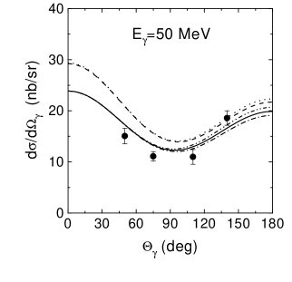
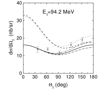
FIG. 15.: Dependence of the differential cross section (CM) of $\gamma d$ scattering on the nucleon-averaged dipole polarizabilities $\bar{\alpha}_{N}$ and $\bar{\beta}_{N}$. Dashed lines: all the polarizabilities (including those of higher order) are turned off. Dotted lines: only higher-order polarizabilities, Eq. (53), are included. Dashed-double-dotted, solid, and dashed-dotted lines: $\bar{\alpha}_{N}-\bar{\beta}_{N}=6$, 9 and 12, respectively, $\bar{\alpha}_{N}+\bar{\beta}_{N}=14.6$ is fixed, and the higher-order polarizabilities are included. Data are from Ref. [99] (solid circles) and Ref. [102] (open circles).

Of course, the highest sensitivity is observed at the highest photon energy. Nevertheless, we believe that data at medium energies like 70 MeV are also quite useful, because theoretical uncertainties in our computation related, for example, with omitted relativistic corrections or with omitted dispersion effects due to two-pion exchanges are expected to be smaller at lower energies.

Dotted lines in Fig. 15 illustrate the fact that the higher-order polarizabilities (53) are in no way negligible when the nucleon dipole polarizabilities are determined from $\gamma d$ scattering at energies $\gtrsim 70$ MeV. This feature was paid attention to also in Ref. [44], in which the higher-order contributions appeared as an intrinsic part of the one-pion-loop diagrams of the ChPT kernel. Since, however, we use the higher-order polarizabilities which are given by dispersion relations [25, 62, 69, 67] and which are very different from those suggested by the one-pion-loop mechanism (in part, due to the $\Delta$-contribution, see Ref. [25]), we predict a much bigger effect at backward angles.

A straightforward two-parameter fit of the Urbana data [99] gives $\bar{\alpha}_{N}=14.5\pm 2.7$ and $\bar{\beta}_{N}=6.6\pm 2.7$, whereas a similar fit of the Saskatoon data [102] gives a lower value of the electric polarizability: $\bar{\alpha}_{N}=8.4\pm 1.8$ and $\bar{\beta}_{N}=6.2\pm 1.8$. Making a combined fit of all the data, we obtain

$$\bar{\alpha}_{N}+\bar{\beta}_{N}=17.1\pm 1.6,$$ (130)

what is in agreement with the theoretical expectation (50), and

$$\bar{\alpha}_{N}-\bar{\beta}_{N}=4.0\pm 1.5,$$ (131)

though with a poor $\chi^{2}/N_{\rm d.o.f.}=21/9$. Systematic uncertainties of the experimental data are included into the obtained estimates (130) and (131). However, it is not so easy to estimate uncertainties introduced by the theoretical model. Certainly, they are not less than the experimental uncertainties.

Taken as they are, these numbers, together with the experimental data on the polarizabilities of the proton (2) can be considered as an indication that the electric polarizability of the neutron is $\bar{\alpha}_{n}=9\pm 3$, and the neutron magnetic polarizability is $\bar{\beta}_{n}=11\pm 3$. While the obtained sum $\bar{\alpha}_{n}+\bar{\beta}_{n}=20\pm 3$ reasonably agrees with the theoretical estimate (49), the obtained difference $\bar{\alpha}_{n}-\bar{\beta}_{n}=-2\pm 3$ is rather far from both the similar difference in the proton case found experimentally, $\bar{\alpha}_{p}-\bar{\beta}_{p}=10\pm 2$ [12, 16], and from theoretical estimates based on dispersion relations which predict roughly $\bar{\alpha}_{n}-\bar{\beta}_{n}\simeq\bar{\alpha}_{p}-\bar{\beta}_{p}$ (see, e.g., Refs. [1, 3, 68]). It is clear that a further experimental and theoretical work is needed to reduce the uncertainties. New data can appear from Lund [105].

Among other observables of $\gamma d$ scattering which are sensitive to the nucleon polarizabilities too, we briefly discuss the beam asymmetry $\Sigma$, Eq. (113). In Fig. 16 we show how different components of the Compton scattering amplitude affect $\Sigma$ (this is helpful for imagining a possible scale of model uncertainties) and how $\Sigma$ is sensitive to the nucleon polarizabilities. One can notice a strong dominance of the one-body seagull amplitude, whereas the role of the two-body seagull contribution is smaller than that in the case of the differential cross section. The role of $NN$ rescattering is again small.

The spin-orbit interaction essentially affects $\Sigma$ and gives a 10% increase at central angles. It mainly comes through the one-body seagull amplitude $S^{[1]}$. The contribution of the $\Delta$ excitation to the two-body seagull amplitude $S^{[2]\pi}$ changes the beam asymmetry by less than 1%, but the $\Delta$ contribution into the resonance amplitude $R$ is rather visible, reducing $\Sigma$ by 6% at 100 MeV. Pion-retardation effects have only a tiny impact on $\Sigma$. The use of the potential OBEPR(B) instead of OBEPR has a big effect and reduces $\Sigma$ by 14% at 100 MeV.

It looks like experiments with the linearly-polarized photon beam can also be useful for measuring the nucleon polarizabilities, provided the accuracy of measurements is better than $\sim 5{-}10\%$.

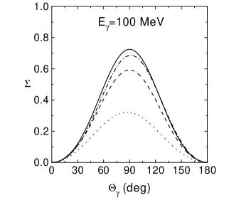
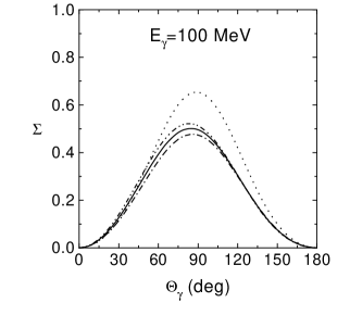
FIG. 16.: Left panel: Contributions of different parts of the Compton scattering amplitude to the beam asymmetry at 100 MeV. Notation of curves is as in Fig. 11. Right panel: Dependence of the beam asymmetry on the nucleon-averaged dipole polarizabilities $\bar{\alpha}_{N}$ and $\bar{\beta}_{N}$. Notation of curves is as in Fig. 15.

We conclude saying that the reaction of deuteron Compton scattering at energies of about 50–100 MeV has a great potential for a determination of the electromagnetic polarizabilities of the neutron. Currently, the available theoretical models show a big divergence in their results, in part because they do not take into account all important contributions. So, a further theoretical work is needed to improve the accuracy of the models before any firm conclusions could be inferred about the values of $\bar{\alpha}_{N}$ and $\bar{\beta}_{N}$. Better experimental data are also needed to this aim.

A Electromagnetic seagulls from heavy mesons of the OBE potential

In this appendix we give explicit formulas for the seagulls $S_{ij}^{\alpha}$ produced by the meson exchanges $\alpha=\eta$, $\sigma$, $\delta$, $\omega$ and $\rho$ of the Bonn potential (OBEPR). All of them are obtained through a direct evaluation of the diagrams shown in Fig. 1c. The electromagnetic effective meson-nucleon vertices $\gamma\alpha NN$ and $\gamma\gamma\alpha NN$ in these diagrams arise from the relativistic boson-nucleon effective Lagrangian of Refs. [73, 74], in which a nonrelativistic reduction is done and terms up to order ${\cal O}(M^{-2})$ are only retained. Such a procedure is consistent with the whole construction of the OBEPR, because this potential itself is built through the truncation of the relativistic Feynman diagrams of the one-boson exchanges to order ${\cal O}(M^{-2})$ (see Ref. [74], Appendix A.3).

Technically, the nonrelativistic reduction can be conveniently performed [81] by considering appropriate relativistic Feynman diagrams (see Fig. 17) and keeping only the negative-energy part $P_{-}$ of the nucleon propagators. To leading order in $1/M$, it is sufficient to take $P_{-}$ in the static limit, i.e.

$$P_{-}=-\frac{1}{2M}\pmatrix{0&0\cr 0&1}.$$ (A1)

It is worth noticing that the contact vertex $\gamma\alpha NN$ in Fig. 17 appears only in the case of $\alpha=\rho$, being caused by the tensor coupling of the charged $\rho$-meson to the nucleon. In the formalism of the pseudo-scalar $\pi NN$ coupling used in Refs. [73, 74], the contact vertex $\gamma\pi NN$ is absent.

FIG. 17.: Effective contact meson-nucleon vertices $\gamma\alpha NN$ (diagrams a) and $\gamma\gamma\alpha NN$ (diagrams b) arising from the antinucleon degrees of freedom. Thick lines denote the negative-energy part $P_{-}$ of the nucleon propagator, Eq. (A1).

We use the same notation as in Section IV. In particular, the momenta ${\mbox{\boldmath$\bf q$}}_{1}$, ${\mbox{\boldmath$\bf q$}}_{2}$, ${\mbox{\boldmath$\bf K$}}_{1}$ and ${\mbox{\boldmath$\bf K$}}_{2}$ are defined by Eqs. (70) and (78). We introduce also the vectors

$${\mbox{\boldmath$\bf P$}}_{1}={\mbox{\boldmath$\bf p$}}_{1}+{\mbox{\boldmath$\bf p$}}^{\prime}_{1},\quad{\mbox{\boldmath$\bf P$}}_{2}={\mbox{\boldmath$\bf p$}}_{2}+{\mbox{\boldmath$\bf p$}}^{\prime}_{2}.$$ (A2)

The functions $G_{\alpha}({\mbox{\boldmath$\bf q$}})$, $G_{1\alpha}({\mbox{\boldmath$\bf q$}}_{1},{\mbox{\boldmath$\bf q$}}_{2})$, $G_{2\alpha}({\mbox{\boldmath$\bf q$}}_{1},{\mbox{\boldmath$\bf q$}}_{2},{\mbox{\boldmath$\bf K$}})$, and $D_{\alpha}({\mbox{\boldmath$\bf q$}}_{1},{\mbox{\boldmath$\bf q$}}_{2},{\mbox{\boldmath$\bf K$}}_{1},{\mbox{\boldmath$\bf K$}}_{2})$ used below are defined as in Section IV with the evident replacement $\pi\to\alpha$ in all masses $m_{\alpha}$ and cutoff parameters $\Lambda_{\alpha}$. The constants $\kappa_{\alpha}$ denote the ratios of the tensor and vector coupling constants for the $\omega NN$ and $\rho NN$ vertices, $\kappa_{\alpha}=f_{\alpha}/g_{\alpha}$.

Evaluating the diagrams in Figs. 1c and 17, we obtain the following results.

$\bullet$ Isoscalar exchanges:

$$\epsilon_{i}^{\prime*}\epsilon_{j}S_{ij}^{\eta}(-{\mbox{\boldmath$\bf k$}}^{\prime},{\mbox{\boldmath$\bf k$}};{\mbox{\boldmath$\bf p$}}^{\prime}_{1},{\mbox{\boldmath$\bf p$}}^{\prime}_{2};{\mbox{\boldmath$\bf p$}}_{1},{\mbox{\boldmath$\bf p$}}_{2})=0,$$ (A3)

$$\epsilon_{i}^{\prime*}\epsilon_{j}S_{ij}^{\sigma}(-{\mbox{\boldmath$\bf k$}}^{\prime},{\mbox{\boldmath$\bf k$}};{\mbox{\boldmath$\bf p$}}^{\prime}_{1},{\mbox{\boldmath$\bf p$}}^{\prime}_{2};{\mbox{\boldmath$\bf p$}}_{1},{\mbox{\boldmath$\bf p$}}_{2})=-{\mbox{\boldmath$\bf\epsilon$}}\cdot{\mbox{\boldmath$\bf\epsilon$}}^{\prime*}\,\frac{e^{2}g_{\sigma}^{2}}{2M^{2}}\Big{[}Z_{1}G_{\sigma}({\mbox{\boldmath$\bf q$}}_{2})+(1\leftrightarrow 2)\Big{]},$$ (A4)

$$\epsilon_{i}^{\prime*}\epsilon_{j}S_{ij}^{\omega}(-{\mbox{\boldmath$\bf k$}}^{\prime},{\mbox{\boldmath$\bf k$}};{\mbox{\boldmath$\bf p$}}^{\prime}_{1},{\mbox{\boldmath$\bf p$}}^{\prime}_{2};{\mbox{\boldmath$\bf p$}}_{1},{\mbox{\boldmath$\bf p$}}_{2})=-{\mbox{\boldmath$\bf\epsilon$}}\cdot{\mbox{\boldmath$\bf\epsilon$}}^{\prime*}\,\frac{e^{2}g_{\omega}^{2}}{2M^{2}}\Big{[}Z_{1}G_{\omega}({\mbox{\boldmath$\bf q$}}_{2})-2Z_{1}Z_{2}G_{\omega}({\mbox{\boldmath$\bf K$}}_{1})+(1\leftrightarrow 2)\Big{]}.$$ (A5)

Writing the last equation, we have used that $\kappa_{\omega}=0$ for the Bonn potential.

$\bullet$ Isovector exchanges:

$$\epsilon_{i}^{\prime*}\epsilon_{j}S_{ij}^{\delta}(-{\mbox{\boldmath$\bf k$}}^{\prime},{\mbox{\boldmath$\bf k$}};{\mbox{\boldmath$\bf p$}}^{\prime}_{1},{\mbox{\boldmath$\bf p$}}^{\prime}_{2};{\mbox{\boldmath$\bf p$}}_{1},{\mbox{\boldmath$\bf p$}}_{2})=-{\mbox{\boldmath$\bf\epsilon$}}\cdot{\mbox{\boldmath$\bf\epsilon$}}^{\prime*}\,\frac{e^{2}g_{\delta}^{2}}{2M^{2}}\Big{[}Z_{1}\tau_{2}^{z}G_{\delta}({\mbox{\boldmath$\bf q$}}_{2})+(1\leftrightarrow 2)\Big{]}$$ (A6)

$$\qquad{}+\frac{e^{2}g_{\delta}^{2}}{4M^{2}}\Big{\{}\Big{(}{\mbox{\boldmath$\bf q$}}_{2}\cdot{\mbox{\boldmath$\bf\epsilon$}}^{\prime*}G_{1\delta}({\mbox{\boldmath$\bf q$}}_{2},{\mbox{\boldmath$\bf K$}}_{1})\Big{[}T_{12}({\mbox{\boldmath$\bf q$}}_{1}\cdot{\mbox{\boldmath$\bf\epsilon$}}+i{\mbox{\boldmath$\bf\sigma$}}_{1}\times{\mbox{\boldmath$\bf P$}}_{1}\cdot{\mbox{\boldmath$\bf\epsilon$}})$$ (A7)

$$\qquad\qquad{}+i({\mbox{\boldmath$\bf\tau$}}_{1}\times{\mbox{\boldmath$\bf\tau$}}_{2})^{z}\,({\mbox{\boldmath$\bf P$}}_{1}\cdot{\mbox{\boldmath$\bf\epsilon$}}+i{\mbox{\boldmath$\bf\sigma$}}_{1}\times{\mbox{\boldmath$\bf q$}}_{1}\cdot{\mbox{\boldmath$\bf\epsilon$}})\Big{]}+(1\leftrightarrow 2)\Big{)}$$ (A8)

$$\qquad\qquad\qquad{}+({\mbox{\boldmath$\bf\epsilon$}}\leftrightarrow{\mbox{\boldmath$\bf\epsilon$}}^{\prime*},~{}{\mbox{\boldmath$\bf K$}}_{1}\leftrightarrow-{\mbox{\boldmath$\bf K$}}_{2})\Big{\}}$$ (A9)

$$\qquad{}-e^{2}g_{\delta}^{2}\,T_{12}D_{\delta}({\mbox{\boldmath$\bf q$}}_{1},{\mbox{\boldmath$\bf q$}}_{2},{\mbox{\boldmath$\bf K$}}_{1},{\mbox{\boldmath$\bf K$}}_{2})\Big{[}1-\frac{{\mbox{\boldmath$\bf P$}}_{1}^{2}+{\mbox{\boldmath$\bf P$}}_{2}^{2}-{\mbox{\boldmath$\bf q$}}_{1}^{2}-{\mbox{\boldmath$\bf q$}}_{2}^{2}}{16M^{2}}$$ (A10)

$$\qquad\qquad\qquad\qquad{}-i\frac{{\mbox{\boldmath$\bf\sigma$}}_{1}\times{\mbox{\boldmath$\bf q$}}_{1}\cdot{\mbox{\boldmath$\bf P$}}_{1}+{\mbox{\boldmath$\bf\sigma$}}_{2}\times{\mbox{\boldmath$\bf q$}}_{2}\cdot{\mbox{\boldmath$\bf P$}}_{2}}{8M^{2}}\Big{]},$$ (A11)

$$\epsilon_{i}^{\prime*}\epsilon_{j}S_{ij}^{\rho}(-{\mbox{\boldmath$\bf k$}}^{\prime},{\mbox{\boldmath$\bf k$}};{\mbox{\boldmath$\bf p$}}^{\prime}_{1},{\mbox{\boldmath$\bf p$}}^{\prime}_{2};{\mbox{\boldmath$\bf p$}}_{1},{\mbox{\boldmath$\bf p$}}_{2})=-{\mbox{\boldmath$\bf\epsilon$}}\cdot{\mbox{\boldmath$\bf\epsilon$}}^{\prime*}\,\frac{e^{2}g_{\rho}^{2}}{2M^{2}}\Big{[}(Z_{1}\tau_{2}^{z}-\kappa_{\rho}T_{12})G_{\rho}({\mbox{\boldmath$\bf q$}}_{2})+(1\leftrightarrow 2)\Big{]}$$ (A12)

$$\qquad{}+\frac{e^{2}g_{\rho}^{2}}{4M^{2}}\Big{\{}G_{\rho}({\mbox{\boldmath$\bf K$}}_{1})\Big{[}{\mbox{\boldmath$\bf\epsilon$}}\cdot{\mbox{\boldmath$\bf\epsilon$}}^{\prime*}(T_{12}-4Z_{1}Z_{2})+(1+\kappa_{\rho})^{2}\,T_{12}\,{\mbox{\boldmath$\bf\sigma$}}_{1}\times{\mbox{\boldmath$\bf\epsilon$}}\cdot{\mbox{\boldmath$\bf\sigma$}}_{2}\times{\mbox{\boldmath$\bf\epsilon$}}^{\prime*}$$ (A13)

$$\qquad\qquad\qquad{}-(1+\kappa_{\rho})({\mbox{\boldmath$\bf\tau$}}_{1}\times{\mbox{\boldmath$\bf\tau$}}_{2})^{z}\,({\mbox{\boldmath$\bf\sigma$}}_{1}+{\mbox{\boldmath$\bf\sigma$}}_{2})\cdot{\mbox{\boldmath$\bf\epsilon$}}^{\prime*}\times{\mbox{\boldmath$\bf\epsilon$}}\Big{]}+(1\leftrightarrow 2)\Big{\}}$$ (A14)

$$\qquad{}+\frac{e^{2}g_{\rho}^{2}}{4M^{2}}\Bigg{[}\Big{(}{\mbox{\boldmath$\bf q$}}_{2}\cdot{\mbox{\boldmath$\bf\epsilon$}}^{\prime*}G_{1\rho}({\mbox{\boldmath$\bf q$}}_{2},{\mbox{\boldmath$\bf K$}}_{1})\Big{\{}T_{12}\Big{[}(1+4\kappa_{\rho}){\mbox{\boldmath$\bf q$}}_{1}\cdot{\mbox{\boldmath$\bf\epsilon$}}+i(1+2\kappa_{\rho}){\mbox{\boldmath$\bf\sigma$}}_{1}\times{\mbox{\boldmath$\bf P$}}_{1}\cdot{\mbox{\boldmath$\bf\epsilon$}}$$ (A15)

$$\qquad\qquad\qquad\qquad{}-2i(1+\kappa_{\rho}){\mbox{\boldmath$\bf\sigma$}}_{1}\times{\mbox{\boldmath$\bf P$}}_{2}\cdot{\mbox{\boldmath$\bf\epsilon$}}-2(1+\kappa_{\rho})^{2}\,{\mbox{\boldmath$\bf\sigma$}}_{1}\times{\mbox{\boldmath$\bf\epsilon$}}\cdot{\mbox{\boldmath$\bf\sigma$}}_{2}\times{\mbox{\boldmath$\bf q$}}_{2}\Big{]}$$ (A16)

$$\qquad\qquad{}+i({\mbox{\boldmath$\bf\tau$}}_{1}\times{\mbox{\boldmath$\bf\tau$}}_{2})^{z}\,\Big{[}({\mbox{\boldmath$\bf P$}}_{1}-2{\mbox{\boldmath$\bf P$}}_{2})\cdot{\mbox{\boldmath$\bf\epsilon$}}+i(1+2\kappa_{\rho}){\mbox{\boldmath$\bf\sigma$}}_{1}\times{\mbox{\boldmath$\bf q$}}_{1}\cdot{\mbox{\boldmath$\bf\epsilon$}}-2i(1+\kappa_{\rho}){\mbox{\boldmath$\bf\sigma$}}_{2}\times{\mbox{\boldmath$\bf q$}}_{2}\cdot{\mbox{\boldmath$\bf\epsilon$}}\Big{]}\Big{\}}$$ (A17)

$$\qquad\qquad\qquad\qquad{}+(1\leftrightarrow 2)\Big{)}+({\mbox{\boldmath$\bf\epsilon$}}\leftrightarrow{\mbox{\boldmath$\bf\epsilon$}}^{\prime*},~{}{\mbox{\boldmath$\bf K$}}_{1}\leftrightarrow-{\mbox{\boldmath$\bf K$}}_{2})\Bigg{]}$$ (A18)

$$\qquad{}+e^{2}g_{\delta}^{2}\,T_{12}D_{\rho}({\mbox{\boldmath$\bf q$}}_{1},{\mbox{\boldmath$\bf q$}}_{2},{\mbox{\boldmath$\bf K$}}_{1},{\mbox{\boldmath$\bf K$}}_{2})\Bigg{[}1+\frac{{\mbox{\boldmath$\bf P$}}_{1}^{2}+{\mbox{\boldmath$\bf P$}}_{2}^{2}-4{\mbox{\boldmath$\bf P$}}_{1}\cdot{\mbox{\boldmath$\bf P$}}_{2}}{16M^{2}}+(1-4\kappa_{\rho})\frac{{\mbox{\boldmath$\bf q$}}_{1}^{2}+{\mbox{\boldmath$\bf q$}}_{2}^{2}}{16M^{2}}$$ (A19)

$$\qquad\qquad\qquad{}+i(1+2\kappa_{\rho})\,\frac{{\mbox{\boldmath$\bf\sigma$}}_{1}\times{\mbox{\boldmath$\bf q$}}_{1}\cdot{\mbox{\boldmath$\bf P$}}_{1}+{\mbox{\boldmath$\bf\sigma$}}_{2}\times{\mbox{\boldmath$\bf q$}}_{2}\cdot{\mbox{\boldmath$\bf P$}}_{2}}{8M^{2}}$$ (A20)

$$\qquad\qquad\qquad{}-i(1+\kappa_{\rho})\,\frac{{\mbox{\boldmath$\bf\sigma$}}_{1}\times{\mbox{\boldmath$\bf q$}}_{1}\cdot{\mbox{\boldmath$\bf P$}}_{2}+{\mbox{\boldmath$\bf\sigma$}}_{2}\times{\mbox{\boldmath$\bf q$}}_{2}\cdot{\mbox{\boldmath$\bf P$}}_{1}}{4M^{2}}$$ (A21)

$$\qquad\qquad\qquad\qquad{}+(1+\kappa_{\rho})^{2}\,\frac{{\mbox{\boldmath$\bf\sigma$}}_{1}\times{\mbox{\boldmath$\bf q$}}_{1}\cdot{\mbox{\boldmath$\bf\sigma$}}_{2}\times{\mbox{\boldmath$\bf q$}}_{2}}{4M^{2}}\Bigg{]}.$$ (A22)

Writing Eqs. (A6) and (A12), we used the radiation gauge (23).

With the help of Eqs. (71) and (85), one can verify that thus constructed seagull operators $S_{ij}^{\alpha}$ satisfy the equation (87), provided the electromagnetic currents ${\mbox{\boldmath$\bf j$}}^{\alpha}$ are taken as obtained [46] from the same boson exchanges to order ${\cal O}(M^{-2})$.

Numerical values of the masses $m_{\alpha}$, the couplings $g_{\alpha}$ (as well as $\kappa_{\alpha}$ for the vector mesons), and the cutoff parameters $\Lambda_{\alpha}$ for different bosons are taken exactly the same as for the Bonn potential (OBEPR) itself [73, 74]. The only exception concerns the $\sigma$-exchange. The matter is that the Bonn parameterization of the $\sigma$-exchange suggests to use a different mass $m_{\sigma}$ and the coupling $g_{\sigma}$ for different $NN$ channels with the total isospin $I=0$ or $I=1$. We found this feature inconvenient for building electromagnetic operators which mix the isospin. Since we noticed no visible distinction between our predictions using $\sigma$-MEC and $\sigma$-MES with either of the two sets of ($m_{\sigma}$, $g_{\sigma}$), we took for the sake of simplicity the $\sigma$-meson parameters proposed by the Bonn group for the $I=0$ channel.

As a final comment we have to mention that, strictly speaking, the nonrelativistic reduction of the Feynman diagrams to order ${\cal O}(M^{-2})$ considered as a method of a determination of the OBE potentials $V^{\alpha}$, the OBE electromagnetic currents $j_{\mu}^{\alpha}$, and the OBE electromagnetic seagulls $S_{\mu\nu}^{\alpha}$ may need a further refinement. The matter is that the operators obtained in this way are manifestly frame-dependent. Specifically, they explicitly depend on the individual momenta of the nucleons, ${\mbox{\boldmath$\bf P$}}_{1}$ and ${\mbox{\boldmath$\bf P$}}_{2}$, rather than on the relative variable ${\mbox{\boldmath$\bf P$}}_{1}-{\mbox{\boldmath$\bf P$}}_{2}$ (see, e.g., Eqs. (A6), (A12) and also Ref. [46]). This is not what is expected for potentials, MEC, and MES in the nonrelativistic framework.

It is possible to propose a modification of the diagrammatic representation of the boson exchanges which leads to Galilei-invariant results and to some changes in the above equations for MEC and MES [106]. We checked, however, that such a modification has only a minor numerical effect and can be neglected in the present context.

REFERENCES

- [1] V.A. Petrun’kin, Fiz. Elem. Chast. At. Yad. 12 (1981) 692 [Sov. J. Part. Nucl. 12 (1981) 278].
- [2] H. Arenhövel, in New Vistas in Electro-Nuclear Physics, eds. E.L. Tomusiak, H.S. Caplan and E.T. Dressler (Plenum Press, 1986), p. 251.
- [3] A.I. L’vov, Int. J. Mod. Phys. A 8 (1993) 5267.
- [4] V. Bernard, N. Kaiser and U.-G. Meissner, Int. J. Mod. Phys. E 4 (1995) 193.
- [5] Proc. Workshop on Chiral Dynamics: Theory and Experiment, Mainz, 1997, eds. A. Bernstein, D. Drechsel and Th. Walcher (Lecture Notes in Physics, v. 513, Springer, 1998).
- [6] M.-Th. Hütt, A.I. L’vov, A.I. Milstein and M. Schumacher, Phys. Reports 323 (2000) 457.
- [7] V.I. Goldansky, O.A. Karpukhin, A.V. Kutsenko and V.V. Pavlovskaya, Nucl. Phys. 18 (1960) 473.
- [8] P. Baranov, G. Buinov, V. Godin, V. Kuznetzova, V. Petrun’kin, L. Tatarinskaya, V. Shirtchenko, L. Shtarkov, V. Yurtchenko and Yu. Yanulis, Phys. Lett. B 52 (1974) 122.
- [9] F.J. Federspiel, R.A. Eisenstein, M.A. Lucas, B.E. MacGibbon, K. Mellendorf, A.M. Nathan, A. O’Neill and D.P. Wells, Phys. Rev. Lett. 67 (1991) 1511.
- [10] A. Zieger, R. Van de Vyver, D. Christmann, A. De Graeve, C. Van den Abeele and B. Ziegler, Phys. Lett. B 278 (1992) 34.
- [11] E.L. Hallin, D. Amendt, J.C. Bergstrom, H.S. Caplan, R. Igarashi, D.M. Skopik, E.C. Booth, D. Delli Carpini, J.P. Miller, F.J. Federspiel, B.E. MacGibbon and A.M. Nathan, Phys. Rev. C 48 (1993) 1497.
- [12] B.E. MacGibbon, G. Garino, M.A. Lucas, A.M. Nathan, G. Feldman and B. Dolbilkin, Phys. Rev. C 52 (1995) 2097.
- [13] J. Tonnison, A.M. Sandorfi, S. Hoblit and A.M. Nathan, Phys. Rev. Lett. 80 (1998) 4382.
- [14] A.M. Baldin, Nucl. Phys. 18 (1960) 310.
- [15] L.I. Lapidus, Zh. Eksp. Teor. Fiz. 43 (1962) 1358 [Sov. Phys. JETP 16 (1963) 964].
- [16] P.S. Baranov, A.I. L’vov, V.A. Petrun’kin and L.N. Shtarkov, Lebedev Physical Institute, preprint No. 50 (1999) [in Russian].
- [17] Yu.A. Alexandrov, Fundamental properties of the neutron (Clarendon Press, Oxford, 1992).
- [18] R.M. Thaler, Phys. Rev. 114 (1959) 827.
- [19] A.I. L’vov, Lebedev Physical Institute, preprint No. 344 (1987).
- [20] J. Schmiedmayer, P. Riehs, J.A. Harvey and N.W. Hill, Phys. Rev. Lett. 66 (1991) 1015.
- [21] L. Koester, W. Waschkowski, L.V. Mytsina, G.S. Samosvat, P. Prokofjevs and J. Tambergs, Phys. Rev. C 51 (1995) 3363.
- [22] M. Bawin and S.A. Coon, Phys. Rev. C 55 (1997) 419.
- [23] T.L. Enik, L.V. Mitsyna, V.G. Nikolenko, A.B. Popov and G.S. Samosvat, Yad. Fiz. 60 (1997) 648 [Phys. Atom. Nucl. 60 (1997) 567].
- [24] A.I. L’vov, Yad. Fiz. 42 (1985) 919 [Sov. J. Nucl. Phys. 42 (1985) 583].
- [25] D. Babusci, G. Giordano, A.I. L’vov, G. Matone and A.M. Nathan, Phys. Rev. C 58 (1998) 1013.
- [26] I. Guiasu, C. Pomponiu and E.E. Radescu, Ann. Phys. (N.Y.) 114 (1978) 296.
- [27] D.M. Akhmedov and L.V. Fil’kov, Yad. Fiz. 33 (1981) 1083 [Sov. J. Nucl. Phys. 33 (981) 573].
- [28] A.I. L’vov, Yad. Fiz. 34 (1981) 1075 [Sov. J. Nucl. Phys. 34 (1981) 597].
- [29] A.I. L’vov, V.A. Petrun’kin and M. Schumacher, Phys. Rev. C 55 (1997) 359.
- [30] D. Drechsel. M. Gorchtein, B. Pasquini and M. Vanderhaeghen, Phys. Rev. C 61 (2000) 015204.
- [31] K.W. Rose, B. Zurmuhl, P. Rullhusen, M. Ludwig, A. Baumann, M. Schumacher, J. Ahrens, A. Zieger, D. Christmann and B. Ziegler, Nucl. Phys. A 514 (1990) 621.
- [32] M.I. Levchuk, A.I. L’vov and V.A. Petrun’kin, Preprint Lebedev Phys. Inst. No. 86 (1986); Few-Body Syst. 16 (1994) 101.
- [33] F. Wissmann, M.I. Levchuk and M. Schumacher, Eur. Phys. J. A 1 (1998) 193.
- [34] M.I. Levchuk, V.A. Petrun’kin and M. Schumacher, Zeit. Phys. A 355 (1996) 317.
- [35] H.A. Bethe and R. Peierls, Proc. Roy. Soc. A 148 (1935) 146; see also in V.B. Berestetskii, E.M. Lifshitz and L.P. Pitaevskii, Quantum Electrodynamics (Pergamon Press, 1982).
-
[36]
R.H. Capps, Phys. Rev. 106 (1957) 1031; 108 (1957) 1032;
M. Jacob and J. Mathews, Phys. Rev. 117 (1960) 854;
A. Tenore and A. Verganelakis, Nuovo Cim. 35 (1965) 261;
A.D. Akhmedov, Yad. Fiz. 13 (1971) 1225;
N.V. Maksimenko, Ph.D. thesis, Institute of Physics, Minsk (1973). - [37] M. Weyrauch and H. Arenhövel, Nucl. Phys. A 408 (1983) 425.
- [38] M. Weyrauch, Phys. Rev. C 41 (1990) 880; C 38 (1988) 611 .
- [39] T. Wilbois, P. Wilhelm and H. Arenhövel, Few-Body Syst. Suppl. 9 (1995) 263.
- [40] M.I. Levchuk and A.I. L’vov, Few-Body Syst. Suppl. 9 (1995) 439.
- [41] J.J. Karakowski and G.A. Miller, Phys. Rev. C 60, 014001 (1999).
- [42] J.-W. Chen, H.W. Grießhammer, M.J. Savage and R.P. Springer, Nucl. Phys. A 644 (1998) 245.
- [43] J.-W. Chen, Nucl. Phys. A 653 (1999) 375.
- [44] S.R. Beane, M. Malheiro, D.R. Phillips and U. van Kolck, Nucl. Phys. A 656 (1999) 367.
- [45] J.M. Laget, Can. J. Phys. 62 (1984) 1046.
- [46] M.I. Levchuk, Few-Body Syst. 19 (1995) 77.
- [47] M.-Th. Hütt and A.I. Milstein, Nucl. Phys. A 609 (1996) 391.
- [48] L.S. Brown, Phys. Rev. 150 (1966) 1338.
- [49] H. Arenhövel, Z. Phys. A 297 (1980) 129.
- [50] K. Golec, Acta Phys. Pol. B 17 (1986) 93.
- [51] S. Scherer, G.I. Poulis and H.W. Fearing, Nucl. Phys. A 570 (1994) 686.
- [52] A.I. Akhiezer and V.B. Berestetskii, Quantum Electrodynamics (Interscience Publishers, New York, 1965).
- [53] L.L. Foldy, Phys. Rev. Lett. 3 (1959) 105.
- [54] M. Damashek and F.J. Gilman, Phys. Rev. D 1 (1970) 1319.
- [55] A.I. L’vov, V.A. Petrun’kin and S.A. Startsev, Yad. Fiz. 29 (1979) 1265 [Sov. J. Nucl. Phys. 29 (1979) 651].
- [56] U.E. Schröder, Nucl. Phys. B 166 (1980) 103.
- [57] D. Babusci, G. Giordano and G. Matone, Phys. Rev. C 57 (1998) 291.
- [58] O. Hanstein, D. Drechsel and L. Tiator, Nucl. Phys. A 632 (1998) 561.
- [59] T.A. Armstrong, W.R. Hogg, G.M. Lewis, A.W. Robertson, G.R. Brookes, A.S. Clough, J.H. Freeland, W. Galbraith, A.F. King, W.R. Rawlinson, N.R.S. Tait, J.C. Thompson and D.W.L. Tolfree, a) Phys. Rev. D 5 (1972) 1640; b) Nucl. Phys. B 41 (1972) 445.
- [60] M. MacCormic, J. Habermann, J. Ahrens, G, Audit, R. Beck, A. Braghieri, G. Galler, N. d’Hose, V. Isbert, P. Pedroni, T. Pinelli, G. Tamas, S. Wartenberg and A. Zabrodin, Phys. Rev. C 55 (1997) 1033.
- [61] R.A. Arndt, I.I. Strakovsky and R.L. Workman, Phys. Rev. C53 (1996) 430; C56 (1997) 577 and the code SAID.
- [62] D. Drechsel, G. Krein and O. Hanstein, Phys. Lett. B 420 (1998) 248.
- [63] V. Bernard, N. Kaiser and U.-G. Meissner, Phys. Lett. B 383 (1996) 116.
- [64] I. Guiasu and E.E. Radescu, Ann. Phys. (N.Y.) 120 (1979) 145; ibid. 122 (1979) 436.
- [65] M.I. Levchuk and L.G. Moroz, Proc. Acad. Sci. of Belarus 1 (1985) 49 [in Russian].
- [66] S. Ragusa, Phys. Rev. D 47 (1993) 3757.
- [67] B.R. Holstein, D. Drechsel, B. Pasquini and M. Vanderhaeghen, hep-ph/9910427.
- [68] B.R. Holstein and A.M. Nathan, Phys. Rev. D 49 (1994) 6101.
- [69] A.I. L’vov and A.M. Nathan, Phys. Rev. C 59 (1999) 1064.
- [70] T.R. Hemmert, B.R. Holstein, J. Kambor and G. Knochlein, Phys. Rev. D 57 (1998) 5746.
- [71] F. Wissmann, V. Kuhr, O. Jahn, H. Vorwerk, P. Achenbach, J. Ahrens, H.-J. Arends, R. Beck, M. Camen, G. Caselotti, E. Heid, V. Hejny, P. Jennewein, R. Kondratjev, K. Kossert, M. Kotulla, B. Krusche, M. Lang, R. Leukel, M.I. Levchuk, V. Lisin, V. Metag, R. Novotny, V. Olmos de León, A. Polonski, I. Preobrashenskij, F. Rambo, D. Rosenkranz, E. Schilling, A. Schmidt, M. Schumacher, B. Seitz, U. Siodlaczek, H. Ströher, A. Thomas, Th. Walcher, J. Weiss, M. Wolf and F. Zapadtka, Nucl. Phys. A 660 (1999) 232.
- [72] G. Galler et al., to be published.
- [73] R. Machleidt, K. Holinde and Ch. Elster, Phys. Rep. 149 (1987) 1.
- [74] R. Machleidt, Adv. Nucl. Phys. 19 (1989) 189.
- [75] H. Arenhövel, Nukleonika 24 (1979) 273.
- [76] A.Yu. Korchin and A.V. Shebeko, Yad. Fiz. 40 (1984) 1144.
- [77] D.O. Riska, Prog. Part. Nucl. Phys. 11 (1984) 199; Phys. Scripta 31 (1985) 107.
- [78] J.F. Mathiot, Nucl. Phys. A 412 (1984) 201.
- [79] A. Buchmann, W. Leidemann and H. Arenhövel, Nucl. Phys. A 433 (1985) 726.
- [80] A.I. L’vov, VANT (Voprosi Atom. Nauki i Tekhniki, Kharkov Phys. Tech. Inst. Publ.), ser. Obsh. Yad. Fiz. 2/35 (1986) 51, 53; 2/38 (1987) 93 [in Russian].
- [81] J. Adam, E. Truhlik and D. Adamova, Nucl. Phys. A 492 (1989) 556.
- [82] K. Ohta, Phys. Rev. C 39 (1989) 2302; Nucl. Phys. A 495 (1989) 564.
- [83] K.-M. Schmitt and H. Arenhövel, Few-Body Systems 6 (1989) 117.
- [84] N.N. Bogoliubov and D.V. Shirkov, Introduction to the theory of quantized fields (Nauka, Moscow, 1976; New York Wiley, 1980).
- [85] J.L. Friar, Phys. Rev. Lett. 36 (1976) 510.
- [86] I. Blomqvist and J.M. Laget, Nucl. Phys. A 280 (1977) 405.
- [87] M.-Th. Hütt and A.I. Milstein, Phys. Rev. C 57 (1998) 305.
- [88] J. Haidenbauer and W. Plessas, Phys. Rev. C 30 (1984) 1822; C 32 (1985) 1424.
- [89] M. Lacombe, B. Loiseau, J.-M. Richard, R. Vinh Mau, P. Pires and R. de Tourreil, Phys. Rev. D 12 (1975) 1495.
- [90] H. Arenhövel, Nuovo Cim. A 76 (1983) 256.
- [91] M.M. Giannini and G. Ricco, La Rivista del Nuovo Cim. 8 (1985) 1.
- [92] S.B. Gerasimov, Phys. Lett. 13 (1964) 240.
- [93] J.L. Friar and S. Fallieros, Phys. Rev. C 11 (1975) 274; ibid. p. 277
- [94] H. Arenhövel, Proc. of the 32nd Intern. University School of Nuclear and Particle Physics, “Substructures of Matter as Revealed with Electroweak Probes”, Schladming, Austria, 1993, Eds. L. Mathelitsch and W. Plessas (Lecture Notes in Physics, v. 426, Springer, 1994), p. 1.
- [95] A. Pais, Nuovo Cim. A 53 (1968) 433.
- [96] A. Cambi, B. Mosconi and P. Ricci, J. Phys. G 10 (1984) L11.
- [97] M. Rosa-Clot and M. Ericson, Z. Phys. A 320 (1985) 675; Phys. Lett. B 188 (1987) 11.
- [98] M. Schumacher, P. Rullhusen and A. Baumann, Nuovo Cim. 100 A (1988) 339.
- [99] M.A. Lucas, Ph.D. thesis, Univ. of Illinois at Urbana-Champaign (1994).
- [100] H. Arenhövel and M. Sanzone, Few-Body Syst. Suppl. 3 (1991) 1.
- [101] P. Rossi, E. De Sanctis, P. Levi Sandri, N. Bianchi, C. Guaraldo, V. Lucherini, V. Muccifora, E. Polli, A.R. Reolon and G.M. Urciuoli, Phys. Rev. C 40 (1989) 1412.
-
[102]
D.L. Hornidge, B.J. Warkentin, R. Igarashi, J.C. Bergstrom, E.L. Hallin,
N.R. Kolb, R.E. Pywell, D.M. Skopik, J.M. Vogt and G. Feldman,
Phys. Rev. Lett., in press (nucl-ex/9909015);
D. Hornidge, private communication. - [103] U. van Kolck, Progr. Part. Nucl. Phys. 43 (1999) 337.
- [104] D.B. Kaplan, M.J. Savage and M.B. Wise, Nucl. Phys. B 534 (1998) 329.
- [105] M. Lundin, J-O. Adler, K. Hansen, L. Isaksson, M. Karlsson, B. Nilsson, A. Sandell, B. Schröder, D.A. Sims, T. Glebe, O. Kaltschmidt, D.E. Oner, C. Poech, S. Proff, M. Schumacher and H. Caplan, MAX-LAB Activity Report 1998, p. 284. Edited by J.N. Andersen, R. Nyholm, S.L. Sorensen and H. Ullman.
- [106] M.I. Levchuk and A.I. L’vov, in preparation.