Droplet formation in cold asymmetric nuclear matter in the quark-meson-coupling model

Abstract

The quark-meson-coupling model is used to study droplet formation from the liquid-gas phase transition in cold asymmetric nuclear matter. The critical density and proton fraction for the phase transition are determined in the mean field approximation. Droplet properties are calculated in the Thomas-Fermi approximation. The electromagnetic field is explicitly included and its effects on droplet properties are studied. The results are compared with the ones obtained with the NL1 parametrization of the non-linear Walecka model.

PACS: 21.65.+f, 24.10.Jv, 25.75.-q, 12.39.-x KEYWORDS: Nuclear matter, liquid-gas phase transition, relativistic models, quark-meson coupling model

I Introduction

One of the most important problems in contemporary nuclear physics and astrophysics is the determination of the properties of nuclear matter as functions of density, temperature and the neutron-proton composition. In fact, neutron-star matter at densities between $0.03~{}\nobreak\,\mbox{fm}^{-3}$ and nuclear matter saturation density consists of neutron-rich nuclei immersed in a gas of neutrons. In particular, understanding the transition crust-core in neutron stars is essential for explaining a number of properties of these stars [1]. To achieve this goal, one must study not only the ground and excited states of normal nuclei, but also nuclear states of high excitation and far from stability.

Recently, two of us studied droplet formation from the liquid-gas phase transition in cold [2] and hot [3] asymmetric nuclear matter in the context of the non-linear Walecka model (NLWM) [4]. In the present paper we employ the quark-meson-coupling (QMC) model, originally proposed by Guichon [5]. In the QMC model, the mean scalar $\sigma$ and vector $\omega$ meson fields couple directly to the confined quarks inside the nucleon bags, instead to point-like nucleons as in Walecka-type models [6]. The saturation of nuclear matter in this model is due to the density dependence of the effective $\sigma NN$ coupling, generated by the coupling of the mean $\sigma$ field to the quarks. As we shall show in this paper, this density dependence of the coupling has important consequences for the phase-transition and for the droplet radius and surface energy density. While the QMC model shares many similarities with Walecka-type models [6], it however offers new opportunities for studying nuclear matter properties. Perhaps one of the most exciting ones is the possibility of using the same model to study nuclear phenomena in a large range of densities. With the QMC model, we have the opportunity to investigate the density regime where the quarks remain confined in the nucleon bags, but the stucture of the nucleons nevertheless changes, as became evident from the EMC effect [7]. We also expect to use the QMC model at much higher densities, where the nucleon bags start loosing their identity and the deconfinement transition starts taking place [8, 9]. It is therefore important to explore the performance of the model in all such density regimes. Another good reason to use the QMC model in the confined regime is that it might be of help to fix the low-energy constants of relativistic Lagrangians, where nucleon substructure is incorporated through a derivative expansion [10].

Since the original version of the model, there have been several ameliorations and extensions. These include the treatment of the nucleon center-of-mass motion [11, 12], treatment of finite nuclei [13, 14, 15], change of the bag constant in medium [16], inclusion of finite temperature effects [17] and the treatment of Fock [18] and quark-exchange [19] terms. For a list of applications of the model to a variety of nuclear phenomena and earlier studies within the QMC model, see Ref. [20].

Within the framework of relativistic models, the liquid-gas phase transition in nuclear matter has been investigated at zero and finite temperatures for symmetric and asymmetric semi-infinite systems [21, 22, 23, 24] and for finite systems [2, 3]. The present study aims to study the liquid-gas phase transition and droplet formation in a vapor system at zero temperature in the context of the QMC model and explore differences from the results of Refs. [2, 3]. We include the Coulomb interaction and work in the Thomas-Fermi approximation. We determine the conditions for phase coexistence in a binary system by building the binodal section of the QMC model at zero temperature. As shown in Refs. [2, 3], the optimal nuclear size of a droplet in a neutron gas is determined by a delicate balance between nuclear Coulomb and surface energies. The surface energy favors nuclei with a large number of nucleons $A$, while the nuclear Coulomb self-energy favors small nuclei. However, because of the density dependence of the effective $\sigma NN$ coupling in the QMC model, the critical pressure and proton fraction of the phase transition and the droplet properties turn out to be significantly different from the NL1 parametrization of the NLWM[4]. We have chosen to compare the QMC model results with the ones obtained with the NL1 parametrization because this parametrization has proven to give an excellent reproduction of the ground-state properties of the nuclei in general [4, 25]. The values calculated for the QMC model are also parameter dependent, but other possible parametrizations produce the same qualitative features as the one chosen in this work. We also see that, as expected, the presence of the outside neutron gas reduces the surface tension, since as the density of the system increases, the inside and outside matter become more and more alike.

The paper is organized as follows: in Sect. II we briefly summarize the QMC model for finite asymmetric systems including the couplings of the $\rho$ meson and the photon to the quarks. In Sect. III we discuss the Thomas-Fermi approximation and in Sect. IV we apply the model to asymmetric nuclear matter. Finally in Sects. V and VI we give our numerical results and conclusions.

II The QMC model for finite asymmetric systems

In a nucleus, the motion of the nucleon is relatively slow and the quarks are highly relativistic. The internal structure of the nucleon has therefore enough time to adjust to the external local meson fields, the motion of the nucleon can be treated as a point-like Dirac particle [13, 14, 15] with an effective mass $M^{*}_{N}$. The effective mass depends on the position only through the mean scalar field $\sigma$. To describe a finite system with different numbers of protons and neutrons, it is necessary to consider also the contribution of the $\rho$ meson. Besides, any realistic treatment of nuclear structure also requires that one introduces the Coulomb force. Therefore, a possible Lagrangian density for a static system is

$${\cal L}_{QMC} = \bar{\psi}[i\gamma\cdot\partial-M_{N}^{*}(\sigma({\mathbf{r}}))-g_{\omega}\omega({\mathbf{r}})\gamma_{0}-g_{\rho}\frac{\tau^{N}_{3}}{2}b({\mathbf{r}})\gamma_{0}-\frac{e}{2}(1+\tau^{N}_{3})A({\mathbf{r}})\gamma_{0}]\psi$$ (1)

$$- \frac{1}{2}[(\nabla\sigma({\mathbf{r}}))^{2}+m_{\sigma}^{2}\sigma({\mathbf{r}})^{2}]+\frac{1}{2}[(\nabla\omega({\mathbf{r}}))^{2}+m_{\omega}^{2}\omega({\mathbf{r}})^{2}]$$ (2)

$$+ \frac{1}{2}[(\nabla b({\mathbf{r}}))^{2}+m_{\rho}^{2}b({\mathbf{r}})^{2}]+\frac{1}{2}(\nabla A({\mathbf{r}}))^{2}\;,$$ (3)

where $\psi({\mathbf{r}})$, $\sigma({\mathbf{r}})$, $\omega({\mathbf{r}})$, $b({\mathbf{r}})$ and $A({\mathbf{r}})$ are respectively the nucleon, meson $\sigma$ and the mean values of the time component of $\omega$, $\rho$ and Coulomb fields in the nucleon rest frame; $\tau^{N}_{3}/2$ is the third component of the nucleon isospin operator; $m_{\sigma},\;m_{\omega}$ and $m_{\rho}$ are respectively the masses of the $\sigma,\;\omega$ and $\rho$ fields; $g_{\omega}$ and $g_{\rho}$ are the $\omega-N$ and $\rho-N$ coupling constants, which are related to the corresponding quark coupling constants as $g_{\omega}=3g_{\omega}^{q}$, $g_{\rho}=g_{\rho}^{q}$. Finally, $e$ is the electric charge.

The effective nucleon mass $M_{N}^{*}$ is calculated in the MIT bag model. Parametrizing the sum of the center-of-mass and gluonic fluctuation corrections in the familiar form $-z/R$, where $R^{*}$ is the in-medium bag radius, $M_{N}^{*}$ takes the form

$$M_{N}^{*}={3\Omega_{q}-z\over R^{*}}+{4\over 3}\pi BR^{*3},$$ (4)

where $\Omega_{q}=\sqrt{x^{*2}+(R^{*}m^{*}_{q})^{2}}$ is the kinetic energy of the quarks, $m_{q}^{*}({\mathbf{r}})=m_{q}-g_{\sigma}^{q}\sigma(\mathbf{r})$ is the effective quark mass, $m_{q}$ is the bare quark mass, $g_{\sigma}^{q}$ is the quark-$\sigma$ coupling constant, and $x^{*}$ is the in-medium bag eigenvalue determined from the boundary condition

$$j_{0}(x^{*})=\sqrt{\Omega_{q}-R^{*}m^{*}_{q}\over\Omega_{q}+R^{*}m^{*}_{q}}\;j_{1}(x^{*})\,.$$ (5)

The bag radius is obtained by minimizing $M_{N}^{*}$ with respect to $R^{*}$

$${\partial M_{N}^{*}\over\partial R^{*}}=0\,,$$ (6)

and the bag constant $B$ and the parameter $z$ are fixed to reproduce the free-space nucleon mass ($M_{N}=939~{}\nobreak\,\mbox{MeV}$). In this work we use $m_{q}=5~{}\nobreak\,\mbox{MeV}$ and fix the free bag radius at $R_{B}=0.8~{}\nobreak\,\mbox{fm}$. The results for $B$ and $z$ are: $B^{1/4}=170.0~{}\nobreak\,\mbox{MeV}$ and $z=3.295$. Results for $B$ and $z$ for other values of the bare quark mass and bag radius can be found in Ref. [15].

The variation of the Lagrangian, Eq. (3), results in the following equations for a spherically symmetric system

$$\frac{d^{2}}{dr^{2}}\sigma(r)+\frac{2}{r}\frac{d}{dr}\sigma(r)-m_{\sigma}^{2}\sigma(r) = -g_{\sigma}C(\sigma(r))\rho_{s}(r)\;,$$ (7)

$$\frac{d^{2}}{dr^{2}}\omega(r)+\frac{2}{r}\frac{d}{dr}\omega(r)-m_{\omega}^{2}\omega(r) = -g_{\omega}\rho_{B}(r)\;,$$ (8)

$$\frac{d^{2}}{dr^{2}}b(r)+\frac{2}{r}\frac{d}{dr}b(r)-m_{\rho}^{2}b(r) = -\frac{g_{\rho}}{2}\rho_{3}(r)\;,$$ (9)

$$\frac{d^{2}}{dr^{2}}A(r)+\frac{2}{r}\frac{d}{dr}A(r) = -e\rho_{p}(r)\;,$$ (10)

where

$$g_{\sigma}C(\sigma)=-{\partial M_{N}^{*}\over\partial\sigma}=3g_{\sigma}^{q}S(\sigma)\;,$$ (11)

with

$$S(\sigma)=\frac{\Omega_{q}/2+m_{q}^{*}R_{B}(\Omega_{q}-1)}{\Omega_{q}(\Omega_{q}-1)+m_{q}^{*}R_{B}/2}\;.$$ (12)

Note that the $\sigma-N$ coupling constant $g_{\sigma}$ is related to the quark-$\sigma$ coupling $g_{\sigma}^{q}$ through the relation

$$g_{\sigma}=3\,g_{\sigma}^{q}\,S(0)\,,$$ (13)

and therefore

$$C(\sigma)={S(\sigma)\over S(0)}\,.$$ (14)

Also, in Eqs. (7) to (10), $\rho_{s}$ is the nucleon scalar density in the system with $A$ nucleons

$$\rho_{s}(r)=\langle A|\left[\bar{\psi}_{p}(r)\psi_{p}(r)+\bar{\psi}_{n}(r)\psi_{n}(r)\right]|A\rangle\,,$$ (15)

$\psi_{p}$ and $\psi_{n}$ are the proton and neutron spinors, respectively, and $\rho_{B}$ and $\rho_{3}$ are given in terms of the proton and neutron vector densities $\rho_{p}$ and $\rho_{n}$

$$\rho_{B}=\rho_{p}+\rho_{n}\,,\hskip 42.67912pt\rho_{3}=\rho_{p}-\rho_{n},$$ (16)

with

$$\rho_{p}=\langle A|{\psi}^{{\dagger}}_{p}(r)\psi_{p}(r)|A\rangle,\hskip 28.45274pt\rho_{n}=\langle A|{\psi}^{{\dagger}}_{n}(r)\psi_{n}(r)|A\rangle\,.$$ (17)

III The Thomas-Fermi approximation

Since we want to compare results with Refs. [2, 3], we employ the semi-classical Thomas-Fermi approximation, instead of solving the Dirac equation for the nucleons. This amounts to assuming that the mesonic fields vary slowly enough so that the baryons can be treated as moving in locally constant fields at each point of space. The basic quantity in the Thomas-Fermi approach is the phase-space distribution function for protons and neutrons

$$f_{i}(r,k)=\theta\left(k_{F_{i}}(r)-k\right),\;\;\;\;i=p,n$$ (18)

where $k_{F_{i}}(r)$ is the local Fermi wave number for protons and neutrons. The total energy of the system is given by

$$E = 2\sum_{i=p,n}\int\,{d^{3}k\,d^{3}r\over(2\pi)^{3}}f_{i}(r,k)h_{i}(r,k)+\frac{1}{2}\int d^{3}r\left[(\nabla\sigma)^{2}+m_{\sigma}^{2}\sigma^{2}\right.$$ (19)

$$- \left.(\nabla\omega)^{2}-m_{\omega}^{2}\omega^{2}-(\nabla b)^{2}-m_{\rho}^{2}b^{2}-(\nabla A)^{2}\right]\;,$$ (20)

where $h_{i}(r,k)=\sqrt{k^{2}+{M_{N}^{*}}^{2}(\sigma(r))}+\nu_{i}(r)$, with

$$\nu_{p}(r) = g_{\omega}\omega(r)+{g_{\rho}\over 2}b(r)+eA(r)~{},$$ (21)

$$\nu_{n}(r) = g_{\omega}\omega(r)-{g_{\rho}\over 2}b(r)\;.$$ (22)

The thermodynamic potential is defined as

$$\Omega=E-\sum_{i=p,n}\mu_{i}N_{i}\;,$$ (23)

where $\mu_{i}$ is the chemical potential for particles of type $i$ and $N_{p}$ and $N_{n}$ are, respectively, the numbers of protons and neutrons

$$N_{i}=\int d^{3}r\,\rho_{i}(r),\;\;\;\;i=p,n\;,$$ (24)

with the proton and neutron vector densities, $\rho_{p}$ and $\rho_{n}$ of Eq. (17), given explicitly by

$$\rho_{i}(r)=2\int\,{d^{3}k\over(2\pi)^{3}}f_{i}(r,k)={1\over 3\pi^{2}}k_{F_{i}}^{3}(r)\,.$$ (25)

Minimizing the thermodynamic potential $\Omega$ with respect to the local Fermi momentum, the following expressions for the proton and neutron chemical potentials are obtained

$$\mu_{p} = \sqrt{k_{F_{p}}^{2}+{M_{N}^{*}}^{2}}+g_{\omega}\omega+{g_{\rho}\over 2}b+eA\;,$$ (26)

$$\mu_{n} = \sqrt{k_{F_{n}}^{2}+{M_{N}^{*}}^{2}}+g_{\omega}\omega-{g_{\rho}\over 2}b\;,$$ (27)

which can be used to find $k_{F_{i}}(M_{N}^{*},\omega,b,A,\mu_{i};r)$.

The fields that minimize $\Omega$ satisfy Eqs. (7) to (10), where the scalar density of Eq.  (15) is given explicitly by

$$\rho_{s}(r)=2\sum_{i=p,n}\int\,{d^{3}k\over(2\pi)^{3}}{M_{N}^{*}(\sigma(r))\over\sqrt{k^{2}+{M_{N}^{*}}^{2}(\sigma(r))}}f_{i}(r,k)\,.$$ (28)

IV Liquid-gas phase transition in asymmetric nuclear matter

Phase transitions in binary systems are more complex than in one-component systems because two kinds of instabilities can occur. We have therefore two stability conditions. We have the condition for mechanical stability, which requires

$$\left({\partial P\over\partial\rho_{B}}\right)_{Y_{p}}\geq 0\;,$$ (29)

where $P$ is the pressure and $Y_{p}=\rho_{p}/\rho_{B}$ is the proton fraction. We have also the condition for diffusive stability, which implies the inequalities

$$\left(\frac{\partial\mu_{p}}{\partial Y_{p}}\right)_{P}\geq 0~{}~{}~{}{\rm and}~{}~{}~{}\left(\frac{\partial\mu_{n}}{\partial Y_{p}}\right)_{P}\leq 0\;.$$ (30)

These reflect the fact that in a stable system, energy is required to increase the proton concentration while the pressure is kept constant.

In the mean field approximation for infinite nuclear matter, the meson fields are replaced by their expectation values and Eqs. (7) to (10) become (omitting the electromagnetic field)

$$\overline{\sigma} = \frac{g_{\sigma}}{m_{\sigma}^{2}}C(\overline{\sigma})\rho_{s}\;,$$ (31)

$$\overline{\omega} = \frac{g_{\omega}}{m_{\omega}^{2}}\rho_{B}\;,$$ (32)

$$\overline{b} = {g_{\rho}\over 2m_{\rho}^{2}}\rho_{3}\;,$$ (33)

where the sources of the fields are constants and can be related to the nucleon Fermi momentum $k_{F_{i}}$ through equations (28) and (25), with the distribution functions given by (18) and the fields replaced by their expectation values.

Under this approximation, the energy density and pressure are given by

$${\cal E}=2\sum_{i=p,n}\int{d^{3}k\over(2\pi)^{3}}\sqrt{k^{2}+{M_{N}^{*}}^{2}(\overline{\sigma})}\;\theta(k_{F_{i}}-k)+{g_{\omega}^{2}\rho_{B}^{2}\over 2m_{\omega}^{2}}+{g_{\rho}^{2}\rho_{3}^{2}\over 8m_{\rho}^{2}}+\frac{m_{\sigma}^{2}}{2}\overline{\sigma}^{2}\;,$$ (34)

$${P}=\frac{2}{3}\sum_{i=p,n}\int{d^{3}k\over(2\pi)^{3}}{k^{2}\,\theta(k_{F_{i}}-k)\over\sqrt{k^{2}+{M_{N}^{*}}^{2}(\overline{\sigma})}}+{g_{\omega}^{2}\rho_{B}^{2}\over 2m_{\omega}^{2}}+{g_{\rho}^{2}\rho_{3}^{2}\over 8m_{\rho}^{2}}-\frac{m_{\sigma}^{2}}{2}\overline{\sigma}^{2}\;.$$ (35)

There are six parameters to be determined: $g_{\sigma}$, $g_{\omega}$, $g_{\rho}$, $m_{\sigma}$, $m_{\omega}$ and $m_{\rho}$. We take the experimental values of $m_{\omega}$ = 783 MeV and $m_{\rho}$ = 770 MeV, and the other parameters are taken from Ref. [15]: $g_{\sigma}^{2}/4\pi=3.12$, $g_{\omega}^{2}/4\pi=5.31$, $g_{\rho}^{2}/4\pi=6.93$ and $m_{\sigma}=418$ MeV.

The two-phase liquid-gas coexistence is governed by the Gibbs condition

$$\mu_{i}(\rho_{p},\rho_{n},M_{N}^{*}) = \mu_{i}(\rho_{p}^{\prime},\rho_{n}^{\prime},{M_{N}^{*}}^{\prime}),~{}~{}i=p,n$$ (36)

$${P}(\rho_{p},\rho_{n},M_{N}^{*}) = {P}(\rho_{p}^{\prime},\rho_{n}^{\prime},{M_{N}^{*}}^{\prime})\;.$$ (37)

We have made use of the geometrical construction [26, 27] in order to obtain the chemical potentials in the two coexisting phases for each pressure of interest. In Fig. 1 we plot $\mu_{p}$ and $\mu_{n}$ as a function of the proton fraction for $P=0.1~{}\nobreak\,\mbox{MeV}/\nobreak\,\mbox{fm}^{3}$ (solid line). For comparison, we also show in this figure the results obtained with the linear Walecka model [28] (dotted line) and with the NL1 non-linear Walecka model [4], discussed in Refs. [2, 3] (dashed line).

In order to obtain the binodal section, which gives the pairs of points under the same pressure for different proton fractions obtained using the geometrical construction, we have used the condition of the diffusive stability, Eq.(30), and solved simultaneously Eqs. (36) and (37), together with

$$\overline{\sigma} = \frac{g_{\sigma}}{m_{\sigma}^{2}}C(\overline{\sigma})\rho_{s}(\rho_{p},\rho_{n},M_{N}^{*})\,,$$ (38)

$$\overline{\sigma}^{\prime} = \frac{g_{\sigma}}{m_{\sigma}^{2}}C(\overline{\sigma}^{\prime})\rho_{s}(\rho_{p}^{\prime},\rho_{n}^{\prime},{M_{N}^{*}}^{\prime})\,.$$ (39)

The binodal section is shown in Fig. 2 for the QMC model (solid line). It is divided into two branches by the critical point (CP). One branch describes the system in a high-density (liquid) phase, while the other branch describes the low-density (gas) phase. The liquid (gas) phase appears at the right (left) of CP.

For finite temperatures, $T\neq 0$, the gas phase is also characterized by $Y_{p}\neq 0$ for all values of the pressure. However, for $T=0$ and for $P\lesssim 0.43$ MeV fm^-3, the gas phase always has $Y_{p}=0$. For the sake of completeness, we also show in Fig. 2 the binodal sections for the NL1 discussed in refs. [2, 3] (dashed line). We see that the QMC has a CP with higher values of $P$ and $Y_{p}$, but that in the liquid phase it is mainly characterized, for a given pressure $P$, by smaller values of $Y_{p}$ than the NL1.

V Numerical Results for Finite Systems

The solution for the infinite system gives us the initial and boundary conditions for the program which integrates the set of coupled non-linear differential equations (7) to (10) in the Thomas-Fermi approximation. In this work the numerical calculation was carried out with the iteration procedure described in Ref. [2], which uses also as input the size of the mesh, $R_{mesh}$. The size of the mesh determines the size of the droplet and, consequently, the chemical potentials and the number of particles in the droplet. Hence, the number of particles and the proton fraction within the droplet are output of the program and not fixed from the start. The same is true for the liquid and gas proton fractions. In order to obtain a certain number of particles inside the droplet, we vary $R_{mesh}$ for a given initial condition until the desired number is obtained as output. Therefore, by fixing the number of the particles in the droplet we can study the behavior of some of its properties, such as the surface tension, neutron thickness, proton radius, etc., as a function of the central (r=0) proton fraction. For more details about this numerical procedure we refer the reader to Refs. [2, 3].

The droplet surface energy per unit area in the small thickness approximation is given by [2, 3, 29]

$${\cal E}_{surf}=\int_{0}^{\infty}dr\left[\left(\frac{d\sigma}{dr}\right)^{2}-\left(\frac{d\omega}{dr}\right)^{2}-\left(\frac{db}{dr}\right)^{2}\right].$$ (40)

In Ref. [2] the results obtained from this expression for the density surface energy were parametrized and compared with the liquid drop model results. The conclusion was that, albeit approximate, Eq. (40) provides a very good estimate of the surface energy density.

The proton and neutron radii in spherical geometry, $R_{i}~{}(i=p,n)$, are defined as

$$\int_{0}^{R^{\prime}}\rho_{p}(r)r^{2}dr=\frac{1}{3}\left[\rho_{p,g}R_{p}^{3}+\rho_{p,l}({R^{\prime}}^{3}-R_{p}^{3})\right],$$ (41)

and

$$\int_{0}^{R^{\prime}}\rho_{n}(r)r^{2}dr=\frac{1}{3}\left[\rho_{n,g}R_{n}^{3}+\rho_{n,l}({R^{\prime}}^{3}-R_{n}^{3})\right],$$ (42)

where $\rho_{i,l}$ and $\rho_{i,g}$ refer to the liquid and gas density respectively; $R^{\prime}$ is the value of $r$ such that $|f(r)-f_{g}|<10^{-8}$, with $f$ being either a meson field or the baryonic density at $r$, and $f_{g}$ the corresponding gas value. This means that $R^{\prime}$ is the value of $r$ for which the fields and density reach their asymptotic gas values.

Another important quantity is the thickness of the region at the surface with extra neutrons known as neutron skin. The neutron skin thickness is defined as [24]

$$\Theta=R_{n}-R_{p}.$$ (43)

In order to understand the differences between the QMC and NL1 in the Thomas-Fermi approximation, we have calculated the proton density of a droplet with total particle number $A=40$ and proton fraction $N_{p}/A=0.5$. The results are shown in Fig. 3 and Table I. The solid and dashed lines in Fig. 3 show the results for QMC and NL1, respectively. It is clear from this figure that the QMC result shows higher central density and smaller proton radius. This feature is present in all solutions we have obtained. In average the central density is $\sim 0.01-0.02$ fm^-3 higher in the QMC model.

In Table I we give the central density, the surface energy density, the surface thickness and the proton radius of the droplet, as well as some properties of the models used, namely the incompressibility, efective nucleon mass and the scalar meson mass. The surface thickness, $t$, is defined as the width of the region where the density drops from $0.9\rho_{B0}$ to $0.1\rho_{B0}$, where $\rho_{B0}$ is the baryonic density at $r=0$, after subtracting the background gas density. From Table I it is seen that the QMC surface energy density is higher and the surface thickness smaller. In fact, as a common trend in all our solutions, the surface thickness is $\sim 0.4-0.5$ fm lower in the QMC model. This, in part, can be explained by the different values of the incompressibility $K$, of the models [30]. Intuitively, the higher the value of $K$, the sharper the surface and more similar to a theta function the density distribution becomes. However, as discussed in [30] and also verified in [31], this is not always the case when non-linear couplings are used. We should stress that the surface properties depend strongly not only on $K$ but also on $m_{s}$ and the effective mass $M^{*}$ as shown in [30]. In fact a smaller value of $m_{s}$ corresponds to a larger range of the attractive interaction , and thus an increase of the surface extension.

In Fig. 4 we show the surface energy density for a droplet with total particle number $A=N_{p}+N_{n}=20$, with (dashed line) and without (solid line) the electromagnetic field. For comparison we also show in this figure the result (without the Coulomb field) for the NL1 (dotted line). As we can see, the differences resulting from different models are much larger than the differences due to the inclusion of the electromagnetic field. The density surface energy increases with the central proton fraction. In fact for small proton fraction, the matter inside the droplet becomes more and more neutron rich and, at the same time, the density difference between the matter inside and outside the droplet becomes smaller. Were the matter inside and outside the same, of course there would be no surface energy. This effect was already observed in earlier studies of neutron star matter [32]. Comparing the QMC and NL1 results, we see that the density surface energy in the latter is smaller, in part due to its lower incompressibility, as discussed before. We also see that the Coulomb field, a long range force, does not change much the density surface energy of the droplet, as expected.

In Fig. 5 we show the density surface energy for droplets with $A=20$ (dashed line) and $A=40$ (solid line), both with the inclusion of the electromagnetic field, as a function of the central proton fraction. We see that the density surface energy increases with the total number of particles in the droplet. This is because the systems we studied, with $A=20$, are not big enough and, therefore, ${\cal{E}}_{surf}$ depends on $R$, the size of the droplet. In general ${\cal{E}}_{surf}$ is identified with the surface energy density associated with an infinite plane surface with a finite thickness, with the matter on one side being in the liquid phase and on the other in the gas phase. We have checked that the density surface energy does not change appreciably in going from systems with $A=40$ to $A=60$.

It should be stressed that when the Coulomb field is present the solution $Y_{p}(r=0)=0.5$ does not exist in our formalism, since the Coulomb field favors an increase of the neutron fraction.

In Fig. 6 we show the proton radius as a function of the central proton fraction for the QMC model with (dashed line) and without (solid line) the contribution of the Coulomb field, and for the NL1 without the Coulomb field (dotted line) for a droplet with $A=20$. As the equation of state of the NL1 model is softer than the QMC, the proton radius is larger in the former. It is interesting to notice that for $Y_{p}(0)$ in the interval ($0.4-0.45$), $R_{p}$ has a minimum. This is due to a competition between the repulsive Coulomb force between protons and the attractive force between protons and neutrons. Of course the inclusion of the Coulomb field increases the proton radius (due to repulsion).

The fact that for small values of the liquid proton fraction, $R_{p}$ is smaller when the Coulomb field is included is because for these droplets the total proton fraction in the droplet is in fact smaller than the total proton fraction in the droplet without the Coulomb field, as can be seen in Fig. 7 where we plot the total proton fraction in the droplet ($Y_{tot}=N_{p}/A$) as a function of the central proton fraction in the system.

Finally, in Fig. 8 we show the neutron skin thickness as a function of the central proton fraction for a droplet with $A=20$ for the QMC model with (dashed line) and without (solid line) the contribution of the Coulomb field, and for the NL1 model without the Coulomb field (dotted line). We see that the behavior is very similar in both models, the neutron skin being thicker in the latter because of its softer surface. We also see that the contribution of the Coulomb field decreases the neutron skin thickness, since the proton radius $R_{p}$ increases.

It is worth pointing out that no results were shown for very small proton fractions because, for the desired total number of particles (20 and 40) we did not abtain convergence for the coupled differential equations. In fact, for small proton fractions, when the Coulomb field is switched off we obtain convergence for sufficiently large droplets. As soon as we switch on the Coulomb field the binding energy decreases and no solutions appear whatever the size of the droplet. This occurs in the QMC model, with respect to the NL1, for smaller proton fractions.

VI Conclusions

In this work we have studied, within the framework of the QMC model, the properties of droplets which arise from the liquid-gas phase transition under conditions predetermined by the binodal section. The droplets are described using the Thomas-Fermi approximation. The results are then compared with the NL1.

Some of the consequences of the electromagnetic field in the droplet formation within the QMC model, for a fixed number of particles, is to slightly increase the surface energy density and to decrease the central density, increase the proton radius and decrease the neutron skin thickness except for very small proton fractions or for almost symmetric nuclear matter. Nevertheless, the effect of the electromagnetic field is small in surface properties and the differences resulting from the use of different models are by far more important. The most important effect of the electromagnetic field is, however, to prohibit the existence of droplets with a very small percentage of protons, as well as very large droplets.

We have seen that the implicit density dependence of the couplings in the QMC model has important consequences for the liquid-gas phase transition and the properties of the droplets. This, together with the different incompressibilities of the models affect sensibly the surface properties of the droplets. In particular, the QMC model predicts a higher density surface energy, a smaller proton radius and a smaller neutron skin thickness for the droplets than the corresponding predictions in the NL1.

We also note that while our numerical results depend on the particular model chosen (namely, the QMC or NL1 models), some qualitative features such as the increase of the surface energy density, the increase of the total proton fraction and the decrease of the neutron skin thickness with the central proton fraction in the droplet, apply to both models.

The inclusion of finite temperature effects in droplet formation within the QMC model is a natural extension of our calculation and work in this direction is under consideration. We also plan to investigate the effects of exchange terms for both the phase transition and the droplet properties.

TABLE I. Comparison of some properties of a droplet with total particle number $A=40$ and proton fraction $N_{p}/A=0.5$ obtained in the Thomas-Fermi approximation with the QMC and NL1. The values of $K$, $M^{*}$ and $m_{s}$ are also given for both models.

model	$\rho_{p}(r=0)$fm-3	${\cal{E}}_{surf}$ (MeV/fm3)	$t$ (fm)	$R_{p}$(fm)	$K$ (MeV)	$M^{*}$ (MeV)	$m_{s}$ (MeV)
QMC	0.079	1.15	2.37	4.00	280	754	418
NL1	0.075	1.08	2.79	3.94	212	535	492.25

FIG. 1.: Proton (lower curves) and neutron (upper curves) chemical potentials as a function of the proton fraction for $P=0.1~{}\nobreak\,\mbox{MeV}/\nobreak\,\mbox{fm}^{3}$ for the QMC model (solid lines), for the Walecka model (dotted lines), and for the NL1 (dashed lines).

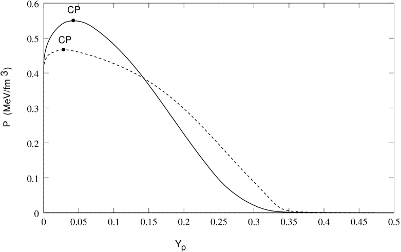
FIG. 2.: Binodal section for the QMC model (solid line) and for the NL1 (dashed line). The critical point (CP) is indicated; the liquid (gas) phase is to the right (left) of CP.

FIG. 3.: Proton density of ⁴⁰Ca in the Thomas-Fermi approximation for the QMC model (solid line) and for the NL1 (dashed line).

FIG. 4.: The droplet density surface energy as a function of the central proton fraction for the QMC model with (dashed line) and without (solid line) the electromagnetic field, and for the NL1 without the electromagnetic field (dotted line). Results for a droplet with a total of 20 particles.

FIG. 5.: The droplet density surface energy as a function of the central proton fraction for the QMC model with the electromagnetic field for a droplet with a total of 40 (solid line) and 20 (dashed line) particles.

FIG. 6.: Proton radius for a droplet with $A=20$ as a function of the central proton fraction. The meaning of the lines is the same as in Fig. 4.

FIG. 7.: Total proton fraction $Y_{tot}=N_{p}/A$ in the droplet with $A=20$ as a function of the central proton fraction. The meaning of the lines is the same as in Fig. 4.

FIG. 8.: Neutron skin thickness as a function of the central proton fraction for a droplet with $A=20$. The meaning of the lines is the same as in Fig. 4.