Analysis of the ${}^{16}O(p,\gamma)^{17}F$ capture reaction using the shell model embedded in the continuum

Abstract

We apply the realistic shell model which includes the coupling between many-particle (quasi-)bound states and the continuum of one-particle scattering states, called the Shell Model Embedded in the Continuum, to the spectroscopy of mirror nuclei: ¹⁷F and ¹⁷O, as well as to the description of low energy cross section (the astrophysical $S$ factor) for $E1$, $E2$ and $M1$ components in the capture reaction: ${}^{16}\mbox{O}(p,\gamma)^{17}\mbox{F}$. With the same microscopic input we calculate the phase shifts and differential cross-section for the elastic scattering of protons on ${}^{16}\mbox{O}$.

I Introduction

Microscopic description of weakly bound exotic nuclei close to the drip-lines such as, e.g., ${}^{8}\mbox{B}$ or ${}^{11}\mbox{Li}$ in their ground state (g.s.), or nuclei close to the $\beta$-stability line in the excited configurations like, e.g., ${}^{17}\mbox{F}$ in the first excited state $J^{\pi}=1/2^{+}$, is an exciting theoretical challenge due to the proximity of particle continuum. Closeness of the scattering continuum implies that virtual excitations to continuum states cannot be neglected as they modify the effective interactions and cause the large spatial dimension of nuclear density distribution and, in particular, the existence of halo structures. Even basic concepts of the nuclear collective model hardly apply for those weakly bound configurations as the particle motion in the weakly bound orbit is presumably decoupled from the rest of the system [1]. The microscopic description of such exotic configurations should treat properly the residual coupling of discrete configurations and the scattering continuum. Recently, it was proposed to approach this difficult problem in the quantum open system formalism which does not separate the subspaces of (quasi-) bound (the $Q$ subspace) and scattering (the $P$ subspace) states [2, 3]. Such a formalism can be provided by the Continuum Shell Model (CSM) [4] which in the restricted space of configurations generated using the finite-depth potential has been studied for the giant resonances and for the radiative capture reactions probing the microscopic structure of these resonances [4, 5, 6].

In this context, capture reaction ${}^{16}\mbox{O}(p,\gamma)^{17}\mbox{F}$ is interesting for several reasons. First of all, precise experimental data in the energy range from 200 keV to 3750 keV are now available [7] and the decays to the g.s. ($J^{\pi}=5/2^{+}$) and to the first excited state ($J^{\pi}=1/2^{+}$) of ${}^{17}\mbox{F}$ have been accurately resolved [7]. The strikingly different behavior of the astrophysical $S$-factor for the proton capture into the $5/2^{+}$ state and into the $1/2^{+}$ weakly bound state ($Q=105$ keV) has been explained by the existence of proton halo in the $1/2^{+}$ state of ${}^{17}\mbox{F}$ [7]. Different theoretical approaches, including the potential model [7, 8], the model based on the Generator Coordinate Method (GCM) [9], or the $K$- and $R$-matrix analysis [10], have been tried to describe this reaction. Moreover, an expected simplicity of the low energy wave functions in ${}^{16}\mbox{O}$, ${}^{17}\mbox{O}$ and ${}^{17}\mbox{F}$, allows to test certain salient features of models such as the effective interactions between $Q$ and $P$ subspaces and the possible quenching of matrix elements of the residual coupling which depends on the model space used in the calculations.

Secondly, the exact knowledge of rate for the reaction ${}^{16}\mbox{O}(p,\gamma)^{17}\mbox{F}$ is necessary for modelling of nucleosynthesis process in the hydrogen-burning stars. Explosive hydrogen burning is believed to occur at various sites in the Universe, including novas, X-ray bursts, or the supermassive stars [11, 12]. Hydrogen burning of second-generation stars proceeds mainly through proton - proton chain and CNO cycle. The changeover from the $pp$ chain to the CNO cycle happens near $T\simeq 2\cdot 10^{7}$K. The reaction ${}^{16}\mbox{O}(p,\gamma)^{17}\mbox{F}$ is of particular interest in this context as it provides a link to the higher branches of the CNO cycle. In particular, it starts the sidebranch : ${}^{16}\mbox{O}(p,\gamma)^{17}\mbox{F}(p,\gamma)^{18}\mbox{Ne}({\beta}^{+}\nu)^{18}\mbox{F}(p,\alpha)^{15}\mbox{O}$. The contribution of CNO cycles to the total amount of produced energy in the Sun is small and CNO neutrinos account only for about 0.02 of the total neutrino flux [13]. Moreover, most of them are coming from the decay of ${}^{13}\mbox{N}$ and ${}^{15}\mbox{O}$ in the main CNO cycle CNO-I. Flux of ’${}^{17}\mbox{F}$-neutrinos’, which is again two orders of magnitude smaller than the flux of neutrinos from ${}^{13}\mbox{N}$ and ${}^{15}\mbox{O}$ in CNO-I reactions, is controlled by the reaction ${}^{16}\mbox{O}(p,\gamma)^{17}\mbox{F}$ in the CNO-II cycle. Hence, the measurement of CNO neutrinos coming from different sources provides an accurate handle on the thermonuclear reaction process in stars like the Sun and allows in principle to distinct between different branches of the CNO cycle.

The Shell Model Embedded in the Continuum (SMEC) model, in which realistic Shell Model (SM) solutions for (quasi-)bound states are coupled to the one-particle scattering continuum, is a recent development of the Continuum Shell Model (CSM) [4, 5, 6] for the description of complicated low energy excitations of weakly bound nuclei. The SMEC approach is based on the realistic SM which is used to generate the $N$-particle wave functions. This deliberate choice implies that the coupling between SM states and the one-particle scattering continuum has to be given by the residual nucleon - nucleon interaction. In SMEC, like in the CSM, the bound (interior) states together with its environment of asymptotic scattering channels form a quantum closed system. Using the projection operator technique, one separates the $P$ subspace of asymptotic channels from the $Q$ subspace of many-body localized states which are build up by the bound single-particle (s.p.) wave functions and by the s.p. resonance wave functions. $P$ subspace is assumed to contain $(N-1)$-particle states with nucleons on bound s.p. orbits and one nucleon in the scattering state. Also the s.p. resonance wave functions outside of the cutoff radius $R_{cut}$  are included in the $P$ subspace. The resonance wave functions for $r<R_{cut}$  are included in the $Q$ subspace. The wave functions in $Q$ and $P$ are then properly renormalized in order to ensure the orthogonality of wave functions in both subspaces. The application of the SMEC model for the description of structure for mirror nuclei: ${}^{8}\mbox{B}$, ${}^{8}\mbox{Li}$, and capture cross sections for mirror reactions: ${}^{7}\mbox{Be}(p,\gamma)^{8}\mbox{B}$, ${}^{7}\mbox{Li}(n,\gamma)^{8}\mbox{Li}$ has been published recently [2, 3].

We aim in SMEC at a microscopic description of low lying, complicated many-body bound and resonance states. For that reason, the description of particle continuum is restricted to the subset of one-nucleon decay channels. This should be a reasonable approach for describing the structure of mirror nuclei ${}^{17}\mbox{F}$ and ${}^{17}\mbox{O}$ around ${}^{16}\mbox{O}$, and the capture reactions: ${}^{16}\mbox{O}(p,\gamma)^{17}\mbox{F}$ and ${}^{16}\mbox{O}(n,\gamma)^{17}\mbox{O}$. One expects that at higher excitation energies, e.g., above $\alpha$ emission threshold, the one-particle continuum approximation is too restrictive and the residual correlations generated in bound state wave functions by the coupling to those channels cannot be described. Effects of such correlations have been seen in the structure of $J^{\pi}=3^{+}$ resonances in ${}^{8}\mbox{B}$ and ${}^{8}\mbox{Li}$ [3] which strongly couples to the three-particle decay channels. In this case, one should try to employ methods based on the cluster expansion of the wave function and the three-body continuum models [14, 15, 16]. More complicated two-particle channels like, e.g., the $\alpha$ - decay channel, can be treated in SMEC, following the approach of Balashov et al. [17].

The paper is organized as follows. In Sect. II, we remind certain elements of the SMEC formalism and, in particular, those features of the $S$-matrix in SMEC which are involved in the calculation of the elastic cross-sections, phase shifts and the capture cross-sections. Sect. III is devoted to the discussion of specific properties of ${}^{17}\mbox{F}$ and ${}^{17}\mbox{O}$. In particular, properties of the matrix elements of the effective operator which couple $Q$ and $P$ subspaces in ${}^{17}\mbox{F}$ and ${}^{17}\mbox{O}$ will be discussed in Sect. III.B. Features of the self-consistent average potentials in $Q$ subspace for different many-body states of ${}^{17}\mbox{F}$ will be presented in Sect. III.C. Sect. IV is devoted to the discussion of ${}^{16}\mbox{O}(p,\gamma)^{17}\mbox{F}$ capture cross sections for different multipolarities and different final states of ${}^{17}\mbox{F}$. The differential elastic cross-section and the elastic phase-shifts in $\mbox{p}+{{}^{16}}\mbox{O}$ scattering will be compared to the experimental data in Sect. V. Summary and outlook will be given in Sect. VI.

II The formalism of Shell Model Embedded in the Continuum

The full solution of SMEC approach is constructed in three steps. In the first step, one calculates the (quasi-) bound many-body states in $Q$ subspace. For that one solves the multiconfigurational SM problem :

$$H_{QQ}{\Phi}_{i}=E_{i}{\Phi}_{i}$$ (1)

where $H_{QQ}\equiv QHQ$  is the SM effective Hamiltonian which is appropriate for the SM configuration space used. For solving (1), we use the code ANTOINE [18] which employs the Lanczos algorithm and allows for the diagonalization in large model spaces.

For the coupling between bound and scattering states around ${}^{16}\mbox{O}$, we use either a combination of Wigner and Bartlett forces (WB force) [3] :

$$V_{12}=-V_{12}^{(0)}[\alpha+(1-\alpha)P_{12}^{\sigma}]\delta({\bf r}_{1}-{\bf r}_{2})~{}\ ,$$ (2)

or the density dependent interaction (DDSM1) :

$$V_{12}=\left[{\rho}(r){\hat{v}}_{00}^{in}(1-{\rho}(r)){\hat{v}}_{00}^{ex}{\tau}_{1}{\cdot}{\tau}_{2}\left({\rho}(r){\hat{v}}_{01}^{in}+(1-{\rho}(r)){\hat{v}}_{01}^{ex}\right)\right]\delta({\bf r}_{1}-{\bf r}_{2})~{}\ .$$ (3)

$P_{12}^{\sigma}$ in (2) is the spin exchange operator and ${\rho}(r)$ in (3) is :

$${\rho}(r)=\left[1+\exp\left(\frac{r-r_{0}}{d}\right)\right]^{-1}~{}\ .$$ (4)

with $r_{0}=2.64$ fm and $d=0.58$ fm. The DDSM1 force (3) has four parameters determined as: ${\hat{v}}_{00}^{in}=36.45$, ${\hat{v}}_{00}^{ex}=-297.9$, ${\hat{v}}_{01}^{in}=109.4$ and ${\hat{v}}_{01}^{ex}=115.5$, all in units MeV$\cdot$fm³. Similar force has been used by Schwesinger and Wambach [19] for the description of giant resonances in (1$p$ - 1$h$) - (2$p$ - 2$h$) space. However, as compared to their interaction which is close to the Landau - Migdal type of interactions, the DDSM1 parameters ${\hat{v}}_{00}^{in}$, ${\hat{v}}_{00}^{ex}$, ${\hat{v}}_{01}^{in}$ and ${\hat{v}}_{01}^{ex}$, are reduced by a constant factor 0.68. Also the parameter $r_{0}$ has been somewhat reduced to better fit the experimental matter radius in oxygen. For the WB residual interaction (2), the overall strength $V_{12}^{(0)}$ is adjusted to reproduce as good as possible the energy spectra and the decay widths of states in nuclei around ${}^{16}\mbox{O}$. A reasonable compromise is provided by $V_{12}^{(0)}=300$ MeV$\cdot$fm³. The relative contribution of spin exchange term has been discussed for the $p$-shell nuclei ${}^{8}\mbox{B}$ and ${}^{8}\mbox{Li}$ [3]. It was argued that the spin exchange part is very small ($(1-\alpha)\simeq 0$) for most $p$-shell nuclei but is expected to increase for heavier nuclei. In present studies, we use $(1-\alpha)=0.27$, which is a standard value in the $1s0d$ mass region [4]. It should be stressed also that matrix elements of $H_{QQ}$ are not modified by the residual coupling between $P$ and $Q$ because they are fitted to experimental discrete levels and narrow resonances in the continuum and, therefore, they are believed to contain already those coupling effects.

The SM wave function has an incorrect asymptotic radial behavior for unbound states. Therefore, to generate both the radial s.p. wave functions in the $Q$ subspace and the scattering wave functions in $P$ subspace we use the average potential of SW type with the spin-orbit part included:

$$U(r)=V_{0}f(r)+V_{SO}{{\mathchar 22\relax\mkern-9.0mu\lambda}}_{\pi}^{2}(2{\bf l}\cdot{\bf s})\frac{1}{r}\frac{d{f}(r)}{dr}+V_{C}~{}\ ,$$ (5)

where ${{\mathchar 22\relax\mkern-9.0mu\lambda}}_{\pi}^{2}=2\,$fm² is the pion Compton wavelength and $f(r)$ is the spherically symmetrical SW formfactor :

$$f(r)=\left[1+\exp\left(\frac{r-R_{0}}{a}\right)\right]^{-1}~{}\ .$$ (6)

The Coulomb potential $V_{C}$ in (5) is calculated for the uniformly charged sphere with radius $R_{0}$.

For the continuum part, one solves the coupled channel equations:

$$(E^{(+)}-H_{PP}){\xi}_{E}^{c(+)}\equiv\sum_{c^{{}^{\prime}}}(E^{(+)}-H_{cc^{{}^{\prime}}}){\xi}_{E}^{c^{{}^{\prime}}(+)}=0~{}\ ,$$ (7)

where index $c$  denotes different channels and $H_{PP}\equiv PHP$ . The superscript $(+)$ means that boundary conditions for incoming wave in the channel $c$ and outgoing scattering waves in all channels are used. The channel states are defined by coupling of one nucleon in the scattering continuum to the many-body SM state in $(N-1)$-nucleus. The channel - channel coupling potential in (7) is :

$$H_{cc^{{}^{\prime}}}=(T+U){\delta}_{cc^{{}^{\prime}}}+{\upsilon}_{cc^{{}^{\prime}}}^{J}~{}\ ,$$ (8)

where $T$ is the kinetic-energy operator and ${\upsilon}_{cc^{{}^{\prime}}}^{J}$ is the channel-channel coupling generated by the residual interaction. The potential for channel $c$ in (8) consists of ’initial guess’, $U(r)$, and diagonal part of coupling potential ${\upsilon}_{cc}^{J}$ which depends on both the s.p. orbit ${\phi}_{l,j}$ and the considered many-body state $J^{\pi}$. This modification of the initial potential $U(r)$ change the generated s.p. wave functions ${\phi}_{l,j}$ defining $Q$ subspace which in turn modify the diagonal part of the residual force, etc. This means that the solution of coupled channel equations (7) is accompanied by the self-consistent iterative procedure which yields for each channel independently the new self-consistent potential :

$$U^{(sc)}(r)=U(r)+{\upsilon}_{cc}^{J(sc)}(r)~{}\ ,$$ (9)

and consistent with it the new renormalized matrix elements of the coupling force. The parameters of the initial potential $U(r)$ are chosen in such a way that $U^{(sc)}(r)$ reproduces energies of experimental s.p. states, whenever their identification is possible.

The third system of equations in SMEC consists of inhomogeneous coupled channel equations:

$$(E^{(+)}-H_{PP}){\omega}_{i}^{(+)}=H_{PQ}{\Phi}_{i}\equiv w_{i}$$ (10)

with the source term $w_{i}$ which is primarily given by the structure of $N$ - particle SM wave function ${\Phi}_{i}$ . The explicit form of this source is given in [3]. These equations define functions ${\omega}_{i}^{(+)}$ , which describe the decay of quasi-bound state ${\Phi}_{i}$  in the continuum. The source $w_{i}$  couples the wave function of $N$-nucleon localized states with $(N-1)$-nucleon localized states plus one nucleon in the continuum. Formfactor of the source term is given by the self-consistently determined s.p. wave functions.

The full solution of SMEC equations is expressed by three functions: ${\Phi}_{i}$ , ${\xi}_{E}^{c}$  and ${\omega}_{i}$ [3, 4] :

$${\Psi}_{E}^{c}={\xi}_{E}^{c}+\sum_{i,j}({\Phi}_{i}+{\omega}_{i})\frac{1}{E-H_{QQ}^{eff}}<{\Phi}_{j}\mid H_{QP}\mid{\xi}_{E}^{c}>~{}\ ,$$ (11)

where

$$H_{QQ}^{eff}=H_{QQ}+H_{QP}G_{P}^{(+)}H_{PQ}~{}\ ,$$ (12)

is the effective SM Hamiltonian which includes the coupling to the continuum, and $G_{P}^{(+)}$  is the Green function for the motion of s.p. in the $P$ subspace. Matrix $H_{QQ}^{eff}$ is non-Hermitian (the complex, symmetric matrix) for energies above the particle emission threshold and Hermitian (real) for lower energies. The eigenvalues ${\tilde{E_{i}}}-\frac{1}{2}i{\tilde{{\Gamma}_{i}}}$ are complex for decaying states and depend on the energy $E$ of particle in the continuum. The energy and width of resonance states are determined by the condition: $\tilde{E_{i}}(E)=E$ [4]. The eigenstates corresponding to these eigenvalues can be obtained by the orthogonal but in general non-unitary transformation :

$${\tilde{\Phi}}_{i}=\sum_{j}\beta_{ij}{\Phi}_{j}$$ (13)

where the coefficients $\beta_{ij}$ form a complex matrix of eigenvectors in the SM basis satisfying :

$$\sum_{k}\beta_{ik}\beta_{jk}=\delta_{ij}$$ (14)

Analogously, one can define :

$${\tilde{\omega}}_{i}=\sum_{j}\beta_{ij}\omega_{j}$$ (15)

and

$${\tilde{\Omega}}_{i}={\tilde{\Phi}}_{i}+{\tilde{\omega}}_{i}~{}\ .$$ (16)

Inserting them in (11), one obtains :

$${\Psi}_{E}^{c}={\xi}_{E}^{c}+\sum_{i}{\tilde{\Omega}_{i}}\frac{1}{E-{\tilde{E}_{i}}+(i/2){\tilde{\Gamma}_{i}}}<{\tilde{\Phi}_{i}}\mid H_{QP}\mid{\xi}_{E}^{c}>$$ (17)

for the continuum many-body wave function projected on channel $c$, where

$${\tilde{\Omega}_{i}}={\tilde{\Phi}_{i}}+\sum_{c}\int_{{\varepsilon}_{c}}^{\infty}dE^{{}^{\prime}}{\xi}_{E^{{}^{\prime}}}^{c}\frac{1}{E^{(+)}-E^{{}^{\prime}}}<{\xi}_{E^{{}^{\prime}}}^{c}\mid H_{PQ}\mid{\tilde{\Phi}_{i}}>~{}\ ,$$ (18)

is the wave function of discrete state modified by the coupling to the continuum states. It should be stressed that the SMEC formalism is fully symmetric in treating the continuum and bound state parts of the solution : ${\Psi}_{E}^{c}$ represents the continuum state modified by the discrete states, and ${\tilde{\Omega}_{i}}$ represents the discrete state modified by the coupling to the continuum.

A Radiative capture and electromagnetic transitions

Having obtained the full solution of SMEC, one can calculate many observable quantities. E.g., the calculation of capture cross-section goes as follows. The initial SMEC wave function for the $[\mbox{p}\bigotimes(N-1)]^{J_{i}^{{\pi}_{i}}}$ system is :

$$\Psi_{i}(r)=\sum_{l_{a}j_{a}}i^{l_{a}}{\psi_{l_{a}j_{a}}^{J_{i}}(r)\over r}\biggl{[}\bigl{[}Y^{l_{a}}\times\chi^{s}\bigr{]}^{j_{a}}\times\chi^{I_{t}}\biggr{]}^{(J_{i})}_{m_{i}}~{}~{}~{}\ ,$$ (19)

and the final SMEC wave function for the $N$-system in the many-body state $J_{f}^{{\pi}_{f}}$ is :

$$\Psi_{f}(r)=\sum_{l_{b}j_{b}}A_{l_{b}sj_{b}}^{j_{b}I_{b}J_{f}}{u_{l_{b}j_{b}}^{J_{f}}(r)\over r}\biggl{[}\bigl{[}Y^{l_{b}}\times\chi^{s}\bigr{]}^{j_{b}}\times\chi^{I_{t}}\biggr{]}^{(J_{f})}_{m_{f}}\ .$$ (20)

$I_{t}$  and $s$  denote the spin of target nucleus and incoming proton, respectively. $A_{l_{b}sj_{b}}^{j_{b}I_{b}J_{f}}$  is the coefficient of fractional parentage and $u_{l_{b}j_{b}}^{J_{f}}$  is the s.p. wave in the many-particle state $J_{f}$ . These SMEC wave functions (19,20) are then used to calculate the transition amplitudes $T^{E{\cal L}}$ and $T^{M1}$ for $E1$ , $E2$  and $M1$ transitions, respectively [2, 3]. The radiative capture cross section is :

$$\sigma^{E1,M1}={16\pi\over 9}\biggl{(}{k_{\gamma}\over k_{p}}\biggr{)}^{3}\biggl{(}{\mu\over\hbar c}\biggr{)}\biggl{(}{e^{2}\over\hbar c}\biggr{)}{1\over 2s+1}~{}{1\over 2I_{t}+1}\sum\mid T^{E1,M1}\mid^{2}$$ (21)

$$\sigma^{E2}={4\pi\over 75}\biggl{(}{k_{\gamma}^{5}\over k_{p}^{3}}\biggr{)}\biggl{(}{\mu\over\hbar c}\biggr{)}\biggl{(}{e^{2}\over\hbar c}\biggr{)}{1\over 2s+1}~{}{1\over 2I_{t}+1}\sum\mid T^{E2}\mid^{2}$$ (22)

and $\mu$  stands for the reduced mass of the system.

Another interesting quantities are $B(E\lambda)$, $B(M\lambda)$ transition matrix elements between the SMEC wave functions $J_{i}^{{\pi}_{i}}$ and $J_{f}^{{\pi}_{f}}$ for the [$N$] - system :

$$B(\Pi\lambda;J_{i}^{\pi_{i}}\rightarrow J_{f}^{\pi_{f}})=\frac{\mid<\Psi_{f}(J_{f}^{{\pi}_{f}})||{\hat{O}}(\Pi\lambda)||\Psi_{i}(J_{i}^{{\pi}_{i}})>{\mid}^{2}}{2J_{i}+1}~{}~{}~{}\ ,$$ (23)

where $\Pi\,=\,$ E (electric) or M (magnetic), and $\lambda\,=\,1,2...$ (multipolarity). ${\hat{O}}(\Pi\lambda)$ in (23) is the electromagnetic transition operator [20].

B Properties of the $S$-matrix

The $S$-matrix for the scattering of a nucleon by a nucleus is given by the asymptotic behavior of the total wave function (17) :

$${\Psi}_{c}^{(c_{0})}={\xi}_{c}^{(c_{0})}+\sum_{i}{\tilde{\Omega}_{i}}\frac{1}{E-{\tilde{E}_{i}}+(i/2){\tilde{\Gamma}_{i}}}<{\tilde{\Phi}_{i}}\mid H\mid{\xi}_{c}^{(c_{0})}>$$ (24)

with the incoming wave only in the channel $c_{0}$. The asymptotic conditions for the solution (24) have been analyzed in Ref. [4]. Here we only give the final result for the amplitude of the partial width :

$${\gamma}_{c}^{(n)}=-\exp(-i{\delta}_{c}^{(0)})\left(\frac{4m_{r}}{{\hbar}^{2}k_{c}}\right)^{1/2}\sum_{i}{\beta}_{ni}\sum_{c^{{}^{\prime}}}\int dr{\xi}_{c^{{}^{\prime}}}^{(c)}(r)w_{c^{{}^{\prime}}}^{(i)}(r)~{}~{}~{}\ ,$$ (25)

where ${\delta}_{c}^{(0)}$ is the background scattering phase :

$${\delta}_{c}^{(0)}=\frac{1}{2}\mbox{arg}S_{cc}^{(0)}~{}\ ,$$ (26)

and $S_{cc}^{(0)}$ is determined from the asymptotic, large distance behavior of ${\xi}_{c}^{(c)}$. Using the proportionality relation between matrix elements in (24) and the amplitudes of partial width (25), one derives the $S$-matrix elements :

$$S_{cc_{0}}=S_{cc_{0}}^{(0)}-i\exp[i({\delta}_{c}^{(0)}+{\delta}_{c_{0}}^{(0)})]\sum_{n}\frac{{\gamma}_{c}^{(n)}{\gamma}_{c_{0}}^{(n)}}{E-{\tilde{E}}_{n}+\frac{1}{2}i{\tilde{\Gamma}}_{n}}~{}~{}~{}\ .$$ (27)

Amplitudes of the partial widths ${\gamma}_{c}^{(n)}$ as well as the real ${\tilde{E}}_{n}$ and imaginary ${\tilde{\Gamma}}_{n}$ parts of complex eigenvalues of the effective shell model Hamiltonian $H_{QQ}^{eff}$ (12) entering the $S$-matrix elements are explicitly energy dependent. ${\gamma}_{c}^{(n)}$ are also complex due to the channel - channel coupling and the mixing of quasi-bound states embedded in the continuum [4]. The partial width for channel $c$ can then be defined by :

$${\Gamma}_{n,c}={\mid}{\gamma}_{c}^{(n)}{\mid}^{2}~{}~{}~{}\ ,$$ (28)

though the total width ${\Gamma}_{n}$ is no longer sum of partial widths [21] :

$$\sum_{c}{\mid}{\gamma}_{c}^{(n)}{\mid}^{2}={\tilde{\Gamma}}_{n}\sum_{i}{\mid}{\beta}_{ni}{\mid}^{2}\geq{\tilde{\Gamma}}_{n}$$ (29)

because the eigenvectors $\beta_{ni}$ are normalized in a sense of (14), what implies :

$$\sum_{i}\mid\beta_{ni}{\mid}^{2}\geq 1~{}\ .$$ (30)

III Spectroscopy of ${}^{17}\mbox{F}$ and ${}^{17}\mbox{O}$ nuclei

A The effective interactions for the $0p1s1d$ SM space

For the purpose of the present study we have constructed SM effective interactions in the cross-shell model space connecting the $0p$ and $1s0d$ shells. The interactions have three distinctive parts: the $0p$-shell part taken to be the CK(8-16) interaction [22], the $1s0d$-shell part taken to be the Brown–Wildenthal interaction [23]. For the cross-shell matrix elements, we use the G matrix of Kahana, Lee and Scott (KLS) [24]. This part of the interaction has to be modified phenomenologically. We proceed as follow: the $1s0d$ s.p. energies above the ⁴He core are taken from generalized monopoles fit of energies of single-particle and single-hole states over the mass table [25]. Then the cross monopoles are adjusted to reproduce ¹⁵N, ¹⁵O and ¹⁷O, ¹⁷F spectra. The center of mass components are removed with the usual Gloeckner - Lawson prescription [26] adding a center of mass kinetic energy hamiltonian. For natural parity states, we consider only 0$\hbar\omega$ excitations and for non natural parity states, 1$\hbar\omega$ excitations. Of course, it is well known and has been studied in the past, that ¹⁶O (and¹⁷O, ¹⁷F) have significant amount of $2p-2h$ ($3p-2h$) and $4p-4h$ ($5p-4h$) admixtures in their low lying states [27, 28]. Nevertheless, the shell model calculation of these admixtures is not straightforward:

• Firstly, it has been already stressed in the past by different authors [29, 30, 31], that $N\hbar\omega$ mixing converges slowly with $N$ and, if stopped for example after $N=2$, causes a strong lowering of $0p-0h$ states due to 2$\hbar\omega$ pairing correlations which were already present in pure $2p-2h$ states. One could overpass this artifact of the calculation by artificially lowering the $N\hbar\omega$ unperturbed configurations through the monopoles of the interaction, but the control of convergence of the mixing would be impossible as higher order admixtures would destroy the picture.

• Secondly, the building blocks of our interaction are made of 0$\hbar\omega$ $0p$ and $1s0d$ phenomenological interactions, which in principle already contain, in particular through pairing renormalizations, the higher order correlations. For this reason, we have decided to fix the unperturbed ($4p-4h$) 0⁺ state around its experimental energy (6.049 MeV).

Again, the derivation of precise correlated wave functions for ¹⁶O and ¹⁷O, ¹⁷F is out of the scope of this paper and we will refer to the mixing derived by other studies [27, 28].

B The effective operator of the residual coupling

Expressions for the matrix elements of residual interaction which couples $P$ and $Q$ subspaces have been given in Refs. [4, 3]. There are two kinds of coupling operators. The channel - channel coupling reduced matrix elements involve one-body operators :

$${\cal O}^{K}_{{\beta}{\delta}}=(a^{\dagger}_{\beta}{\tilde{a}}_{\delta})^{K}$$ (31)

Diagonal part of ${\cal O}$ induce the renormalization of the s.p. average potential. Matrix elements of the operators ${\cal O}$ are calculated between different many-body states in the $(N-1)$-system, i.e., in ${}^{16}\mbox{O}$, and they depend sensibly on the amount of $2p-2h$ and $4p-4h$ correlations in the g.s. of ${}^{16}\mbox{O}$.

Reduced matrix elements of the source term $w_{i}$ in the inhomogeneous coupled channel equations (10) contain a product of two annihilation operators and one creation operator :

$${\cal R}^{j_{\alpha}}_{{\gamma}{\delta}(L){\beta}}=(a^{\dagger}_{\beta}({\tilde{a}}_{\gamma}{\tilde{a}}_{\delta})^{L})^{j_{\alpha}}~{}~{}~{}~{}\ .$$ (32)

Operators ${\cal R}$ enter in the calculation of complex eigenvalues of $H_{QQ}^{eff}$. Matrix elements of ${\cal R}$ are calculated between different initial state wave functions in either [$\mbox{p}\bigotimes(N-1)$] or [$\mbox{n}\bigotimes(N-1)$] system, i.e., in ${}^{17}\mbox{F}$ or ${}^{17}\mbox{O}$, and a given final state wave function in ${}^{16}\mbox{O}$. These matrix elements depend on the configuration mixing in the many-body wave functions of ${}^{17}\mbox{F}$, ${}^{17}\mbox{O}$ and ${}^{16}\mbox{O}$.

We perform the SM calculations for ${}^{16}\mbox{O}$ ground state in which admixture of $2p-2h$ and $4p-4h$ configurations are neglected :

$$|^{16}\mbox{O},0_{1}^{+}> = a_{00}{|(0p-0h)^{J=0}>}+a_{22}{|(2p-2h)^{J=0}>}+a_{44}{|(4p-4h)^{J=0}>}+\cdots$$ (33)

$$\simeq a_{00}{|(0p-0h)^{J=0}>}$$ (34)

i.e., the g.s. of ${}^{16}\mbox{O}$ is taken to be a pure $(0p^{12})$ $0p-0h$ configuration and the second excited $0_{2}^{+}$ state with predominantly $4p-4h$ structure is not mixed with the ground state. How big are these $\mbox{n}p-\mbox{n}h$ admixture depends on the SM effective interaction and the effective s.p. space used [27, 28]. In Table I we give results of different SM calculations for $0_{1}^{+}$ in ${}^{16}\mbox{O}$.

Likewise in ${}^{17}\mbox{O}$ and ${}^{17}\mbox{F}$, the g.s. $J^{\pi}=5/2_{1}^{+}$ and the excited states $J^{\pi}=1/2_{1}^{+}$, $3/2_{1}^{+}$ correspond in our approximation to the pure configuration of one particle in, respectively, $0d_{5/2}$, $1s_{1/2}$ or $0d_{3/2}$ shells outside of the $(0p^{12})$-core of ${}^{16}\mbox{O}$, i.e.:

$$|^{17}\mbox{F};J^{\pi},{\pi=+}> = a_{10}^{J^{\pi}}{|(1p-0h)^{J^{\pi}}>}+a_{32}^{J^{\pi}}{|(3p-2h)^{J^{\pi}}>}+\cdots$$ (35)

$$\simeq a_{10}^{J^{\pi}}{|(1p-0h)^{J^{\pi}}>}~{}\ .$$ (36)

The amount of these admixture calculated by Brown–Green [27] and Zuker–Buck–McGrory [28] can be read from the Table II. The experimental spectroscopic amplitudes for $5/2_{1}^{+}$ and $1/2_{1}^{+}$ states can be found in Table III.

The negative parity states involve the excitations across the shell closure and involve one hole in the $p$ shell and two particles in the $1s0d$ shells. In our model of ${}^{16}\mbox{O}$ where $2p-2h$ and $4p-4h$ configurations are neglected, the spectroscopic factors of negative parity SM states are equal zero. Hence the particle decay width for these states is coming from the functions $\omega_{i}$ (10) which describe the continuation of $Q$ space wave functions $\Phi_{i}$ into $P$, i.e., from the modification of discrete states by the coupling to the continuum (18).

Neglecting higher order correlations in the g.s. of ${}^{16}\mbox{O}$ and in positive parity excited states of either ${}^{17}\mbox{F}$ or ${}^{17}\mbox{O}$ means that residual coupling between $Q$ and $P$ which involves those states should be properly rescaled, i.e., the matrix elements of $\cal{O}$, $\cal{R}$ should be quenched :

$$<{{}^{16}\mbox{O}},J_{f}|{\cal O}|{{}^{16}\mbox{O}},J_{i}>^{(quenched)}=(a_{00})^{2}<{{}^{16}\mbox{O}},J_{f}|{\cal O}|{{}^{16}\mbox{O}},J_{i}>^{(non-quenched)}$$ (37)

$$<{{}^{16}\mbox{O}},J_{f}|{\cal R}|{{}^{17}\mbox{O}},J_{i}>^{(quenched)}=a_{00}a_{10}^{J_{i}}<{{}^{16}\mbox{O}},J_{f}|{\cal R}|{{}^{17}\mbox{O}},J_{i}>^{(non-quenched)}$$ (38)

$$<{{}^{16}\mbox{O}},J_{f}|{\cal R}|{{}^{17}\mbox{F}},J_{i}>^{(quenched)}=a_{00}a_{10}^{J_{i}}<{{}^{16}\mbox{O}},J_{f}|{\cal R}|{{}^{17}\mbox{F}},J_{i}>^{(non-quenched)}$$ (39)

Amount of configuration mixing for negative parity states is large (two particles in $1s0d$ shell and 1 hole in $0p$ shell) and therefore matrix elements of ${\cal R}$ are not quenched. In our calculations, we take the values given by Brown - Green [27] for the amplitudes $a_{00}$ and $a_{10}^{J_{i}}$ (see Tables I and II).

C The self-consistent average potentials

Construction of the $Q$ subspace in SMEC is achieved by the self-consistent, iterative procedure which for a given initial average s.p. potential (5) and for a given residual two-body interaction between $Q$ and $P$ yields the self-consistent s.p. potential $U^{(sc)}(r)$ which depends on the s.p. wave function ${\phi}_{l,j}$, the total spin $J$ of the $N$-nucleon system as well as on the one-body matrix elements of $(N-1)$ - nucleon daughter system. As explained above, the positive parity states in ${}^{17}\mbox{F}$ and ${}^{17}\mbox{O}$ are described as a pure one particle configuration in $1s0d$ shells. Consequently, the spectroscopic factors for the states $J^{\pi}={1/2}^{+}~{},{5/2}^{+}~{}$ and ${3/2}^{+}~{}$ are equal 1. Consistently with this approximation, we can identify position of proton (neutron) s.p. orbits $1s_{1/2}$, $0d_{5/2}$ and $0d_{3/2}$ with, respectively, $J^{\pi}={1/2}^{+}$, ${5/2}^{+}~{}$ and ${3/2}^{+}~{}$ many body states of ${}^{17}\mbox{F}$ (${}^{17}\mbox{O}$), i.e., we may ask that $U^{(sc)}(J^{\pi})$ provides the energy of s.p. orbit at the energy of the corresponding many-body state with respect to the threshold. This choice is essential for quantitative description of radiative capture cross-section. Consequently, the initial SW potentials $U(J^{\pi}$) have all different depth parameters. Moreover, they depend on the choice of the residual interaction coupling $P$ and $Q$. On the contrary, we keep a common radius $R_{0}=3.214\,$fm, a common diffuseness $a=0.58\,$fm and a common spin-orbit strength $V_{SO}=3.683\,$MeV for all of them. The depth parameters of initial SW potentials for [$\mbox{p}\bigotimes{}^{16}\mbox{O}$] and [$\mbox{n}\bigotimes{}^{16}\mbox{O}$] systems, are summarized in Table IV. For a given nucleus (${}^{17}\mbox{F}$ or ${}^{17}\mbox{O}$), all those different central potentials correspond to the one and the same equivalent potential $U^{(eq)}(r)$ in the SW form which binds s.p. orbits at the same energy as obtained in the self-consistent potentials for neutrons and protons. For both WB and DDSM1 residual interactions, the depth of $U^{(eq)}$ is $V_{0}=-52.46\,$MeV in ${}^{17}\mbox{F}$ and $V_{0}=-52.49\,$MeV in ${}^{17}\mbox{O}$. The potential radius, the diffuseness and the spin-orbit strength are the same as used for the initial potentials $U(J^{\pi})$. The spectrum of single-particle (-hole) energies in this potential is given in Table V for ${}^{17}\mbox{F}$ and in Table VI for ${}^{17}\mbox{O}$. These energies are determined from the data of ${}^{17}\mbox{F}$, ${}^{17}\mbox{O}$ (for particles) and ${}^{15}\mbox{N}$, ${}^{15}\mbox{O}$ (for holes). The difference of s.p. energies ${\epsilon}_{p}(1s_{1/2})-{\epsilon}_{p}(0d_{5/2})=0.495\,$MeV in ${}^{17}\mbox{F}$ and ${\epsilon}_{n}(1s_{1/2})-{\epsilon}_{n}(0d_{5/2})=0.871\,$MeV, which should be compared with the excitation energy of $J^{\pi}=1/2_{1}^{+}$ state in those nuclei, is a manifestation of the Thomas-Ehrman shift [38] and is included effectively in our equivalent and self-consistent s.p. potentials for all studied channels.

In Fig. 1 we show examples of calculated potentials in ${}^{17}\mbox{F}$ for the proton s.p. orbitals $1s_{1/2}$ and $0d_{5/2}$ in the total spin states: $J^{\pi}=1/2^{+}$ and $J^{\pi}=5/2^{+}$, respectively. The calculations have been performed using the appropriate initial potentials $U(J^{\pi})$ (see Table IV) for the DDSM1 residual interaction (3). For example, potential $U(5/2^{+})$ is chosen in such a way that the self-consistent potential $U^{(sc)}(5/2^{+})$ (see Table V) yields $0d_{5/2}$ proton s.p. orbit bound at the experimental binding energy of the ground state (g.s.) $J^{\pi}={5/2}_{1}^{+}$. Similarly, the choice of $U(1/2^{+})$ and the determination of $U^{(sc)}(1/2^{+})$ is associated with the reproduction of the experimental binding energy of the first excited state $J^{\pi}={1/2}_{1}^{+}$. The $J^{\pi}$-independent equivalent potential yields the $0d_{5/2}$ and $1s_{1/2}$ proton s.p. orbits at the position given for them in the corresponding $U^{(sc)}(5/2^{+})$ and $U^{(sc)}(1/2^{+})$ potentials.

The self-consistent potential (the solid line) strongly deviates from the SW form. In the center $U^{(sc)}(r)$ has a strong maximum which is absent in the initial potential $U(r)$ (the dashed line). The self-consistent potentials $U^{(sc)}(1/2^{+})$ and $U^{(sc)}(5/2^{+})$ are different (compare the solid curves on l.h.s.  and r.h.s. of Fig. 1), in spite of the fact that up to spin–orbit coupling the equivalent potential $U^{(eq)}$ (the dotted lines) in these states is identical. This clearly shows how strong is the state dependence of both the self-consistent average fields and the renormalized matrix elements of the coupling force. One should also notice the difference in surface region between $U^{(sc)}(1/2^{+})$, $U^{(sc)}(5/2^{+})$ and $U^{(eq)}$. In $U^{(sc)}(5/2^{+})$ one may notice decrease of the potential radius in comparison with the radius of $U^{(eq)}$. However, as compared to the initial average potentials $U(5/2^{+})$ and $U(1/2^{+})$, both the self-consistent potentials $U^{(sc)}(5/2^{+})$, $U^{(sc)}(1/2^{+})$, and the equivalent potential $U^{(eq)}$ are deeper and their effective radii are bigger.

In Fig. 2 we show examples of calculated potentials in ${}^{17}\mbox{F}$ for the proton s.p. orbital $0p_{1/2}$ in the many-body states $J^{\pi}=1/2^{-}$. The calculations have been performed using the initial potentials $U(1/2^{-})$ for the WB (l.h.s. of the plot) and DDSM1 (r.h.s. of the plot) residual interactions. For both interactions, the equivalent potential $U^{(eq)}(r)$ is the same. It is interesting to notice how different are the self-consistent $U^{(sc)}(r)$ potentials for the two considered residual interactions. As a rule, the renormalization of initial s.p. potential is weaker for the density-dependent DDSM1 interaction. Similarly as for the self-consistent potentials in $J^{\pi}={5/2}^{+}$ and $J^{\pi}={1/2}^{+}$ states (see Fig. 1 ), the effective radius of $U^{(sc)}(r)$ shrinks as compared to the radius of $U^{(eq)}(r)$ . Again this effect is stronger for the WB residual interaction.

In general, the surface region of average potential shows weak sensitivity to the self-consistent correction. In our case, the radial dependence of self-consistent correction for all positive parity states in ${}^{17}\mbox{F}$ and ${}^{17}\mbox{O}$ is given by the $0p_{1/2}$ and $0p_{3/2}$ radial formfactors corresponding to the well bound single-hole state and not by the weakly bound single-particle states $1s_{1/2}$ or $0d_{5/2}$. For that reason, even for the $J^{\pi}={1/2}_{1}^{+}$ state in ${}^{17}\mbox{F}$ which is bound by 105 keV, induced renormalization of the surface in the self-consistent potential decreases the radius of potential in the surface region.

D Discussion

In this section, we shall present the SMEC results for the spectrum of mirror nuclei: ${}^{17}\mbox{F}$ and ${}^{17}\mbox{O}$. The results depend mainly on: (i) the nucleon - nucleon interaction in $Q$ subspace, (ii) the residual coupling of $Q$ and $P$ subspaces, (iii) the self-consistent average s.p. potential which generates the radial formfactor for s.p. bound wave functions and s.p. resonances, and (iv) the cutoff radius for s.p. resonances. Below, we shall comment on their relative importance.

1 Spectrum of ${}^{17}\mbox{F}$

Fig. 3 compares the SM energy spectrum of ${}^{17}\mbox{F}$ for positive parity (l.h.s. of the plot) and negative parity (r.h.s. of the plot) states, with those obtained in the SMEC approach for WB and DDSM1 residual interactions. The experimental data are plotted separately for positive and negative parity states as well. SM calculation is performed using the effective interaction described in Sect. III.A. In the column denoted ’SMEC (WB)’ we show results of SMEC approach with the residual coupling between $Q$ and $P$ subspaces which is given by the mixture of Wigner and Bartlett forces (2) with the spin-exchange parameter $(1-\alpha)=0.27$. The overall strength parameter $V_{12}^{(0)}=300\,$MeV$\cdot$fm³ has been obtained by fitting the spectra of ${}^{17}\mbox{F}$ and ${}^{17}\mbox{O}$. In the column denoted ’SMEC (DDSM1)’, the DDSM1 density dependent residual interaction (3) is used. Only the coupling matrix elements between the $J^{\pi}=0_{1}^{+}$ g.s. wave function of ${}^{16}\mbox{O}$ and all considered states in ${}^{17}\mbox{F}$ are included. Zero of the energy scale for ${}^{17}\mbox{F}$ is fixed at the experimental position of $J^{\pi}=1/2_{1}^{+}$ first excited state with respect to the proton emission threshold for all different examples of SMEC calculations which are shown in Figs. 3 and 4.

The iterative procedure to correct $U(r)$ and to include the diagonal part contribution of residual interaction has been described in the previous section. The self-consistently determined s.p. potential $U^{(sc)}(r)$ is then used to calculate radial formfactors of coupling matrix elements and s.p.  wave functions. Different initial potentials $U(J^{\pi})$ (see Table IV) are used for the calculation of self-consistent average potentials for different many-body states in ${}^{17}\mbox{F}$. These different self-consistent potentials correspond to a unique equivalent SW potential $U^{(eq)}(r)$. The renormalization of initial potential by the residual coupling of $Q$ and $P$ subspaces is the same for all states $J^{\pi}$ of the same spin and parity. For positive parity states, as a result of the restriction in SM calculations in $Q$ subspace, the renormalization of average potential operates only for s.p. orbits which have the same spin $j$ and parity $\pi$ as those of the many body states $J,\pi$. E.g., for the many body state $J^{\pi}=5/2^{+}$ of ${}^{17}\mbox{F}$ (${}^{17}\mbox{O}$), only potential of the $0d_{5/2}$ s.p. orbit is modified by the coupling to the continuum. Similarly for $J^{\pi}=1/2^{+}$ many body state and the s.p. orbit $1s_{1/2}$. For those s.p. orbits which in a given many body state are not modified by the selfconsistent renormalization, we calculate radial formfactors using the ’universal’ equivalent s.p. potential $U^{(eq)}(r)$ which does not depend neither on the many body state nor on the s.p. orbit. Of course, this special property is only due to a simple structure of ${}^{16}\mbox{O}$ and ${}^{17}\mbox{F}$ nuclei in our SM calculations. For neutrons in ${}^{17}\mbox{F}$ there is no renormalization of the average potential and we use the equivalent potential for neutrons to get the radial formfactors (see Table V). Supplementary informations concerning the results shown in Fig. 3 can be found in Table VII.

The spectrum of ${}^{17}\mbox{F}$ is insensitive to certain approximations in the SMEC. G.s. energy relative to the proton emission threshold is reasonably well reproduced by the SMEC. Coupling to the continuum induces strong relative shifts of $5/2_{1}^{+}$ and $3/2_{1}^{+}$ states with respect to the $1/2_{1}^{+}$ state and the negative parity states. The position of g.s. with respect to the energy threshold for proton emission changes by about 500 keV due to the inclusion of coupling to the g.s. of ${}^{16}\mbox{O}$ (compare columns denoted ’SM’ with those denoted ’SMEC (WB)’ and ’SMEC (DDSM1)’ in Fig. 3 and in Table VII). These shifts are generally smaller for the DDSM1 residual coupling. The coupling to excited $0_{2}^{+}$ state at $E^{*}=6.049\,$MeV in ${}^{16}\mbox{O}$ ($0_{2}^{+}$ has predominantly $4p-4h$ structure with respect to the dominant $0p-0h$ configuration in the g.s. $0_{1}^{+}$ ) is expected to be unimportant in ${}^{17}\mbox{F}$ or ${}^{17}\mbox{O}$. Calculated width of states depends on chosen residual couplings (compare ’SMEC (WB)’ with ’SMEC (DDSM1)’) and in general the agreement is better for the density dependent interaction. The effective quenching of the coupling matrix elements (37–39) for positive parity states does not solve this problem completely. To get a better agreement with the data, the energy separation of $5/2_{1}^{+}$ and $1/2_{1}^{+}$ SM states should be decreased while the splitting of $5/2_{1}^{+}$ and $3/2_{1}^{+}$ SM states should remain unchanged. This means that the separation of $1s$ subshell and the centroid od $0d$ subshells should be increased by few hundred keV. We did not however pursue the studies in this direction and we keep standard values of s.p. energies [25].

The effect of quenching of the coupling operator between $Q$ and $P$ can be seen in Fig. 4 where the comparison between the SMEC calculations with the quenching factors (entry ’SMEC (DDSM1)’) and those without quenching factors (entry ’SMEC (DDSM1^∗’) are shown. The strong downshift due to the continuum coupling is seen for the ($5/2_{1}^{+}$ - $3/2_{1}^{+}$) - pair with respect to both the negative parity states and the $1/2_{1}^{+}$ state which moves downwards much less. The effect of quenching of the coupling operator on negative parity states is, as expected, very weak.

A useful measure of the radial wave function is the $B(E2)$ transition matrix element between $1/2_{1}^{+}$ and $5/2_{1}^{+}$ bound states. In SMEC, we obtain 70.3 e²fm⁴ for DDSM1 residual coupling. This value has been calculated using the effective charges : $e_{p}=1.41$ and $e_{n}=0.47$ and the BG quenching factors (Table II). The experimental value for this transition is $B(E2)_{exp}=64.92\,$e²fm⁴. The SM prediction for this transition is $B(E2)_{SM}=32.7\,$e²fm⁴ assuming the oscillator length $b=A^{1/6}\,$fm and the same effective charges as used in the SMEC calculations. The better agreement of calculated in SMEC $B(E2)$ values with the data is mainly due to more realistic radial dependence of the $1s_{1/2}$ s.p. orbit in $J^{\pi}=1/2_{1}^{+}$ many body state. The rms radius for this orbit in SMEC is ${<r^{2}>}^{1/2}=5.212\,$fm, as compared to the value of ${<r^{2}>}^{1/2}=3.629\,$fm for the $0d_{5/2}$ s.p. orbit in $J_{1}^{\pi}=5/2^{+}$ state. Nuclear rms radius of ¹⁷F is 2.664 fm in the g.s. and 2.814 fm in the first excited state $1/2^{+}$.

2 Spectrum of ${}^{17}\mbox{O}$

Fig. 5 compares the SM energy spectrum of ${}^{17}\mbox{O}$ for positive parity (l.h.s. of the plot) and negative parity (r.h.s. of the plot) states, with those obtained in the SMEC approach for WB and DDSM1 residual interactions. The experimental data are plotted separately for positive and negative parity states as well. SM calculation is performed using the same effective interaction as used for ${}^{17}\mbox{F}$ spectrum shown in Figs. 3 and 4. In the column denoted ’SMEC (WB)’ we show results of SMEC approach with the residual coupling given by the mixture of Wigner and Bartlett forces (2). In the column denoted ’SMEC (DDSM1)’, the density dependent interaction DDSM1 is used as the residual interaction. Parameters of the residual couplings are the same as used to describe the ${}^{17}\mbox{F}$ spectrum. Only the coupling matrix elements between the $J^{\pi}=0_{1}^{+}$ g.s. wave function of ${}^{16}\mbox{O}$ and all considered states in ${}^{17}\mbox{O}$ are included. For all different examples of SMEC calculations which are shown in Fig. 5, zero on the energy scale is fixed at the experimental position of $J^{\pi}=5/2_{1}^{-}$ state which is close to the neutron emission threshold.

The self-consistently determined s.p. potential $U^{(sc)}(r)$ is then used to calculate radial formfactors of coupling matrix elements and s.p.  wave functions. Different initial potentials $U(J^{\pi})$ for [n $\bigotimes$ ¹⁶O] (see Table IV) are used for the calculation of self-consistent average potentials for different many-body states in ${}^{17}\mbox{O}$. These different self-consistent potentials correspond to a unique equivalent SW potential $U^{(eq)}(r)$ (see Table VI). For protons there is no correction from the residual interaction modifying the average potential and we use the equivalent potential for protons to get the radial formfactors (see Table VI).

The energy intervals between the g.s. and the positive parity states $1/2_{1}^{+}$ and $3/2_{1}^{+}$ in SMEC(DDSM1) calculations perfectly reproduce the experimental energy sequence for these levels. The WB residual force leads to a too strong relative shift of $5/2_{1}^{+}$ with respect to $1/2_{1}^{+}$ and $3/2_{1}^{+}$ states. The quenching factors have been introduced in the calculations for positive parity states similarly as discussed before for ${}^{17}\mbox{F}$. One should remind that in ${}^{17}\mbox{F}$, in spite of using the quenching factors, the $5/2_{1}^{+}$ state was shifted downwards with respect to other positive parity states. Improved situation in ${}^{17}\mbox{O}$ is due to the larger separation of this state with respect to the particle continuum. Nevertheless, the coupling to the continuum is necessary here to bring closer the $3/2_{1}^{+}$ and $1/2_{1}^{+}$ SM states. The shift of the ground state energy in SMEC relative to the neutron emission threshold is solely due to the choice of zero on the energy scale at the experimental position of $5/2_{1}^{-}$ weakly bound state. Calculated width of states depends on chosen residual couplings (compare ’SMEC (WB)’ with ’SMEC (DDSM1)’) and in general the agreement is better for the density dependent interaction.

As a measure of the radial wave function in ${}^{17}\mbox{O}$ we calculate the $B(E2)$ transition matrix element between $1/2_{1}^{+}$ and $5/2_{1}^{+}$ bound states. In the SMEC, we obtain $5.1\,$e²fm⁴ for DDSM1 residual coupling. Changing the residual coupling and using WB interactions leaves this value almost unchanged. The $B(E2)$ value in SMEC has been calculated using the effective charges: $e_{p}=1.41$ and $e_{n}=0.47$, and the BG quenching factors (Table II). The experimental value for this transition is $B(E2)_{exp}=6.2\,$e²fm⁴ whereas the SM prediction is $B(E2)_{SM}=3.62\,$e²fm⁴ assuming the oscillator length $b=A^{1/6}\,$fm and taking the same effective charges as in the SMEC calculations. The close agreement of calculated in SMEC $B(E2)$ values with the data is due to a more realistic radial dependence of the $1s_{1/2}$ s.p. orbit in $J^{\pi}=1/2_{1}^{+}$ many body state. The rms radius for this orbit is ${<r^{2}>}^{1/2}=4.184\,$fm, as compared to the value: ${<r^{2}>}^{1/2}=3.439\,$fm for the $0d_{5/2}$ s.p. orbit in $J_{1}^{\pi}=5/2^{+}$ many body state.

IV THE ASTROPHYSICAL FACTOR FOR ${}^{16}\mbox{O}(p,\gamma)^{17}\mbox{F}$

In Fig. 6 we show the calculated multipole contributions ($E1$, $E2$, $M1$) to the total capture cross section as a function of the c.m. energy $E_{CM}$, separately for the transitions to the g.s. $5/2_{1}^{+}$ and to the first excited state $1/2_{1}^{+}$ in ${}^{17}\mbox{F}$. The SMEC calculation is done with the DDSM1 residual interaction as used in the calculations of spectra shown in Figs. 3 and 4. Parameters of initial potentials $U(5/2^{+})$ and $U(1/2^{+})$ can be read from Table IV. The proton threshold energy is adjusted to agree energies of calculated and experimental $1/2_{1}^{+}$ state with respect to the proton emission threshold. The photon energy is then given by the difference of c.m. energy of $[^{16}\mbox{O}+\mbox{p}]_{J_{i}}$  system and the experimental energy of the final state $J_{f}$ in ${}^{17}\mbox{F}$.

The dominant contribution to the total capture cross-section for both $5/2_{1}^{+}$ and $1/2_{1}^{+}$ final states, is provided by $E1$ transitions from the incoming $p$ wave to the bound $0d_{5/2}$ and $1s_{1/2}$ states. We took into account all possible $E1$, $E2$, and $M1$ transitions from incoming $s$, $p$, $d$, $f$, and $g$ waves but only $E1$ from incoming $p$ - waves give important contributions. In the transition to the g.s., the $E1$ contribution from incoming $f_{7/2}$ wave gives is by a factor $\sim$100 smaller than the contribution from $p_{3/2}$ wave for energies of incoming proton up to 3.5 MeV. The $E2$ contribution is smaller by at least three orders of magnitude in both branches.

In the transition to the first excited state $1/2_{1}^{+}$, the dominant $M1$ contribution comes from the incoming $s_{1/2}$ wave and is by $\sim$2 orders of magnitude smaller than the $E1$ contribution. The $M1$ contribution is important, in particular, in the branch ${}^{16}\mbox{O}(p,\gamma)^{17}\mbox{F}(J^{\pi}=5/2_{1}^{+})$ for $E_{CM}>3\,$MeV, where its contribution is of a similar order as the $E1$ contribution due to $3/2_{1}^{+}$ resonance in the $d_{3/2}$ scattering wave. One should also notice that the energy dependence of $M1$ component in the capture cross section is totally different in ${}^{16}\mbox{O}(p,\gamma)^{17}\mbox{F}(J^{\pi}=1/2_{1}^{+})$ and ${}^{16}\mbox{O}(p,\gamma)^{17}\mbox{F}(J^{\pi}=5/2_{1}^{+})$ branches. The contribution of $M1$ for ${}^{16}\mbox{O}(p,\gamma)^{17}\mbox{F}(J^{\pi}=1/2_{1}^{+})$ is decreasing with increasing energy above $E_{CM}\sim 1\,$MeV and approaches zero for $E_{CM}\sim 3.5\,$MeV. The $M1$ contribution begins to grow again at higher energies. Since ${\sigma}_{M1}$ cross section for $1/2_{1}^{+}$ final state originates only from the absorption of $s$-wave proton and, moreover, since by construction: ${<\Psi_{f}|\Psi_{i}>}=1$ (the spectroscopic factor of $1/2_{1}^{+}$ state equals 1), therefore the energy behavior of ${\sigma}_{M1}$ cross section is governed by the Breit–Wigner like factor coming from the $1/2_{1}^{+}$ many-body wave function (see eq. (11) or (17)). So ${\sigma}_{M1}$ depends crucially on the energy dependence of this single eigenvalue. While the real part of $E(J^{\pi}=1/2_{1}^{+})$ eigenvalue behaves smoothly with energy, the imaginary part, on the contrary, after initial rise becomes almost equal to zero at $E_{CM}\simeq 3.5\,$MeV and starts to rise again for higher energies. Since we have only one $J^{\pi}=1/2^{+}$ state in our SM space, the energy behavior of its eigenvalue determines directly the behavior of ${\sigma}_{M1}$ cross-section, because in the limit: $\Gamma\rightarrow 0$, the Breit–Wigner factor behaves like the $\delta$-function. In the more complete SM calculations which yield more $J^{\pi}=1/2^{+}$ states, this unusual effect is expected to be reduced. Nevertheless, because its principal cause is the single-partial-wave characteristic of this transition, we believe that the trace of it remains.

In the branch ${}^{16}\mbox{O}(p,\gamma)^{17}\mbox{F}(J^{\pi}=1/2_{1}^{+})$, one may also notice small resonant part in $E1$ at the position of $1/2_{1}^{-}$ resonance, but otherwise the cross-section has non-resonant behavior. The non-resonant $E1$ contribution is a good measure of spatial extension of $5/2_{1}^{+}$ and $1/2_{1}^{+}$ wave functions respectively. For the decay branch ${}^{16}\mbox{O}(p,\gamma)^{17}\mbox{F}(J^{\pi}=1/2_{1}^{+})$, due to the very small binding energy of $J^{\pi}=1/2_{1}^{+}$ state ($Q=105$ keV) and its particularly simple structure, this cross section is a sensible measure of the extension of the proton $1s_{1/2}$ orbit. It is essential for the calculated cross-section that the $1s_{1/2}$ proton orbit in the self-consistent average potential for $J^{\pi}=1/2^{+}$ is bound by $105\,$keV. Even small modification of this value by different choice of the depth parameter $V_{0}$ in $U(r)$, introduce the modification of $S_{\mbox{E1}}$ which is larger than any modification due to possible uncertainties in the potential radius $R_{0}$ or its surface diffuseness $a$.

Fig. 7 shows the total $S$-factor as a function of the c.m. energy, as well as its values for the ${}^{16}\mbox{O}(p,\gamma)^{17}\mbox{F}(J^{\pi}=1/2_{1}^{+})$ and ${}^{16}\mbox{O}(p,\gamma)^{17}\mbox{F}(J^{\pi}=5/2_{1}^{+})$ branches. The overall agreement with the experimental data of Morlock et al [7] is very good. The resonance contributions of $1/2_{1}^{-}$ in ${}^{16}\mbox{O}(p,\gamma)^{17}\mbox{F}(J^{\pi}=1/2_{1}^{+})$ is well reproduced even though their precise energy position is slightly shifted. This resonance contributes only through its $P$ subspace continuation because the spectroscopic factor for this state is equal zero. The contribution of $5/2_{1}^{-}$ resonance in the ${}^{16}\mbox{O}(p,\gamma)^{17}\mbox{F}(J^{\pi}=5/2_{1}^{+})$ branch is so narrow in energy that has been omitted in the figure. Energy of this resonance in SMEC (DDSM1) is $E_{CM}=3.44\,$MeV.

The strong increase of the $S$-factor at low energies for $1/2^{+}$ component is a direct consequence of the proximity of continuum for $1s_{1/2}$ s.p. orbit in $J^{\pi}=1/2_{1}^{+}$ state. The energy dependence of $S$-factor as $E_{CM}\rightarrow 0$ has been fitted by a second order polynomial to theoretical points obtained in the interval from 13 to 50 keV in steps of 1 keV. For the DDSM1 residual coupling we have $S(0)=9.25\times 10^{-3}$ MeV$\cdot$b, and the logarithmic derivative is $S^{{}^{\prime}}(0)/S(0)=-4.98$ MeV^-1. The ratio of M1 to E1 transition is $S_{\mbox{M1}}(0)/S_{\mbox{E1}}(0)=7.55\times 10^{-3}$. The $E1$, $M1$, $E2$ contributions from different incoming waves at $E_{CM}\rightarrow 0$ can be seen in Table IX. The $E2$ and $M1$ components of the $S$-factor for the branches ${}^{16}\mbox{O}(p,\gamma)^{17}\mbox{F}(J^{\pi}=1/2_{1}^{+})$ and ${}^{16}\mbox{O}(p,\gamma)^{17}\mbox{F}(J^{\pi}=5/2_{1}^{+})$ summed over all partial incoming wave contributions are shown in Fig. 8. For the WB residual coupling, $E1$ and $E2$ contributions are only $\sim 0.7$% smaller but M1 is about 20 times bigger than for the DDSM1 case, so the ratio of M1 to E1 transition is $S_{\mbox{M1}}(0)/S_{\mbox{E1}}(0)=0.154$. The ratio of $E2$ and $E1$ contributions for ${}^{16}\mbox{O}(p,\gamma)^{17}\mbox{F}(J^{\pi}=1/2_{1}^{+})$ is: ${\sigma}^{E2}/{\sigma}^{E1}=1.62\times 10^{-4}$, $2.22\times 10^{-4}$ and $5.425\times 10^{-4}$  at 20, 100 and 500 keV, respectively.

For the deexcitation to the g.s. $5/2_{1}^{+}$, the fit of calculated $S$-factor as $E_{CM}\rightarrow 0$ yields: $S(0)=2.89\times 10^{-4}$ MeV$\cdot$b and $S^{\prime}(0)/S(0)=0.767$ MeV^-1. The ratio of $M1$ to $E1$ transition is $S_{\mbox{M1}}(0)/S_{\mbox{E1}}(0)=3.1\times 10^{-3}$. $E1$, $M1$, $E2$ contributions from different incoming waves at $E_{CM}\rightarrow 0$ can be seen in Table X. It is particularly interesting to notice large $E2$ contribution from $s_{1/2}$ incoming wave having large negative logarithmic derivative. The ratio of $E2$ and $E1$ contributions for ${}^{16}\mbox{O}(p,\gamma)^{17}\mbox{F}(J^{\pi}=5/2_{1}^{+})$ is: ${\sigma}^{E2}/{\sigma}^{E1}=8.5\times 10^{-3}$, $3.5\times 10^{-3}$ and $1.35\times 10^{-3}$  at 20, 100 and 500 keV, respectively. In the total cross section this ratio is: ${\sigma}^{E2}/{\sigma}^{E1}=4.4\times 10^{-4}$, $3.7\times 10^{-4}$ and $6.1\times 10^{-4}$  at 20, 100 and 500 keV, respectively.

V Elastic cross-section and phase-shifts

Another observable quantities that can be calculated using the solutions of the SMEC are the elastic phase shifts and elastic cross-sections for different proton bombarding energies. Results for the elastic phase shifts, shown in Figs. 9, and those for the elastic cross-section, shown in Fig. 10, have been obtained using the SMEC solutions for identical parameters of initial potentials and the DDSM1 residual coupling between $Q$ and $P$ subspaces as discussed before in Sect. III.D.1 for the spectra of ${}^{17}\mbox{F}$ and in Sect. IV for the capture reaction ${}^{16}\mbox{O}(p,\gamma)^{17}\mbox{F}(J^{\pi})$. The elastic phase shifts are well reproduced by the SMEC for all states except for the $5/2^{+}$. In this case the calculated and experimental [39] values differ by about 5^∘. This discrepancy disappears when the resonant contribution to this phase shift is removed from the SMEC solution (compare the solid and dashed lines in the plot for $5/2^{+}$ in Fig. 9). It may be surprising at first sight to see so large resonant contribution to the phase shift associated with the g.s. wave function. For energies below the proton emission threshold the coupling to the continuum introduces only the hermitean modifications of the Hamiltonian which shift the energy of $5/2_{1}^{+}$ state in SMEC with respect to its initial position given by the SM but do not generate any width for this state. The coupling of $Q$ and $P$ subspaces is non-local and, hence, the effective Hamiltonian in SMEC is energy dependent. For excitation energies above the proton threshold, the coupling of $Q$ and $P$ subspaces generates the non-hermitean corrections to the effective Hamiltonian which yield the imaginary part of the eigenvalue and generates the resonant like behavior which is so well visible in the $5/2_{1}^{+}$ elastic phase shift. The origin of this large ’halo’ of $5/2_{1}^{+}$ bound state in the continuum for positive energies and the large shift of the real part of the $5/2_{1}^{+}$ eigenvalue for negative energies (see Fig. 3 and 4) is the same and should be traced back to the incorrect description of correlations in the SM wave function for this state. As discussed in the previous chapter, one expects that the $5/2_{1}^{+}$ state in ${}^{17}\mbox{F}$ and ${}^{17}\mbox{O}$ is not a pure s.p. excitation outside of the ${}^{16}\mbox{O}$ core [27]. Therefore, it is also natural to quench the matrix elements of $Q$ - $P$ coupling as described in Sect. III.B. This procedure, which consists of using quenching factors for positive parity states to correct for missing higher order $\mbox{n}p-\mbox{n}h$ components in their wave function, is actually not sufficient as the example of elastic phase shift for $5/2_{1}^{+}$ demonstrates clearly. The quenching procedure cures the problem of unphysically large energy shift for the $5/2_{1}^{+}$ state due to the coupling to the continuum but does not correct the wave function for missing correlations which in turn lead to the disappearance of ’halo’ of this state for positive energies. This deficiency of present SM calculations in ${}^{17}\mbox{F}$ and ${}^{17}\mbox{O}$, which is seen consistently both in the energy spectrum as well as in the elastic phase shifts, demonstrates potentiality of SMEC approach for mass-regions far off the $\beta$ - stability valley where the experimental information about exotic nuclei will be scarce and one will have to use both the spectroscopic information and the information from the scattering experiments to learn about the structure of those nuclei. This example shows also that in the SMEC approach which unifies description of discrete state properties and the scattering continuum, one may use different kinds of experimental data to fix those few parameters of the model such as the overall strength of the residual $Q$ - $P$ coupling or the radius and diffuseness of the initial average potential.

Elastic excitation functions at a laboratory angle of 166^∘ calculated in SMEC with DDSM1 residual interaction are compared with the experimental data [40] in Fig. 10. The calculated values at low energies are too low as compared to the data and this is again due to the too strong halo of $5/2_{1}^{+}$ state for positive energies (compare the dashed and solid lines in Fig. 10 at low energies). Removal of the resonant contribution from this state to the elastic cross section brings the calculations close to the data. The agreement between calculated and experimental low energy cross-sections provides a supplementary check of the spatial extension of self-consistent potential and, hence, of the radial form factors of s.p. wave functions. One should however keep in mind that, in general, the information from the elastic cross-sections may be strongly perturbed by the non-locality effects in the SMEC effective Hamiltonian which depend strongly on the many-body correlations in the SM wave functions as the above example demonstrates.

On the average, the agreement between experimental and SMEC results for the elastic excitation functions is reasonable if one keeps in mind large sensitivity of this experimental measure to even small inaccuracies in the energy position and width of resonances. The model predicts correctly the interference pattern due to $1/2_{1}^{-}$ resonance at $E_{p}\sim 2.6$ MeV and $3/2_{2}^{-}$ resonance at $E_{p}\sim 5.2$ MeV. Also, the $5/2_{2}^{-}$ resonance is correctly predicted by the calculations though its width is too narrow to be presented in the figure. For the same reason, this resonance was not plotted in the proton capture cross-section for the ${}^{16}\mbox{O}(p,\gamma)^{17}\mbox{F}(J^{\pi}=5/2_{1}^{+})$ branch in Fig. 7. The difference between interference patterns in the data and in the SMEC calculation for 3.8 MeV $<E_{p}<$ 5 MeV is mainly due to the reversed order of $3/2_{1}^{-}$ and $3/2_{1}^{+}$ resonances in SMEC calculations as compared to the data. Consequently, the hole in the experimental elastic excitation function at $E_{p}\sim 4.2$ MeV, due to $3/2_{1}^{-}$ resonance interfering with the $3/2_{1}^{+}$ resonance cuts sharply only the high energy tail of the $3/2_{1}^{+}$ resonance.

VI Summary and Outlook

In this work we have applied the SMEC approach for the microscopic description of ${}^{17}\mbox{F}$ and ${}^{17}\mbox{O}$ spectra, the low-energy radiative capture cross sections in the reaction ${}^{16}\mbox{O}(p,\gamma)^{17}\mbox{F}$, and the elastic cross section for the reaction ${}^{16}\mbox{O}(p,p)^{16}\mbox{O}$. In the SMEC model, which is a development of CSM model [4, 5] for the description of low energy properties of weakly bound nuclei, realistic SM solutions for (quasi-)bound states are coupled to the one-particle scattering continuum. For that reason, we use realistic SM effective interaction in the $Q$ subspace and introduce residual force which couples $Q$ and $P$ subspaces. (For this residual coupling we take either a combination of Wigner and Bartlett forces or the density dependent DDSM1 interaction which is similar to the Landau - Migdal type of interactions.) This deliberate choice of interactions implies that the finite-depth potential generating $P$ space and matrix elements of the residual $Q-P$ coupling, have to be determined self-consistently. The self-consistent iterative procedure yields then new state-dependent average potentials and consistent with them new renormalized matrix elements of the coupling force. These renormalized couplings and average potentials are then consistently used both in $Q$ and $P$ subspaces for the calculations of spectra, capture cross-sections, elastic cross-sections, elastic phase-shifts, etc.

Simultaneous studies of spectroscopy in mirror systems as well as different reactions involving one nucleon in the continuum, allow for a better understanding of the role of different approximations and parameters in the model. The dependence on radius, diffuseness or spin-orbit coupling parameters of the initial potential $U(r)$ is not very important and they can be taken from any reasonable systematics. On the contrary, the depth of $U(r)$ has to be carefully adjusted so that the energies of s.p. orbits in $U^{(sc)}(r)$ for $[{n}\bigotimes(N-1)]$ and $[{p}\bigotimes(N-1)]$ systems, whenever their identification is possible, reflect the binding of many-body states near the particle emission threshold in the nucleus $N$. This is very important for the quantitative description of reaction cross-sections. In the case of ${}^{17}\mbox{F}$ (${}^{17}\mbox{O}$), correct identification of $1s_{1/2}$ and $0d_{5/2}$ s.p. orbits and hence the determination of an appropriate depth parameter in $U(1/2^{+})$ and $U(5/2^{+})$ is unambiguous because the spectroscopic amplitudes in $1/2_{1}^{+}$ and $5/2_{1}^{+}$ are close to 1. Different binding of mirror nuclei ${}^{17}\mbox{F}$/${}^{17}\mbox{O}$ leads for the same $J^{\pi}$ many-body states to different $U^{(sc)}(r)$ in these nuclei. This in turn causes breaking of mirror symmetry of SM spectra for these nuclei and is, e.g., an essential ingredient in understanding the difference between $B(E2)$ values for the transition $5/2_{1}^{+}\rightarrow 1/2_{1}^{+}$ in ${}^{17}\mbox{F}$ and ${}^{17}\mbox{O}$, as discussed in Sect. III.

SMEC model in its present form includes the coupling to one-nucleon continuum. The wealth of experimental data can be described in a unified framework of SMEC in this approximation. These include: (i) the calculation of energy spectra, $B(\Pi\lambda)$ transition matrix elements and various static nuclear moments such as the magnetic or mass/charge quadrupole moments etc., (ii) the calculation of various radiative capture processes: $(p,\gamma)$, $(n,\gamma)$, Coulomb breakup processes: $(\gamma,p)$, $(\gamma,n)$ and elastic or inelastic cross sections $(p,p^{{}^{\prime}})$, $(n,n^{{}^{\prime}})$; some of these observables have been discussed in this work. Problem of isospin symmetry breaking due to the coupling to the continuum can be addressed by comparing electromagnetic processes, e.g., $B(\Pi\lambda)$ transition matrix elements for certain states in mirror nuclei, and weak interaction processes like the first-forbidden $\beta$-decay in mirror reactions. Finally, for nuclei close and beyond the proton (neutron) drip lines, the spontaneous proton (neutron) radioactivity can be studied in the microscopic framework of SMEC (SM). These unifying features of SMEC approach are extremely useful for understanding of the structure of exotic nuclei far from the $\beta$ - stability for which the available experimental information will be scarce.

In this work we have studied nuclei close to the doubly magic ${}^{16}\mbox{O}$ in order to understand certain basic features of the SMEC and, in particular, of the $Q$ - $P$ coupling operator acting in the restricted SM configuration space. The resulting quenching of operators ${\cal O}$ and ${\cal R}$ ( Eqs. (31) and (32) respectively) could be related to the spectroscopic amplitudes for positive parity states in ${}^{17}\mbox{F}$ (${}^{17}\mbox{O}$) and to the amount of $2p-2h,4p-4h$ correlations in the g.s. of ${}^{16}\mbox{O}$. It was found also that this SM motivated correction of the effective operator does not solve the problem of ’halo’ of discrete states for positive energies. This problem results from non-locality of the effective SMEC Hamiltonian and, more precisely, from the non-hermitean corrections to the eigenvalues for positive energies which generate the imaginary part. The imaginary part of eigenvalues and, hence, the size of this halo effect, is particularly large for pure single-particle (single-hole) configurations. For this reason, the simplification of structure of the many body states by neglecting the configuration mixing can in certain cases lead to an unphysical enhancement of resonant-like correction from bound states in, e.g., the elastic cross-section or the elastic phase-shifts. In this sense, ${}^{17}\mbox{F}$ and ${}^{17}\mbox{O}$ nuclei, with predominantly s.p. structure of positive parity states and extreme sensitivity to higher order correlations in the many-body wave functions are somewhat pathological. We believe that this problem will disappear in nuclei having more particles in the open shells, in which case SM will produce sufficient amount of mixing in the wave functions.

More complicated decay channels involving, e.g., $\alpha$ particle, ${}^{3}\mbox{He}$ or ${}^{3}\mbox{H}$ in the continuum, are beyond the scope of SMEC in its present form. The future extension of the SMEC for such cluster configurations is possible in a framework proposed by Balashov et al [17]. It is encouraging, however, that these possible shortcomings in the description of decay channels, are so unambiguously reflected in the calculated decay width for these states [3]. In general, the decay width is particularly sensitive to the details of the SM wave functions involved and to the values of matrix elements of residual coupling so they provide a sensible test of the quality of SMEC wave functions and/or approximations involved.

The present studies have shown that SMEC results depend sensitively on very small number of parameters. Some of them, like the parametrization of the residual interaction which couples states in $Q$ and $P$ subspaces, has been established in the present work for $sd$-shell nuclei. The others, related to the quenching of the effective coupling operator can be explained consistently with the SM analysis of spectroscopic amplitudes. Finally, the energies of s.p. states, which determine the radial wave function of many-body states, are bound by the SM spectroscopic factors and experimental binding energy in studied nuclei. This gives us a confidence that the SMEC can have large predictive power when applied to the nuclei in the less known regions of the mass table. The calculations can be performed on a similar level of sophistication as the SM which, with the recent progress in SM techniques and the effective interactions has been applied to the medium-heavy nuclei [41].

Acknowledgments
We thank E. Caurier for his help in the early stage of development of SMEC model, and P. Descouvement and R. Morlock for helpful informations. This work was partly supported by KBN Grant No. 2 P03B 097 16 and the Grant No. 76044 of the French - Polish Cooperation.

TABLE I.: The comparison of amplitudes of SM wave functions in five different models for $0_{1}^{+}$ state in ${}^{16}\mbox{O}$. The entry WBT92 corresponds to the results of Warburton, Brown and Millener using the ’${\Delta}_{4{\hbar}{\omega}}$’–method [31]. The entry WBP($4p4h$) corresponds to the results of SM calculations using WBP interaction [32] and the ’${\Delta}_{4p4h}$’–method [31]. Results of the Brown-Green (BG) [27], Zuker-Buck-McGrory (ZBM) [28] and Haxton-Johnson (HJ) [33] are also given.

Model	$(0p-0h)^{J^{\pi}=0_{1}^{+}}$	$(2p-2h)^{J^{\pi}=0_{1}^{+}}$	$(4p-4h)^{J^{\pi}=0_{1}^{+}}$
BG [27]	0.874	0.469	0.130
ZBM [28]	0.71	0.58	…
HJ [33]	0.648	0.67	0.14
WBT92 [31]	0.748	0.574	0.333
WBP($4p4h$) [31]	0.775	0.557	0.299

TABLE II.: The amplitudes of dominant $(1p-0h)$ component in the SM wave function for ${5/2}_{1}^{+}$ (the ground state) and excited states ${1/2}_{1}^{+}$, ${3/2}_{1}^{+}$, calculated by Brown-Green (BG) [27] and Zuker-Buck-McGrory [28].

Model	$(1p-0h)^{J^{\pi}={1/2}_{1}^{+}}$	$(1p-0h)^{J^{\pi}={3/2}_{1}^{+}}$	$(1p-0h)^{J^{\pi}={5/2}_{1}^{+}}$
BG [27]	0.881	0.718	0.901
ZBM [28]	0.65	0	0.69

TABLE III.: Experimental spectroscopic amplitudes for the ground state ${5/2}_{1}^{+}$ and first excited state ${1/2}_{1}^{+}$

.

$J^{\pi}$	Ref. [8]	Ref. [35]	Ref. [36]	Ref. [37]
$5/2^{+}$	0.949	1.14	0.964	1
$1/2^{+}$	1	0.866	0.916	0.905

TABLE IV.: The parameters of initial potentials $U(r)$ (5) used in the calculations of self-consistent potentials $U^{(sc)}(r)$ for the WB and DDSM1 residual interactions. $U^{(sc)}(r)$ are constructed for various positive and negative parity states in ${}^{17}\mbox{F}$ and ${}^{17}\mbox{O}$. For all considered cases the radius of the potential is $R_{0}=3.214\,$fm and the diffuseness parameter is $a=0.58\,$fm. The spin-orbit parameter is $V_{SO}=-3.683\,$MeV. For more details, see the description in the text.

System	$J^{\pi}$ [MeV]	$lj$	$V_{0}$ [MeV] (WB)	$V_{0}$ [MeV] (DDSM1)
[p $\bigotimes$ 16O]	$5/2^{+}$	$0d_{5/2}$	$-42.228$	$-42.123$
	$1/2^{+}$	$1s_{1/2}$	$-44.485$	$-45.875$
	$3/2^{+}$	$0d_{3/2}$	$-42.416$	$-42.237$
	$1/2^{-}$	$1p_{1/2}$	$-39.448$	$-42.330$
	$3/2^{-}$	$1p_{3/2}$	$-39.914$	$-42.200$
	$5/2^{-}$	$0f_{5/2}$
	$7/2^{-}$	$0f_{7/2}$
[n $\bigotimes$ 16O]	$5/2^{+}$	$0d_{5/2}$	$-42.060$	$-42.123$
	$1/2^{+}$	$1s_{1/2}$	$-44.588$	$-45.875$
	$3/2^{+}$	$0d_{3/2}$	$-42.440$	$-42.237$
	$1/2^{-}$	$1p_{1/2}$	$-41.310$	$-42.330$
	$3/2^{-}$	$1p_{3/2}$	$-41.613$	$-42.200$
	$5/2^{-}$	$0f_{5/2}$	$-43.921$	$-42.213$
	$7/2^{-}$	$0f_{7/2}$	$-43.878$	$-42.701$

TABLE V.: The energies of s.p. orbits in the equivalent average potential $U^{(eq)}(r)$ for protons and neutrons in ${}^{17}\mbox{F}$ which yield the same s.p. energies as the self-consistent potentials $U^{(sc)}(r;J^{\pi})$.

$lj$	$V_{0}$ (Protons)	$V_{0}$ (Neutrons)
$0s_{1/2}$	$-28.168$	$\cdots$
$0p_{3/2}$	$-14.287$	$-18.452$
$0p_{1/2}$	$-12.131$	$-16.297$
$0d_{5/2}$	$-0.6$	$\cdots$
$1s_{1/2}$	$-0.105$	$\cdots$
$0d_{3/2}$	$2.497$	$\cdots$
$0f_{7/2}$	$12.27$	$\cdots$
$0f_{5/2}$	$22.287$	$\cdots$

TABLE VI.: The energies of s.p. orbits in the equivalent average potential $U^{(eq)}(r)$ for neutrons and protons in ${}^{17}\mbox{O}$ which yield the same s.p. energies as the self-consistent potentials $U^{(sc)}(r;J^{\pi})$.

$lj$	$V_{0}$ (Neutrons)	$V_{0}$ (Protons)
$0s_{1/2}$	$-32.823$	$\cdots$
$0p_{3/2}$	$-18.447$	$-14.8$
$0p_{1/2}$	$-16.378$	$-12.73$
$0d_{5/2}$	$-4.143$	$\cdots$
$1s_{1/2}$	$-3.273$	$\cdots$
$0d_{3/2}$	$-0.91$	$\cdots$
$0f_{7/2}$	$8.701$	$\cdots$
$0f_{5/2}$	$16.397$	$\cdots$

TABLE VII.: SM energies and SMEC energies and widths vs. experimental ones of ¹⁷F nucleus. The proton separation energy is adjusted in order to reproduce the binding energy of the first excited $1/2^{+}$ state. Different labels denote as follows: ’(WB)’ – results of SMEC calculations for the WB interaction (2) , ’(DDSM1)’ – results of SMEC calculations for the density dependent DDSM1 interaction (3). In these two cases, the quenching factors (37 - 39) for the positive parity states have been included. Label (DDSM1^∗) denotes results of SMEC calculations without the quenching factors. Only the g.s. of ${}^{16}\mbox{O}$ is included in the coupling matrix elements. The cut-off radius is $R_{cut}=9.5\,$fm for the $d_{3/2}$ s.p. wave function in $3/2_{1}^{+}$ many body state which is in the continuum. For the details of the residual interaction which couples $Q$ and $P$ subspaces, see the discussion in the text.

$J^{\pi}$	$E_{SM}$	$E$ (WB)	$\Gamma$ (WB)	$E$ (DDSM1)	$\Gamma$ (DDSM1)	$E$ (DDSM1∗)	$\Gamma$ (DDSM1∗)	$E_{exp}$	$\Gamma_{exp}$
	(MeV)	(MeV)	(keV)	(MeV)	(keV)	(MeV)	(keV)	(MeV)	(keV)
${5\over 2}^{+}$	$-0.826$	$-1.467$	$\cdots$	$-1.377$	$\cdots$	$-1.675$	$\cdots$	$-0.600$	$\cdots$
${1\over 2}^{+}$	-0.105	$-0.105$	$\cdots$	$-0.105$	$\cdots$	$-0.105$	$\cdots$	$-0.105$	$\cdots$
${1\over 2}^{-}$	2.134	2.486	15	2.286	4.4	2.388	6.2	2.504	19
${5\over 2}^{-}$	3.279	3.654	0.04	3.44	$\sim$0	3.544	$\sim$0	3.257	1.5
${3\over 2}^{+}$	5.044	4.085	859	4.096	926	2.876	848	4.400	1530
${9\over 2}^{-}$	3.786	4.169	$\sim 0$	3.946	$\sim 0$	4.050	$\sim 0$	4.620	$\cdots$
${3\over 2}^{-}$	4.459	4.747	152	4.551	120	4.636	154	4.040	225
${7\over 2}^{-}$	5.045	5.299	9	5.172	1.2	5.256	2.2	5.072	40
${5\over 2}^{-}$	5.016	5.307	1	5.175	0.02	5.279	0	5.082	$<0.6$
${1\over 2}^{-}$	5.156	5.538	2.9	5.313	5	5.416	7	5.437	30
${3\over 2}^{-}$	5.277	5.661	2.9	5.432	14	5.535	17	4.888	48

TABLE VIII.: The same as in Table VII but for ¹⁷O. For more details see the description in the text.

$J^{\pi}$	$E_{SM}$	$E$ (WB)	$\Gamma$ (WB)	$E$ (DDSM1)	$\Gamma$ (DDSM1)	$E_{exp}$	$\Gamma_{exp}$
	(MeV)	(MeV)	(keV)	(MeV)	(keV)	(MeV)	(keV)
${5\over 2}^{+}$	$-4.406$	$-5.245$	$\cdots$	$-4.938$	$\cdots$	$-4.143$	$\cdots$
${1\over 2}^{+}$	$-3.685$	$-3.855$	$\cdots$	$-3.856$	$\cdots$	$-3.273$	$\cdots$
${1\over 2}^{-}$	$-1.446$	$-1.464$	$\cdots$	$-1.450$	$\cdots$	$-1.088$	$\cdots$
${5\over 2}^{-}$	$-0.301$	$-0.301$	$\cdots$	$-0.301$	$\cdots$	$-0.301$	$\cdots$
${3\over 2}^{+}$	1.464	0.309	83	0.543	208	0.942	96
${9\over 2}^{-}$	0.206	0.207	$\sim 0$	0.206	$\sim 0$	1.073	$<0.1$
${3\over 2}^{-}$	0.879	0.767	49	0.804	40.4	0.410	40
${7\over 2}^{-}$	1.465	1.440	0.08	1.297	0.4	1.554	3.4
${5\over 2}^{-}$	1.436	1.428	$\sim 0$	1.396	0.06	1.589	$<1$
${1\over 2}^{-}$	1.576	1.575	1.9	1.572	3.8	1.796	32
${3\over 2}^{-}$	1.697	1.699	1.5	1.691	8.8	1.236	28

TABLE IX.: $E1$, $M1$, $E2$ contributions in the limit $E_{CM}\rightarrow 0$ from different incoming waves to the $S$-factor for the branch ${}^{16}\mbox{O}(p,\gamma)^{17}\mbox{F}(J^{\pi}=1/2_{1}^{+})$. The values are extracted by fitting second order polynomial to the calculated SMEC values for the DDSM1 residual coupling. For more details see the description in the text.

16O$(p,\,\gamma)^{17}$F${(\frac{1}{2}}^{+})$
$\cal ML$	E1		M1	E2
$\ell_{j}$	p1/2	p3/2	s1/2	d3/2	d5/2
$S(0)$ [MeV$\cdot$b]	$3.06\times 10^{-3}$	$6.12\times 10^{-3}$	$6.93\times 10^{-5}$	$5.40\times 10^{-7}$	$8.11\times 10^{-7}$
$S^{\prime}(0)/S(0)$ [MeV-1]	$-4.95$	$-4.95$	$-9.45$	$0.023$	$0.025$

TABLE X.: The same as Table IX for the transitions in the branch ${}^{16}\mbox{O}(p,\gamma)^{17}\mbox{F}(J^{\pi}=5/2_{1}^{+})$.

16O$(p,\,\gamma)^{17}$F${(\frac{5}{2}}^{+})$
$\cal ML$	E1			M1
$\ell_{j}$	p3/2	f5/2	f7/2	d3/2	d5/2
$S(0)$ [MeV$\cdot$b]	$2.83\times 10^{-4}$	$1.11\times 10^{-7}$	$2.22\times 10^{-6}$	$1.43\times 10^{-8}$	$8.65\times 10^{-7}$
$S^{\prime}(0)/S(0)$ [MeV-1]	$0.534$	$7.85$	$7.86$	$0.36$	$3.36$
$\cal ML$	E2
$\ell_{j}$	s1/2	d3/2	d5/2	g7/2	g9/2
$S(0)$ [MeV$\cdot$b]	$3.46\times 10^{-6}$	$7.60\times 10^{-9}$	$3.26\times 10^{-8}$	$1.6\times 10^{-12}$	$2.0\times 10^{-11}$
$S^{\prime}(0)/S(0)$ [MeV-1]	$-17.76$	$3.15$	$3.28$	$18.3$	$18.3$

FIG. 1.: The self-consistent potentials for $1s_{1/2}$ s.p. orbit in $J^{\pi}=1/2^{+}$ many body states (the l.h.s. picture) and $0d_{5/2}$ s.p. orbit in $J^{\pi}=5/2^{+}$ many body states (the r.h.s. picture) in ${}^{17}\mbox{F}$ are calculated for the DDSM1 residual interaction (3).

FIG. 2.: The self-consistent potentials for $0p_{1/2}$ s.p. orbit in $J^{\pi}=1/2^{-}$ many body states in ${}^{17}\mbox{F}$ are calculated with the WB residual interaction (2) (l.h.s. of the plot) and the DDSM1 interaction (3) (r.h.s. of the plot).

FIG. 3.: SM and SMEC in different approximations labelled ’SMEC (WB)’, SMEC (DDSM1)’ vs. experimental states of ${}^{17}\mbox{F}$ nucleus. The proton threshold energy is adjusted to reproduce position of the $1/2_{1}^{+}$ first excited state. The shaded regions represent the width of resonance states. For the details of the calculation see the description in the text and in the caption of Table VII.

FIG. 4.: SM and SMEC in different approximations labelled ’SMEC (DDSM1^∗)’ (no quenching factors for positive parity states), SMEC (DDSM1)’ (with quenching factors) vs. experimental states of ${}^{17}\mbox{F}$ nucleus. The proton threshold energy is adjusted to reproduce position of the $1/2_{1}^{+}$ first excited state. The shaded regions represent the width of resonance states. For the details of the calculation see the description in the text and in the caption of Table VII.

FIG. 5.: The same as in Fig. 3 but for ${}^{17}\mbox{O}$ nucleus. The proton threshold energy is adjusted to reproduce position of the $5/2_{1}^{-}$ excited state. The shaded regions represent the width of resonance states. For the details of the calculation see the description in the text and in the caption of Table VIII.

FIG. 6.: Multipole contributions to the capture cross section to the g.s. ${}^{16}\mbox{O}(p,\gamma)^{17}\mbox{F}(J^{\pi}={\frac{5}{2}}^{+})$ and to the first excited state ${}^{16}\mbox{O}(p,\gamma)^{17}\mbox{F}(J^{\pi}={\frac{1}{2}}^{+})$ are plotted as a function of the center of mass energy $E_{CM}$. The SMEC calculations for $E1$ (the solid line), $E2$ (the dotted line) and $M1$ (the dashed line) have been done for the DDSM1 residual interaction (3). For more details see the description in the text.

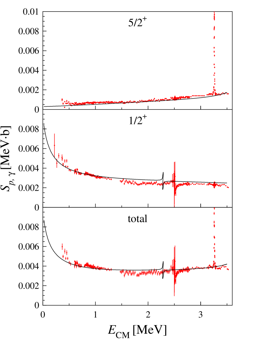
FIG. 7.: The astrophysical $S$-factor for the reactions ${}^{16}\mbox{O}(p,\gamma)^{17}\mbox{F}(J^{\pi}=5/2_{1}^{+})$ and ${}^{16}\mbox{O}(p,\gamma)^{17}\mbox{F}(J^{\pi}=1/2_{1}^{+})$ is plotted as a function of the center of mass energy $E_{CM}$. The experimental data are from [7]. The SMEC calculations (the solid line) have been done for the DDSM1 residual interaction (3). For more details see the description in the text.

FIG. 8.: The $E2$ and $M1$ components of the astrophysical $S$-factor for the reactions ${}^{16}\mbox{O}(p,\gamma)^{17}\mbox{F}(J^{\pi}=5/2_{1}^{+})$ (the dashed lines) and ${}^{16}\mbox{O}(p,\gamma)^{17}\mbox{F}(J^{\pi}=1/2_{1}^{+})$ (the solid lines) is plotted as a function of the center of mass energy $E_{CM}$. The SMEC calculations have been done for the DDSM1 residual interaction (3). For more details see the description in the text.

FIG. 9.: The phase-shifts for the $p+^{16}\mbox{O}$ elastic scattering as a function of the proton energy $E_{p}$ for the ${\frac{1}{2}}^{+}$, ${\frac{3}{2}}^{+}$, ${\frac{5}{2}}^{+}$, and ${\frac{1}{2}}^{-}$, ${\frac{3}{2}}^{-}$, ${\frac{7}{2}}^{-}$ partial waves. The experimental data are from [39]. SMEC results have been obtained for the DDSM1 residual interaction (3) and are plotted with the solid line. For ${\frac{5}{2}}^{+}$ partial wave, we show also the SMEC results without the resonant part (the dashed line). For more information see the description in the text.

FIG. 10.: The elastic cross-section at a laboratory angle $\theta_{LAB}=166^{\circ}$ for the $p+{{}^{16}\mbox{O}}$ scattering as a function of proton energy $E_{p}$. The SMEC calculations (the solid line) have been performed using the DDSM1 residual interaction. The results shown with the dashed line do not include the resonant contribution of $5/2_{1}^{+}$ state. Experimental cross-sections are from Ref. [40].

REFERENCES

- [1] T. Misu, W. Nazarewicz and S. Åberg, Nucl. Phys. A 614 (1997) 44.
- [2] K. Bennaceur, F. Nowacki, J. Okołowicz, and M. Płoszajczak, J. Phys. G 24 (1998) 1631.
- [3] K. Bennaceur, F. Nowacki, J. Okołowicz, and M. Płoszajczak, Nucl. Phys. A 651 (1999) 289.
- [4] H.W. Bartz, I. Rotter, and J. Höhn, Nucl. Phys. A 275 (1977) 111.
- [5] H.W. Bartz, I. Rotter, and J. Höhn, Nucl. Phys. A 307 (1977) 285.
-
[6]
H.R. Kissener, I. Rotter, and N.G. Goncharova, Fortschr. Phys. 35
(1987) 277;
I. Rotter, Rep. Prog. Phys. 54 (1991) 635. - [7] R. Morlock, R. Kunz, A. Mayer, M. Jaeger, A. Müller, J.W. Hammer, P. Mohr, H. Oberhummer, G. Staudt, and V. Kölle, Phys. Rev. Lett. 79 (1997) 3837.
- [8] C. Rolfs, Nucl. Phys. A 217 (1973) 29.
-
[9]
D. Baye, P. Descouvement and M. Hesse, Phys. Rev. C 58 (1998) 545;
P. Descouvement and D. Baye, Higher-order multipolarities in the and , to be published. - [10] C.R. Brune, Nucl. Phys. A 596 (1996) 122.
-
[11]
R. Wallace and S.E. Woosley, Astrophys. J., Suppl. Ser. 45 (1981) 389;
A.E. Champagne and M. Wiescher, Annu. Rev. Nucl. Part. Sci. 42 (1992) 39;
L. Van Wormer, J. Görres, C. Illiades, M. Wiescher and F.-K. Thielemann, Astrophys. J. 432 (1994) 326. -
[12]
K.E. Rehm et al., Phys. Rev. C 53 (1996) 1950;
M. Wiescher and K.U. Kettner, Astrophys. J. 263 (1982) 891. - [13] E.G. Adelberger et al., Rev. Mod. Phys. 70 (1998) 1265.
- [14] P. Descouvement and D. Baye, Nucl. Phys. A 487 (1998) 420; ibid. A 567 (1994) 341; A 573 (1994) 28.
- [15] A. Csótó, K. Langanke, S.E. Koonin, and J.D. Shoppa, Phys. Rev. C 52 (1995) 1130.
- [16] L.V. Grigorenko, B.V. Danilin, V.D. Efros, N.B. Shul’gina and M.V. Zhukov, Phys. Rev. C 57 (1998) R2099.
- [17] V.V. Balashov, A.N. Boyarkina, and I. Rotter, Nucl. Phys. 59 (1964) 414.
- [18] E. Caurier, code ANTOINE (unpublished).
- [19] B. Schwesinger and J. Wambach, Nucl. Phys. A 426 (1984) 253.
- [20] P.J. Brussard and P.W.M. Glaudemans, Shell Model Applications in Nuclear Spectroscopy, North Holland Publ. Comp. (Amsterdam, New York, Oxford).
- [21] C. Mahaux, and H. Weidenmüller, Shell-Model Approach to Nuclear Reactions (Amsterdam: North-Holland) (1969).
- [22] S. Cohen and D. Kurath, Nucl. Phys. A 73 (1965) 1.
-
[23]
B.M. Preedom and B.H. Wildenthal, Phys. Rev. C 6 (1972) 1633;
B.H. Wildenthal, Prog. Part. Nucl. Phys. 11 (1984) 5;
B.A. Brown, W.A. Richter, R.E. Julies and B.H. Wildenthal, Ann. Phys. (N.Y.) 182 (1988) 191;
B.A. Brown and B.H. Wildenthal, Annu. Rev. Nucl. Part. Sci. 38 (1988) 191. - [24] S. Kahana, H. C. Lee, and C. K. Scott, Phys. Rev 180 (1969) 956.
- [25] J. Duflo and A. P. Zuker Phys. Rev. C 59 (1999) R2347.
- [26] D. H. Gloeckner and R. D. Lawson, Phys. Lett. B 53 (1974) 313.
- [27] G.E. Brown and A.M. Green, Nucl. Phys. 75 (1966) 401.
- [28] A.P. Zuker, B. Buck and J.B. McGrory, Phys. Rev. Lett. 21 (1968) 39.
- [29] P. J. Ellis and L. Zamick, Annals of Physics (NY) 55 (1969) 61.
- [30] E. K. Warburton, J. A. Becker and B. A. Brown, Phys. Rev. C 41 (1990) 1147.
- [31] E.K. Warburton, B.A. Brown and D.J. Millener, Phys. Lett. B 293 (1992) 7.
- [32] E.K. Warburton and B.A. Brown, Phys. Rev. 46 (1992) 923.
- [33] W.C. Haxton and C. Johnson, Phys. Rev. Lett. 65 (1990) 1325.
- [34] D.J. Millener and D. Kurath, Nucl. Phys. A 255 (1975) 315.
- [35] M. Yasue et al., Phys. Rev. C 46 (1992) 1242.
- [36] H.J. Fortune, L.R. Medsker, J.P. Garrett, H.G. Bingham, Phys. Rev. C 12 (1975) 1723.
- [37] J. Vernotte, G. Berrier - Rosnin, J. Kalifa, R. Tamissier, and B.H. Wildenthal , Nucl. Phys. A 571 (1994) 1.
-
[38]
R.G. Thomas, Phys. Rev. 88 (1952) 1109;
J.B. Ehrman, Phys. Rev. 81 (1951) 412. - [39] R.A. Blue and W. Haeberli, Phys. Rev. 137 (1965) B284.
- [40] S.R. Salisbury, G. Haradie, L. Oppliger, and R. Dangle, Phys. Rev. 126 (1962) 2143.
- [41] E. Caurier, G. Martínez-Pinedo, F. Nowacki, A. Poves, J. Retamosa, and A. P. Zuker, Phys. Rev. C 59 (1999) 2033.