Boson spectra and correlations for thermal locally equilibrium systems

Abstract

The single- and multi- particle inclusive spectra for strongly inhomogeneous thermal boson systems are studied using the method of statistical operator. The thermal Wick’s theorem is generalized and the analytical solution of the problem for an boost-invariant expanding boson gas is found. The results demonstrate the effects of inhomogeneity for such a system: the spectra and correlations for particles with wave-lengths larger than the system’s homogeneity lengths change essentially as compared with the results based on the local Bose-Einstein thermal distributions. The effects noticeable grow for overpopulated media, where the chemical potential associated with violation of chemical equilibrium is large enough.

1 Introduction

The theoretical study of thermalized hadron and quark-gluon systems is important for understanding of the early Universe and new phenomena in the current and future experiments at SPS, RHIC and LHC. The systems formed in ultra-relativistic nucleus-nucleus collisions produce $10^{3}\div 10^{5}$ secondaries [1]. The number of quarks and gluons exceeds this estimate by one order of the value if the conditions for a phase transition to the QCD-plasma are realized. It is reasonable to expect that this quasi-macroscopic system could be thermalized during small proper time $\tau_{0\mbox{ }}$ after initial collision [2]. The systems formed in A+A collisions may be rather inhomogeneous ones even at the final decoupled stage $\tau=\tau_{f}$ of their evolution because of a strong expansion and very high initial density.

The current pion interferometry analysis at SPS CERN shows the effective sizes of such systems are $R\simeq 3\div 7$ $fm$ [3]. For a homogeneous static source the value $R^{2}$ is its geometrical mean-square size [4], for hydrodynamically expanding systems the longitudinal interferometry size is approximately proportional to the hydrodynamic length, $R_{L}\propto\lambda_{hydr}\equiv\left|v_{hydr,L}^{{}^{\prime}}\right|^{-1}\simeq\tau_{f},$ in a central rapidity region [5]. In general case the ”pion interferometry microscope” measures the lengths of homogeneity of hadron systems at the final stage. Naturally, for earlier stages, $\tau\leq\tau_{f}$, the effective geometrical or hydrodynamic lengths are smaller than the mentioned ones. At the initional stage of thermalization the typical hydrodynamic length (longitudinal length of homogeneity averaged over momenta ) is $\lambda_{hydr}\propto\tau_{0\mbox{ }}\simeq 1$ $fm$.

The statistical description of a quantum-field system with small homogeneity regions should be done carefully. As well known the statistical hydrodynamics can be based on the relativistic kinetic theory [6] as well as on the method of a nonequilibrium statistical operator [7]. In the both methods one uses the locally equilibrium distribution as the zero approximation. Then the complete Wigner function is usually represented by $f(x)=f_{0}(x,p)+\widetilde{f}(x,p)$ and nonequilibrium statistical operator is $\rho(\sigma)={\bf\rho(}\sigma)+\widetilde{\rho}(\sigma).$ Here $f_{0}(x,p)$ is a locally equilibrium distribution, the quasi-equilibrium statistical operator ${\bf\rho(}\sigma)$ is defined on some hypersurface $\sigma$ and corresponds to maximum entropy principle under a given set of additional conditions on local averages such as the energy density, the charge density, etc. The function $\widetilde{f}(x,p)$ and the operator $\widetilde{\rho}(\sigma)$ describe the nonequilibrium flows associated with a heat, viscosity, etc. They give the contributions that are roughly proportional to the ratio of the correlation length (mean free path) to the hydrodynamic length. As to the main approximation, the distribution function $f_{0}(x,p)$ is chosen usually in the form of globally equilibrium distribution with the substitutions: $T\rightarrow T(x)\equiv 1/\beta(x),v\rightarrow v_{hydr}(x)$, etc., where the parameters depend now on point $x$. This prescription is a physically self-consistent, if the hydrodynamic length is much more than the Compton (or de Broglie for massless fields) wavelengths $\lambda_{p}$ of the quanta, $\lambda_{p}\ll\lambda_{hydr}$ [6]. The condition cannot be satisfied for the effective mass $m\leq 0.1$ $GeV$ at the early stage, $\tau\simeq\lambda_{hydr}\approx 1fm$ , of the matter evolution in nucleus-nucleus collisions. One of the aims of this paper is to find the locally equilibrium function $f_{0}(x,p)$ in the general case of an arbitrary ratio $\lambda_{p}$ to $\lambda_{hydr}$. We shall use, for the purpose, the method of the quasi-equilibrium statistical operator [7], [8], [9].

The another problem, we discuss here, is how to calculate the two (many)- particles inclusive spectra for very inhomogeneous locally equilibrium systems. Strongly speaking, it is impossible to define the one-particle Wigner function in this case: the necessary condition that the thermal averages $<a^{\dagger}(p+\frac{q}{2})a(p-\frac{q}{2})>$ have to be diagonal enough, i.e. q${}_{eff}^{2}=\lambda_{hydr}^{-2}\ll m^{2}$[6], does not satisfied. In such a situation the direct use of the method of statistical operator is appropriate for the spectra calculation.

The special interest for discussion is the appearance of the additional terms in the double particle inclusive spectra connected with the non-zero averages of the products of the creation and annihilation operators, $\left\langle a^{+}a^{+}\right\rangle$ and $\left\langle aa\right\rangle$. Such terms have been obtained first for pions in the Gaussian current model [14]. The additional terms in the correlation function do not appear in the nonrelativistic quantum-mechanical approach [15]. We shall consider all these problems using the generalized Wick’s theorem for thermal locally equilibrium systems and give the explicit analytical structure of the pair-correlation function for different sorts of bosons.

In the section 2 we deal with the description of inclusive spectra in the standard Wigner’s representation and discuss some basic points of this approach.

In the section 3 we develop the statistical operator formalism for calculation of bosonic operator averages, $\left\langle a^{+}(p_{1})a(p_{2})\right\rangle$, $\left\langle a(p_{1})a(p_{2})\right\rangle$ , etc., in the locally equilibrium systems and discuss the physical conditions for the hydrodynamic solutions we are interested in.

In the section 4 the thermal Wick’s theorem is generalized for locally equilibrium systems. This is the basis for the calculation of the double- and multi- particle inclusive spectra.

The section 5 is devoted to the analytical calculation of the single particle spectra for a physically important case of the boost-invariant expansion of a hadron and/or quark-gluon matter. We derive there the correction term to the Bose-Einstein heat spectrum and demonstrate the tie of the term with the spectrum of the so-called Milne’s particles.

In the section 6 we obtain the structure of the pion-, kaon-, and photon- pair correlation functions. We calculate also the maximum value of the interferometry peak for these particles and the analytical approximation for the two-particle correlation function in typical experimental situations when $m{}{}{}\tau_{f}$ $\gg 1$.

2 The Statement of the Problem

The description of the inclusive spectra and correlations for a multiparticle production is based on a computation of the following type of the averages

$$p^{0}\frac{dN}{d{\bf p}}=\left\langle a_{p}^{+}a_{p}\right\rangle,\mbox{ }p_{1}^{0}p_{2}^{0}\frac{dN}{d{\bf p{\tt{}_{1}}}d{\bf p}{\tt{}_{2}}}=\left\langle a_{p_{1}}^{+}a_{p_{2}}^{+}a_{p_{1}}a_{p_{2}}\right\rangle,\mbox{ etc,...}$$ (1)

where $a_{p}^{+}$ and $a_{p}$ are the creation and annihilation operators, corresponding to a quantum field $\varphi_{out}(x,t)$ when an interaction is switched off. The brackets $<$…$>$ mean the average over some density matrix describing the state of the system on a some hypersurface $\sigma$. In the $S$-matrix theory the state is the $\left|out\right\rangle$-state at $\sigma:t=\infty$. In the statistical thermodynamic models of a multiparticle production the density matrix is chosen to be the statistical operator ${\bf\rho}$ and surface $\sigma$ is usually a freeze out hypersurface. The averages (1) taken on this hypersurface are coincided approximately with ones taken on an arbitrary hypersurface that situated within of the light cone of the future as to the freeze-out hypersurface. It corresponds to the preservation of the momentum distributions of free streaming particles in Eqs.(1) if one neglects the final state interaction and Coulomb corrections. The hypersurface $\sigma$ can correspond also to an earlier stage of the evolution if one studies the dilepton or photon productions from a hadron and/or quark-gluon plasma. It the latter case the operators $a_{p}^{+}$ and $a_{p}$ have to correspond to weekly interacting quasi-particles with the standard relativistic form of the dispersion relations in the medium and the masses depend now on the temperature and density. In this paper we shall not consider such a situation in details.

The inclusive double particle spectrum in (1) is usually calculated under supposition that the four-operator averages can be decomposed into the products of the irreducible two-operator ones

$$\left\langle a_{p_{1}}^{+}a_{p_{2}}^{+}a_{p_{1}}a_{p_{2}}\right\rangle=\left\langle a_{p_{1}}^{+}a_{p_{1}}\right\rangle\left\langle a_{p_{2}}^{+}a_{p_{2}}\right\rangle+\left\langle a_{p_{1}}^{+}a_{p_{2}}\right\rangle\left\langle a_{p_{2}}^{+}a_{p_{1}}\right\rangle$$ (2)

In this case the problem of the inclusive multi-particle spectra is reduced to the calculation of the $\left\langle a_{p_{1}}^{+}a_{p_{2}}\right\rangle$ averages.

If one considers the free identical particles 1 and 2 the two-operator average can be expressed by means of the following distribution function

$$f(x,p)=(2\pi)^{-3}\int d^{4}u\delta(p\cdot u)e^{-iu\cdot x}\left\langle a^{+}(p-\frac{u}{2})\;a(p+\frac{u}{2})\right\rangle$$ (3)

where $p=(p_{1}+p_{2})/2$ and the average is done in a space-time region where the interaction is negligible. Indeed, if we consider some hypersurface $\Sigma$ that situated in this region and can be closed by a plane surface $t=const$, it is possible to use the equation

$$\int d\Sigma_{\mu}p^{\mu}e^{ik\cdot x}=(2\pi)^{3}p^{0}e^{ik^{0}t}\delta^{3}({\bf k)}\mbox{ \qquad if \quad}p\cdot k=0$$ (4)

that follows from the Gauss theorem. Then

$$\begin{array}[]{l}\left\langle a^{+}(p_{1})a(p_{2})\right\rangle=\int d^{4}up^{0}e^{i(q^{0}-u^{0})t}\delta(p\cdot u)\delta^{3}({\bf q-u)}\left\langle a^{+}(p-\frac{u}{2})\;a(p+\frac{u}{2})\right\rangle\\ \\ =\int d\sigma_{\mu}p^{\mu}e^{iq\cdot x}f(x,p)\end{array}$$ (5)

Here $\sigma$ is the part of the hypersurface $\sum$ where $f(x,p)\neq 0$, $q=p_{2}-p_{1}.$

The expression (5) is general and describes the operator’s averages for the radiating matter when the hypersurface $\sigma$ is an arbitrary hypersurface situated within of the light cone of the future as to the decoupling 4-volume. In the general case the function $f(x,p)$ is rather complicated, even not positively defined. The distribution function $f(x,p)$ is coincided with the single- particle Wigner function $f_{W}(x,p)$ for free fields if $<a^{\dagger}(p+\frac{q}{2})a(p-\frac{q}{2})>$ is diagonal enough: $q_{eff}^{2}\ll m^{2}.$ Then there is the direct tie between the distribution function (3) and complete Wigner function $N(x,p)=\frac{1}{2}4\pi(2\pi)^{-5}\int d^{4}v\exp(-ipv)<:\varphi(x+\frac{1}{2}v)\varphi(x-\frac{1}{2}v):>$ [6].

The real calculations of the final spectra and correlations simplify greatly if a system is thermal and decoupling volume is narrow enough in time-like direction and so it can be considered as the freeze-out hypersurface. In this case one can use the thermal matrix density ${\bf\rho}$ at this freeze-out hypersurface $\sigma$ and calculate the phase-space distribution function $f(x,p)$ directly. When the surface $\sigma$ changes from event to event it is necessary to do the additional average over $\sigma$ in the all final expressions for spectra. But this procedure cannot be used even formally for description of two ( many)-particle spectra when the radiation volume is an essentially 4-dimensional one. For this aim instead of single particle Wigner function (let us suppose here that $f(x,p)=f_{W}(x,p)$) one have to use the quasi-classical density of particle emission $g(x,p)=p^{0}d^{7}N/d^{4}xd^{3}p$. The latter can be expressed by means of the derivation of complete Wigner function, $p^{\mu}\partial_{\mu}N(x,p)$, that take into account the interaction in the system leading to continuous radiation during some finite time. The decay of the resonances is one of an example of such a 4-volume emission. We will not consider this case in the paper.

As we show hereinafter, it is convenient to choose the one-component scalar field as the basic model of our consideration. The Lagrange function has the form  L=L${}_{KG}+$L_INT corresponding to the free Klein-Gordon field and an interaction term. If the latter is characterized by the coupling constant $\alpha$ (with the dimension equal to product of energy and volume), we can neglect the interaction energy and momentum if the following conditions for temperature $T$ and particle density $n(x)$ are satisfied [6]

$$\frac{n\alpha}{T}<<1$$ (6)

Neglecting the interaction terms, the single-particle Wigner function near the mass-shell is associated with the local current [6]. To be simple we will consider here the real field and use the particle flow as the current

$$j_{\mu}(x)=\varphi^{(+)}(x)\stackrel{{\scriptstyle\leftrightarrow}}{{\frac{\partial}{\partial x^{\mu}}}}\varphi^{(-)}(x)$$ (7)

where the decomposition of the field into ”positive” and ”negative” parts looks like

$$\varphi(x)=\varphi^{(+)}(x)+\varphi^{(-)}(x)\equiv[2(2\pi)^{3}]^{-\frac{1}{2}}\int\frac{d^{3}p}{p^{0}}\left[a_{p}^{+}e^{ip\cdot x}+a_{p}e^{-ip\cdot x}\right]$$ (8)

The expressions for the single particle spectrum and the double particle correlation function follow immediately from Eqs. (1),(2),(5):

$$p^{0}\frac{dN}{d{\bf p}}=\int d\sigma_{\mu}p^{\mu}f(x,p)$$ (9)

$$C(p_{1},p_{2})=1+\left(p_{1}^{0}p_{2}^{0}\frac{dN}{d{\bf p_{1}}}\frac{dN}{d{\bf p_{2}}}\right)^{-1}\left|\int d\sigma_{\mu}p^{\mu}e^{iq\cdot x}f(x,p)\right|^{2}$$ (10)

If one considers the infinite homogeneous thermodynamic system (with the chemical potential $\mu$, the energy-momentum operator $\widehat{P}$ and the operator of particle number $\widehat{N}$) that moves as a single whole with 4-velocity $u^{\mu}$, the result of the averaging over the equilibrium statistical operator

$${\bf\rho}_{eq}=\frac{1}{Z}\exp\left[\left(-\widehat{P}^{\nu}u_{\nu}+\mu\widehat{N}\right)/T\right]$$ (11)

is the following [6]

$$\left\langle a^{+}(p_{1})a(p_{2})\right\rangle=(2\pi)^{3}p^{0}f_{B.E.}(p)\delta^{3}({\bf p}_{1}-{\bf p}_{2})\mbox{, }\left\langle a(p_{1})a(p_{2})\right\rangle=0$$ (12)

where $f_{B.E.}(p)$ is the Bose-Einstein distribution for the globally-equilibrium systems. Let us put for simplicity $\mu=0$. Then

$$f(p,x)=\frac{(2\pi)^{-3}}{\exp(\beta p\cdot u)-1}\equiv f_{B.E.}(p;\beta,u);\,\beta=\frac{1}{T}=const,u^{\nu}=const.$$ (13)

Here the Wigner function does not depend on $x$. The thermal Wick’s theorem can be proved for a such type of systems, that leads to the result (2). The main approximation for the Wigner function of an expanding hadron and quark-gluon gas is usually based on the distributions like (13) with the substitutions $\beta=const\rightarrow\beta(x)$, $u=const\rightarrow u(x).$ Such substitutions are physically reasonable if the wavelength of the corresponding quanta, $\lambda_{p}=1/m_{eff}$, is much less than the hydrodynamic length

$$\lambda_{p}<<\lambda_{hydr}\propto\min\{\left|\partial^{\mu}u_{\mu}^{*}\right|^{-1},\left|gradT\right|^{-1}\}$$ (14)

Asterisk marks the values in the (local) rest system. As it was mentioned in Sec.1, the typical hydrodynamic length is approximately equal to the proper time of the hydrodynamic expansion, $\tau_{f}$ , and the inequality (14) is satisfied if $m\tau\gg$ $1$. For pions and kaons $m\tau_{f}\geq$1, for chiral quarks and gluons $m\tau\ll 1$. For thermalized photons there is always the momentum region where inequality (14) is strongly violated.

At the end of this section we would like to emphasize that the results (12), (13) for averages $\left\langle a_{p_{1}}^{+}a_{p_{2}}\right\rangle$ as well as the zero values for the averages $\left\langle a_{p_{1}}^{+}a_{p_{2}}^{+}\right\rangle$ have been derived for infinite homogeneous equilibrium systems only and cannot be automatically applied to locally equilibrium inhomogeneous system by using the simple substitution $\beta=const\rightarrow\beta(x)$, $u=const\rightarrow u(x)$ in the Bose-Einstein distribution (13). This concerns also of the two-particle spectra (10) and expansion (2) which is based on the Wick’s theorem for globally equilibrium systems.

It is interesting to mention that despite of the different structure of the correlation function (10) in different approaches (e.g.,[10, 11, 12, 13, 14]) they will give approximately same results being applied to systems that are quasi-homogeneous ones, $m\tau_{f}\gg 1,$ and are described by the same Wigner functions. But for strongly inhomogeneous systems it is impossible to introduce by a standard way the single particle Wigner function as well as to preserve the structure of the correlation function (10) based on Eq.(2). Therefore, all these approaches are off the region of their applicability. One have to calculate the averages such as $\left\langle a_{p_{1}}^{+}a_{p_{2}}\right\rangle$, $\left\langle a_{p_{1}}^{+}a_{p_{2}}^{+}\right\rangle$ directly. The formal distribution functions defined by (3) will be differ from local Bose-Einstein distribution even for ideal Bose gas. The structure (10) of the correlation function will be destroyed altogether with the Bose-Einstein distribution (13). In the following sections we propose the method for study of spectra and correlations in inhomogeneous thermal systems.

3 The Method of Locally Equilibrium Statistical Operator

The hydrodynamic description of quantum-field system, as known, can be based on the method of non-equilibrium statistical operator [7], [8], [9], [16]. The initial step in this method is to construct the so-called quasi-equilibrium statistical operator that describes hydrodynamics of the system neglecting the viscosity effects, heat conductivity, etc. In other words, the operator describes the locally equilibrium systems and since it will be used for this aim only we will call it as the locally equilibrium operator ${\bf\rho}$. To build the operator one usually applies the maximum entropy principle [7], [16]. The method carries into effect in a full analogy with the Gibbs method for homogenous equilibrium systems. In the latter case the set of the averages $<\widehat{E}>,$ $<\widehat{P}>,$ $<\widehat{Q}>,$ etc., is considered as the fixed additional conditions when the entropy $S$ is maximized. For the locally equilibrium systems considered on some hypersurface $\sigma$ with a time-like normal vector $n^{\nu}$ the collection of the additional conditions is based on densities of energy $\varepsilon(x)$, momentum ${\bf p}(x)$, charge $q(x)$, etc. In the relativistic covariant form they look like

$$\left\langle n_{\nu}(x)\widehat{T}^{\mu\nu}(x)\right\rangle,\quad\left\langle n_{\nu}(x)\widehat{J}^{\nu}(x)\right\rangle$$ (15)

where $\widehat{T}^{\mu\nu}(x)$ is the operator of the energy-momentum tensor, $\widehat{J}^{\nu}(x)$ is current density operator. According to the definition

$${\bf\rho=}e^{-S(\sigma)}$$ (16)

The entropy is maximized under the additional conditions like (15) by the Lagrange multipliers method

$$S=\max\;Sp\left[-{\bf\rho}\ln{\bf\rho-\rho}\int d\sigma\;n_{\gamma}(x)(\beta_{\nu}\widehat{T}^{\nu\gamma}(x)\;\;-\mu\beta\widehat{J}^{\gamma}(x))-\lambda{\bf\rho}\right]$$ (17)

where Lagrange multiplier $\beta_{\nu}(x)=u^{\nu}(x)/T(x)$ [16]. The formal solution of Eq.(17) gives us the result for entropy [9], [16]

$$S=S(\sigma)=\Phi(\sigma)+\int d\sigma\;n_{\gamma}(x)(\beta_{\nu}\widehat{T}^{\nu\gamma}(x)-\mu\beta\widehat{J}^{\gamma}(x))$$ (18)

where $\Phi(\sigma)=\ln\;Sp\exp\{\int d\sigma\;n_{\gamma}(x)(\beta_{\nu}\widehat{T}^{\nu\gamma}(x)-\mu\beta\widehat{J}^{\gamma}(x))\}$ is Masier-Planck functional. Let us put $\mu=0$ for simplicity. Sticking to the analogy with the method of statistical operator for globally equilibrium systems where all the operators under the sign $Sp$ are mutually commuted, we demand that

$$\;\left[\;n_{\nu}(x)\beta_{\mu}(x)\widehat{T}^{\mu\nu}(x)\;,\;\;n_{\gamma}(y)\beta_{\delta}(y)\widehat{T}^{\delta\gamma}(y)\right]_{\sigma}=0$$ (19)

In this case the set of the additional conditions (15) has the standard interpretation and we hope to avoid some mathematical difficulties that may possibly appear in a more general case.

As we mentioned in Sec.2, we shall start from the free one-component scalar field (8) with the standard commutation relations for the operators

$$\left[a(p),a^{+}(p^{\prime})\right]=p^{0}\delta^{3}({\bf p-p}^{\prime}{\bf)}$$ (20)

The energy-momentum tensor has the form

$$\widehat{T}^{\mu\nu}(x)=\frac{\partial\varphi}{\partial x_{\mu}}\frac{\partial\varphi}{\partial x_{\nu}}-g^{\mu\nu}{\cal L_{{\rm KG}}}$$ (21)

The commutation equation (19) is solved using the Eqs.(8), (20), (21) and gives the following conditions for hydrodynamic values taken on a hypersurface $\sigma:$

$$\begin{array}[]{l}n^{\mu}(x)=u^{\mu}(x)\\ \\ x\cdot u(x)=y\cdot u(y)\qquad\forall x,y\in\sigma\end{array}$$ (22)

It immediately follows from the Eqs.(22) that the commutation relation (19) is satisfied when one of the following conditions is realized:

1. The hypersurface $\sigma$ is plane and $u^{\mu}(x)=const$ ($v(x)=0$ in the reference system where $\sigma$ is $t=const$ ) . Actually, this means that the system occupies the space-time region with some distribution in temperature (falling down from central highly excited part to the vacuum at the periphery) and has no internal motion.

2. The hypersurface $\sigma$ is defined by the condition $t^{2}-{\bf x}_{L}^{2}=\tau^{2}=const$, and the one-dimensional expansion along $L$-axis occurs with 4-velocity $u_{0}=t/\tau$, $u_{L}=x_{L}/\tau,$ ${\bf u}_{T}=0.$ If $\beta$ is a constant on $\sigma$, it is reduced to the well-known boost-invariant expansion [17], [18], that is the basic model for application of the hydrodynamic theory to multiple processes in high energy collisions.

3. The hypersurface $\sigma$ is defined by the condition $t^{2}-{\bf x}_{T}^{2}=\tau^{2}=const$ and there holds the two-dimensional expansion $u_{0}=t/\tau$, ${\bf u}_{T}=x_{T}/\tau,$ $u_{L}=0$.

4. The hypersurface $\sigma$ is defined by the condition $t^{2}-{\bf x}^{2}=\tau^{2}=const$, 3-dimensional hydrodynamical expansion has the form $u^{\mu}=x^{\mu}/\tau$.

The method proposed to be used to find the averages of the operator products is based on the Gaudin’s idea [19] for globally equilibrium systems and is the following. We represent the locally-equilibrium statistical operator ${\bf\rho}$ defined by (16), (18) in the form

$${\bf\rho=}\frac{1}{Z}\exp\left[{\bf-}\int d\sigma_{\nu}\beta_{\mu}\widehat{T}^{\mu\nu}(x)\right]\qquad$$ (23)

where the integral is taken over corresponding hypersurface $\sigma$ as it was discussed before. Let us introduce the operators that dependent on some parameter $\alpha$ in the following way

$$\begin{array}[]{l}a^{+}(p,\alpha)=e^{{\bf-}\alpha\int d\sigma_{\nu}\beta_{\mu}\widehat{T}^{\mu\nu}(x)}a^{+}(p)\;e^{\alpha\int d\sigma_{\nu}\beta_{\mu}\widehat{T}^{\mu\nu}(x)}\\ \\ a(p,\alpha)=e^{{\bf-}\alpha\int d\sigma_{\nu}\beta_{\mu}\widehat{T}^{\mu\nu}(x)}a(p)\;e^{\alpha\int d\sigma_{\nu}\beta_{\mu}\widehat{T}^{\mu\nu}(x)}\end{array}$$ (24)

and use the matrix notation

$${\bf A(}p,\alpha)\equiv\left(\begin{array}[]{c}a^{+}(p,\alpha)\\ a(p,\alpha)\end{array}\right),\qquad{\bf A(}p)\equiv\left(\begin{array}[]{c}a^{+}(p)\\ a(p)\end{array}\right)$$ (25)

It is easy to get the following equations

$${\bf A(}p,\alpha=0)={\bf A(}p)$$ (26)

$$\begin{array}[]{c}<{\bf A(}p)a(p^{\prime})>=<a(p^{\prime}){\bf A(}p,\alpha=1)>\\ \\ <{\bf A(}p)a^{+}(p^{\prime})>=<a^{+}(p^{\prime}){\bf A(}p,\alpha=1)>\end{array}$$ (27)

The latter equations follow from the trace invariance under the cyclic permutation of operators. To express the operators ${\bf A(}p,\alpha)$ through $a^{+}(p)$ and $a(p)$ we shall use the equations that stem directly from Eq.(24)

$$\frac{\partial{\bf A(}p,\alpha)}{\partial\alpha}=e^{{\bf-}\alpha\int d\sigma_{\nu}\beta_{\mu}\widehat{T}^{\mu\nu}(x)}\left[{\bf A(}p)\;,\;\int d\sigma_{\nu}\beta_{\mu}\widehat{T}^{\mu\nu}(x)\right]e^{{\bf-}\alpha\int d\sigma_{\nu}\beta_{\mu}\widehat{T}^{\mu\nu}(x)}$$ (28)

Using the commutator (20) and conditions (22) we find the concrete form of Eq.(28) for scalar field (8)

$$\frac{\partial{\bf A(}p,\alpha)}{\partial\alpha}=\int d^{3}k{\bf K}(p,k){\bf A}(k,\alpha)$$ (29)

where the matrix kernel of integro-differential equation (29) has the form (asterisk means the complex conjugation)

$${\bf K}(p,k)=\left(\begin{array}[]{cc}G(p,k)&\overline{G}(p,k)\\ -\overline{G}^{*}(p,k)&-G^{*}(p,k)\end{array}\right)$$ (30)

where

$$\begin{array}[]{l}G(p,k)=-\frac{1}{(2\pi)^{3}}\int d\sigma\;e^{i(k-p)\cdot x}\frac{\beta(x)}{k^{0}}\left[k\cdot u\;p\cdot u-(k\cdot p-m^{2})/2\right]\\ \\ \overline{G}(p,k)=\frac{1}{(2\pi)^{3}}\int d\sigma\;e^{-i(k+p)\cdot x}\frac{\beta(x)}{k^{0}}\left[k\cdot u\;p\cdot u-(k\cdot p+m^{2})/2\right]\end{array}$$ (31)

Here $\beta(x)$ is the inverse of the local temperature $T(x)$, $u(x)=n(x)$ is the hydrodynamic 4-velocity and we use here the integral measure in the form $d\sigma_{\mu}=d\sigma\,n_{\mu}(x).$

The solution of the system of integro-differential equations (29), which is considered according to Eq.(26) as the Cauchy problem at ${\bf A(}p,\alpha=0)={\bf A(}p)$, is (see Ref.[20]):

$${\bf A(}p,\alpha)={\bf A(}p)+\sum_{n=1}^{\infty}\frac{\alpha^{n}}{n!}\int d^{3}k{\bf K}_{n}(p,k){\bf A(}k)$$ (32)

where ${\bf K}_{n}(p,k)$ is the $n$-th iteration of matrix kernel ${\bf K}$:

$$\begin{array}[]{l}{\bf K}_{1}(p,k)={\bf K}(p,k)\\ \\ {\bf K}_{n}(p,k)=\int ds_{1}ds_{2}...ds_{n-1}{\bf K}(p,s_{1}){\bf K}(s_{1},s_{2})...{\bf K}(s_{n-1},k)\end{array}$$ (33)

Using Eq.(30) we have the properties for the iterations of the kernel

$${\rm K_{n}^{22}}=(-1)^{n}{\rm K}_{n}^{*11},\quad{\rm K_{n}^{21}}=(-1)^{n}{\rm K}_{n}^{*12}$$ (34)

The system of integral equations for the operator averages follows from the solution (32) of the integro-differential equation (29) and the relation for averages (27):

$$\begin{array}[]{l}\sum_{n=1}^{\infty}\frac{1}{n!}\int d^{3}k\left({\rm K}_{n}^{11}(p,k)\left\langle a(p^{\prime})a^{+}(k)\right\rangle+{\rm K}_{n}^{12}(p,k)\left\langle a(p^{\prime})a(k)\right\rangle\right)=-p^{0}\delta^{3}(p-p^{\prime})\\ \\ \sum_{n=1}^{\infty}\frac{1}{n!}\int d^{3}k\left({\rm K}_{n}^{21}(p,k)\left\langle a(p^{\prime})a^{+}(k)\right\rangle+{\rm K}_{n}^{22}(p,k)\left\langle a(p^{\prime})a(k)\right\rangle\right)=0\end{array}$$ (35)

and

$$\begin{array}[]{l}\sum_{n=1}^{\infty}\frac{1}{n!}\int d^{3}k\left({\rm K}_{n}^{11}(p,k)\left\langle a^{+}(p^{\prime})a^{+}(k)\right\rangle+{\rm K}_{n}^{12}(p,k)\left\langle a^{+}(p^{\prime})a(k)\right\rangle\right)=0\\ \\ \sum_{n=1}^{\infty}\frac{1}{n!}\int d^{3}k\left({\rm K}_{n}^{21}(p,k)\left\langle a^{+}(p^{\prime})a^{+}(k)\right\rangle+{\rm K}_{n}^{22}(p,k)\left\langle a^{+}(p^{\prime})a(k)\right\rangle\right)=p^{0}\delta^{3}(p-p^{\prime})\end{array}$$ (36)

The integral equations (35) and (36) contain the complete information about the one- and many-particle inclusive spectra for the locally equilibrium thermalized Klein-Gordon field. If the system is an infinite homogeneous ($\beta$=const ) one and is considered on a flat hypersurface $\sigma$: $t_{\ast}=const$ in the rest frame where $u_{\ast}^{\mu}$ $=const$, it immediately follows from (31), (33) that ${\rm K}^{11}=-\beta p_{\ast}^{0}\delta^{3}({\bf p^{\ast}-k^{\ast})}$, ($p_{0}^{\ast}=p\cdot u),$ and according to Eqs. (35) and (36) we have

$$\left\langle a^{+}(p)a^{+}(p^{{}^{\prime}})\right\rangle_{eq}=\left\langle a(p)a(p^{\prime})\right\rangle_{eq}=0,\,\left\langle a^{+}(p)a(p^{{}^{\prime}})\right\rangle_{eq}=\frac{p^{0}\delta^{3}({\bf p-p^{{}^{\prime}})}}{\exp(\beta p\cdot u)-1}$$ (37)

This corresponds to the standard result (12) for globally equilibrium systems and leads to the Bose-Einstein distribution for a homogeneous ideal gas. In all other cases the result will be different from (37); the averages $\left\langle a^{+}a^{+}\right\rangle$ and $\left\langle aa\right\rangle$ do not vanish because $c$-factors attached to the corresponding operator pairs in the tensor $T^{\mu\nu}$ do not become zero after the integration over $\sigma$. Hereinafter we shall consider the solution of Eqs.(35) and (36) for the concrete locally equilibrium systems.

4 The Thermal Wick’s Theorem for Locally Equilibrium Systems

The double and multi-particles inclusive spectra are defined by Eqs.(1) and are expressed through the four and many operator averages. If a system is in globally equilibrium state, there can be used the thermal Wick’s theorem to express the many-point operator averages as the products of two point ones. For 4-point average the corresponding expansion is given by the Eq.(2). Our task now is to generalize thermal Wick’s theorem for locally equilibrium systems.

Let us consider the 4-point operator averages. First we introduce the notation for the operator expression

$$\sum_{n=1}^{\infty}\frac{1}{n!}\int d^{3}k{\rm K}_{n}(p,k)=\widehat{K}(p,k)$$ (38)

in order to simplify computation. Then the integral equations (35) and (36) take the compact form

$$\begin{array}[]{c}\widehat{K}(p,k)\left\langle a(p^{\prime}){\bf A(}k)\right\rangle=\left(\begin{array}[]{c}-p^{0}\delta^{3}({\bf p-p^{\prime})}\\ 0\end{array}\right)\\ \\ \quad\widehat{K}(p,k)\left\langle a^{+}(p^{\prime}){\bf A(}k)\right\rangle=\left(\begin{array}[]{c}0\\ p^{0}\delta^{3}({\bf p-p^{\prime})}\end{array}\right)\end{array}$$ (39)

Using the trace invariance under the cyclic permutation and solution (32) one can get convinced that

$$\begin{array}[]{l}\left\langle{\bf A(}p_{1})a^{+}(p_{2})a(p_{1}^{\prime})a(p_{2}^{\prime})\right\rangle=\left\langle a^{+}(p_{2})a(p_{1}^{\prime})a(p_{2}^{\prime}){\bf A(}p_{1},\alpha=1)\right\rangle=\\ \\ \left\langle a^{+}(p_{2})a(p_{1}^{\prime})a(p_{2}^{\prime}){\bf A(}p_{1})\right\rangle+\widehat{K}(p_{1},k)\left\langle a^{+}(p_{2})a(p_{1}^{\prime})a(p_{2}^{\prime}){\bf A(}k)\right\rangle\end{array}$$ (40)

After the commutation of the vector ${\bf A}$ and the representation of the arising $\delta$-function by means of the Eq.(39) we have

$$\begin{array}[]{l}\left\langle{\bf A(}p_{1})a^{+}(p_{2})a(p_{1}^{\prime})a(p_{2}^{\prime})\right\rangle-\left\langle a^{+}(p_{2})a(p_{1}^{\prime})a(p_{2}^{\prime}){\bf A(}p_{1})\right\rangle=\\ \\ \widehat{K}(p_{1},k){\tt[}\left\langle a(p_{1}^{\prime}){\bf A(}k)\right\rangle\left\langle a^{+}(p_{2})a(p_{2}^{\prime})\right\rangle+\left\langle a^{+}(p_{2}){\bf A(}k)\right\rangle\left\langle a(p_{1}^{\prime})a(p_{2}^{\prime})\right\rangle+\\ \\ \left\langle a(p_{2}^{\prime}){\bf A(}k)\right\rangle\left\langle a^{+}(p_{2})a(p_{1}^{\prime})\right\rangle]=\widehat{K}(p_{1},k)\left\langle a^{+}(p_{2})a(p_{1}^{\prime})a(p_{2}^{\prime}){\bf A(}k)\right\rangle\end{array}$$ (41)

Just in a similar way one can derive the analogous equation using the substitution $a^{+}(p_{2})\rightarrow a(p_{2})$ and the Hermitian conjugated to it. It is also worthy to mention that the equality between the last two parts of Eq.(41) is preserved when the vector ${\bf A}$ commutes to the left side in all the brackets. The Eq.(41) is easy generalized for the case of any even number of the operators by the induction method. All that means that the following equation is valid for even number of operators

$$\widehat{K}(p_{1},k){\bf\Delta}\left({\bf A(k),}A(p_{2}),...,A(p_{j}),...\right)={\bf 0}$$ (42)

where

$${\bf\Delta}=\left\langle{\bf A(k)}A(p_{2})...A(p_{j})...\right\rangle-\sum_{{\cal P}}\left\{\left\langle{\bf A(k)}A(p_{j_{k}})\right\rangle\prod\limits_{j^{\prime}>\,j;j,\;j,\prime\neq j_{k}}\left\langle A(p_{j}A(p_{j^{/}})\right\rangle\right\}$$ (43)

and $A(p)$ is $a^{+}(p)$ or $a(p)$ and ${\cal P}$ is the permutation sign. If the integral operator $\widehat{K}$ is a nondegenerate one, the Eq. (43) has the unique solution ${\bf\Delta=0}$ that means the average of any even number of operators expands in the sum of the products of all operator pairs taken in the same order as they were in the initial expression:

$$\left\langle A(p_{1})A(p_{2})...A(p_{n})\right\rangle=\sum_{{\cal P}}\prod\limits_{j^{\prime}>\,j}\left\langle A(p_{j}A(p_{j^{\prime}})\right\rangle,\qquad(n=2k)$$ (44)

It is obvious that the averages of odd numbers of the operators are equal to zero because of the bilinearity of the energy-momentum tensor $T^{\mu\nu}(x)$ in operators $a^{+},a$. So, the theorem is proved. The main peculiarity as compared with the standard results is the presence of additional terms like $\left\langle a^{+}(p_{1})a^{+}(p_{2})\right\rangle$ and $\left\langle a(p_{1})a(p_{2})\right\rangle$ in the expansion. As it will be shown in the next section these non-zero terms arise because of a space-time finiteness of the homogeneity regions in locally equilibrium systems.

5 Boson Spectra in the Boost-Invariant Hydrodynamic Model

In this section we consider the non-trivial case of a locally equilibrium system satisfying the conditions (22). It corresponds to the well-known and the physically important hydrodynamical solution of the 1D boost-invariant expansion [18].

Let us introduce the standard variables to analyze this hydrodynamic solution. The space-time variables in terms of rapidity $y$ and proper time of the expansion $\tau$ look as follows

$$t=\tau\cosh y,x_{L}=\tau\sinh y,u^{0}=\cosh y,u_{L}=\sinh y,d\sigma^{\mu}=u^{\mu}\tau d^{2}x_{T}dy$$ (45)

The system is considered on the hypersurface $\tau=const$, where the inverse of temperature $\beta=const.$

The particle momentum can be also expressed in terms of the particle longitudinal rapidity:

$$\begin{array}[]{c}p=\left(m_{p}\cosh\theta_{p},{\bf p}_{T},m_{p}\sinh\theta_{p}\right)\quad,\quad m_{p}\equiv m_{T}(p)=\sqrt{m^{2}+{\bf p}_{T}^{2}}\\ \\ d^{3}p=m_{p}\cosh\theta_{p}d^{2}p_{T}d\theta_{p};\\ \\ \left[a(p),a^{+}(p^{\prime})\right]=\left[a({\bf p}_{T},\theta_{p}),a^{+}({\bf p}_{T}^{\prime},\theta_{p^{\prime}})\right]=\delta^{2}({\bf p}_{T}-{\bf p}_{T}^{\prime})\delta(\theta_{p}-\theta_{p^{\prime}})\end{array}$$ (46)

To simplify the problem let us assume the transverse radius of the hydrodynamic tube to be much larger than the hydrodynamic length $\tau$. So one can neglect the influence of a finite transverse size of the system on the form of spectra. The calculation of the basic functions (31), $G$ and $\overline{G}$, that is easy to do using the variables (45), (46) with an infinite transverse region, give us the following results

$$G(p,k)=-\frac{m_{k}\tau\beta}{2\pi\cosh\theta_{k}}\delta^{2}({\bf p}_{T}-{\bf k}_{T})\int\limits_{-\infty}^{\infty}dz\sqrt{z^{2}+1}\exp\left[i2m_{k}\tau z\sinh\left(\frac{\theta_{p}-\theta_{k}}{2}\right)\right]$$ (47)

$$\overline{G}(p,k)=\frac{m_{k}\tau\beta}{\pi\cosh\theta_{k}}\delta^{2}({\bf p}_{T}+{\bf k}_{T})\int\limits_{1}^{\infty}dz\sqrt{z^{2}-1}\exp\left[-i2m_{k}\tau z\cosh\left(\frac{\theta_{p}-\theta_{k}}{2}\right)\right]$$ (48)

The functions (47), (48) are the distributions (the generalized functions). For example, for globally equilibrium systems $G(p,k)\propto\delta^{3}({\bf p-k)}$. They can be considered as the Fourier transforms of the distributions $\sqrt{1+z^{2}\mbox{ }}$ and $\theta(z-1)\sqrt{z^{2}-1}$ acting in the space of rapidly decreasing functions $f(\theta)$. According to the general rules of the operations with the so-called tempered functions [21], we shall mean or directly substitute the regular functions

$$G_{\epsilon}=G\left(\sqrt{1+z^{2}}\rightarrow e^{-\epsilon\left|z\right|}\sqrt{1+z^{2}}\right)\;,\;\overline{G}_{\epsilon}=\overline{G}\left(\sqrt{z^{2}-1}\rightarrow e^{-\epsilon\left|z\right|}\sqrt{z^{2}-1}\right)$$ (49)

instead of (47), (48) and use limit $\epsilon\rightarrow 0$ in the final expressions.

Let us rewrite the integral equations (35) in the variables (45), (46). Note that the element ${\rm K}_{n}^{ij}$ of the $n$-th iteration of the matrix kernel consists of even number ${\rm K}^{12}$ or ${\rm K}^{21}$ in Eq. (33) if $i=j$ and odd number of them if $i\neq j$. So taking into account the structure of the operators $G$ and $\overline{G}$, the solution of the integral equations (35) can be presented in the form

$$\left\langle a(p)a^{+}(k)\right\rangle={\cal A}_{1}(\theta_{p}-\theta_{k})\delta^{2}({\bf p}_{T}-{\bf k}_{T}),\;\left\langle a(p)a(k)\right\rangle={\cal A}_{2}(\theta_{p}-\theta_{k})\delta^{2}({\bf p}_{T}+{\bf k}_{T})$$ (50)

Then we have after the integration of Eq.(35) over $d^{2}{\bf k}_{T}$

$$\sum_{n=1}^{\infty}\frac{1}{n!}\int d\theta_{k}{\bf K}_{n}(\theta_{p}-\theta_{k}){\cal A}(\theta_{k}-\theta_{p^{\prime}})=\left(\begin{array}[]{c}-\delta(\theta_{p}-\theta_{p^{\prime}})\\ 0\end{array}\right)$$ (51)

here the matrix ${\cal A}=({\cal A}_{1},{\cal A}_{2})$ is defined by Eq.(50) and ${\bf K}_{n}(\theta_{p}-\theta_{k})$ are the $n$-th iteration of the kernel

$${\bf K}(\theta_{p}-\theta_{k})=\left(\begin{array}[]{cc}G(\theta_{p}-\theta_{k})&\overline{G}(\theta_{p}-\theta_{k})\\ -\overline{G}^{*}(\theta_{p}-\theta_{k})&-G^{*}(\theta_{p}-\theta_{k})\end{array}\right)$$ (52)

The matrix elements in (52) are defined by Eqs. (47),(48):

$$\begin{array}[]{l}G(\theta_{p}-\theta_{k})\delta^{2}({\bf p}_{T}-{\bf k}_{T})=m_{T}\cosh\theta_{k}G(p,k)\\ \mbox{ }\\ \overline{G}(\theta_{p}-\theta_{k})\delta^{2}({\bf p}_{T}+{\bf k}_{T})=m_{T}\cosh\theta_{k}\overline{G}(p,k)\end{array}$$ (53)

Fourier transform of Eq.(51) gives

$$\left[\exp{\bf K}(t)-{\bf I}\right]{\cal A}(t)=\left(\begin{array}[]{c}-1\\ 0\end{array}\right)$$ (54)

where I is unit matrix, ${\bf K}(t)$ is Fourier-transformed matrix (53).

The solution of the Eq.(54) is easy to find after the diagonalization of the ${\bf K(}t)$-matrix. The proper values of the corresponding characteristic equations are

$$\omega_{1}=-\omega(t),\;\omega_{2}=\omega(t)\equiv\sqrt{G^{2}(t)-\overline{G}^{*}(t)\overline{G}(t)}$$ (55)

and the matrix U transforming the coordinates ${\cal A}_{1}{\cal\ }$and ${\cal A}_{2}$ of the vector ${\cal A}$ to the new ones ${\cal A}_{1}^{\prime{\cal\ }}$and ${\cal A}_{2}^{\prime}$ and with the diagonal matrix ${\bf K}$ has the form

$$U\propto\left(\begin{array}[]{cc}(G-\omega)^{2}&(G-\omega)\overline{G}\\ (G-\omega)\overline{G}^{*}&(G-\omega)^{2}\end{array}\right)$$ (56)

Now one can get the solution of the Eq.(54). It is the following

$$\left\langle a^{+}a\right\rangle_{t}={\cal A}_{1}-1=\frac{1}{\exp\omega-1}\frac{(G-\omega)^{2}+\overline{G}^{*}\overline{G}\exp\omega}{(G-\omega)^{2}-\overline{G}^{*}\overline{G}}$$ (57)

$$\left\langle aa\right\rangle_{t}={\cal A}_{2}=-\frac{\overline{G}^{*}(G-\omega)}{(G-\omega)^{2}-\overline{G}^{*}\overline{G}}\frac{1+\cosh\omega}{\sinh\omega}$$ (58)

Before we will analyze the analytical structure of the Fourier components (57) and (58) of the pair operator averages, it is necessary to consider the principal problem. According to the construction of the matrix density ${\bf\rho}$ (23) the physical vacuum defined as $a\left|0\right\rangle=0$ is not the proper vector of $\rho$ because of the presence of the terms proportional to $a^{+}a^{+}$ in the energy-momentum tensor. The last term does not vanish after the integration over $d\sigma$ except for the case $\sigma$: $t=const,$ $\beta=const$. This means that at zero temperature, in the limit $\beta\rightarrow\infty$ ($T\rightarrow 0$), the operator averages such as (57) and (58) do not describe the modes of the physical vacuum $\left|0\right\rangle$ but is associated with the modes of some ”lowest” state $\left|0^{\prime}\right\rangle$ of the operator $\int d\sigma_{\nu}\beta_{\mu}\widehat{T}^{\mu\nu}(x)$. So all the exciting modes at finite temperature appear over background state $\left|0^{\prime}\right\rangle$ and we have to renormalize the averages:

$$\left\langle a^{+}a\right\rangle_{t}^{ren}=\left\langle a^{+}a\right\rangle_{t}-\left\langle a^{+}a\right\rangle_{t}^{\beta\rightarrow\infty}=(\exp\omega-1)^{-1}(1+2\left\langle a^{+}a\right\rangle_{t}^{\beta\rightarrow\infty}),etc,..$$ (59)

After this important remark we have finally

$$\left\langle a^{+}a\right\rangle_{t}^{ren}=\frac{1}{\exp\omega-1}\frac{\left|G\right|}{\omega},\;\left\langle aa\right\rangle_{t}^{ren}=\frac{1}{\exp\omega-1}\frac{\overline{G}^{*}}{\omega},\;\left\langle a^{+}a^{+}\right\rangle_{t}^{ren}=\frac{1}{\exp\omega-1}\frac{\overline{G}}{\omega}$$ (60)

where $\omega$ is defined by Eq.(55) and

$$\begin{array}[]{l}G(t)=-\frac{m_{T}^{2}\beta\tau}{\pi}\int dx\sqrt{1+x^{2}}\int d\theta e^{i2m_{T}\tau\,x\sinh\theta+\,i2t\theta}\\ \\ =-\frac{\beta\cosh(\pi t)}{\pi\tau}\int\limits_{0}^{\infty}dz\sqrt{(2m_{T}\tau)^{2}+z^{2}}K_{i2t}(z)\end{array}$$ (61)

$$\begin{array}[]{l}\overline{G}(t)=\mbox{ }\lim_{\epsilon\rightarrow 0}\frac{m_{T}^{2}\beta\tau}{\pi}\int d\theta e^{it\theta}\int\limits_{1}^{\infty}dz\sqrt{z^{2}-1}e^{-i2m_{T}\tau\,z\cosh\frac{\theta}{2}-\epsilon\,z}\\ \\ =im_{T}\beta\int d\theta\frac{e^{i2t\theta}}{2\cosh\theta}H_{1}^{(2)}(2m_{T}\tau\cosh\theta)\end{array}$$ (62)

Here $K_{\nu}$ is the modified Bessel function and $H_{1}^{(2)}(z)$ is the Hankel function of second order. The functions $G(t)$ and $\overline{G}(t)$ exhibit the following asymptotic behavior:

• $m_{T}\tau\gg 1$

  $$\begin{array}[]{l}G(t)\cong-\beta m_{T}[\sqrt{1+t^{2}/(m_{T}\tau)^{2}}+\frac{1}{24(m_{T}\tau)^{2}}\left(1+t^{2}/(m_{T}\tau)^{2}\right)^{-\frac{5}{2}}\times\\ \\ (1+\frac{3t}{m_{T}\tau}+\frac{t^{2}}{(m_{T}\tau)^{2}})+O((m_{T}\tau)^{-4})]\end{array}$$ (63)

  $$\left|\overline{G}(t)\right|\cong\beta m_{T}\left[\frac{1}{2m_{T}\tau}\left(1+t^{2}/(m_{T}\tau)^{2}\right)^{-1}+O((m_{T}\tau)^{-2})\right]$$ (64)

$$\omega(t)\cong\beta m_{T}\left(1+t^{2}/(m_{T}\tau)^{2}-\frac{1-3t/2m_{T}\tau-t^{2}/2m_{T}\tau}{6(m_{T}\tau)^{2}\left(1+t^{2}/(m_{T}\tau)^{2}\right)^{2}}\right)^{\frac{1}{2}}$$ (65)

• $m_{T}\tau\ll 1,\;t\leq m_{T}\tau$

  $$G(t)\cong-\frac{t\beta\coth\pi t}{\tau}\left\{1+\frac{(m_{T}\tau)^{2}}{2}\left[\ln{}^{2}\frac{m_{T}\tau}{2}+\ln\frac{m_{T}\tau}{2}+1\right]\right\}+O\left((m_{T}\tau)^{4}\right)$$ (66)

  $$\begin{array}[]{l}\overline{G}(t)\cong-\frac{t\beta}{\tau\sinh\pi t}\left\{1+\frac{(m_{T}\tau)^{2}}{2}\left[\ln{}^{2}\frac{m_{T}\tau}{2}+\ln\frac{m_{T}\tau}{2}+1-\pi^{2}\right]\right\}+\\ \\ +i\frac{\beta(m_{T}\tau)^{2}}{2\tau}\ln\frac{m_{T}\tau}{2}+O\left((m_{T}\tau)^{4}\right)\end{array}$$ (67)

  $$\omega(t)\cong\beta m_{T}\sqrt{1+t^{2}/(m_{T}\tau)^{2}}$$ (68)

The asymptotics is found by the saddle-point method for $m_{T}\tau\gg 1$ and using the representation of Eqs.(61), (62) as the sum of the hypergeometrical functions (see [22]) for $m_{T}\tau\ll 1$.

It is important to note that function $\omega$ is described by the expression (68) for all values $m_{T}\tau$ with the accuracy more than, at least, one percent as the numerical calculations have shown. It means, that the main factor $\left(\exp\omega-1\right)^{-1}$ in Eqs.(59) is actually the Bose-Einstein function (13). We believe that there is deep analytical foundation of this fact but we cannot explain this mathematical gift now.

It is worth to mention that the introduction of a non-zero chemical potential associated with violation of the chemical equilibrium in boson gas (overpopulation) leads to changing of all results by the substitution: $G(t)\rightarrow G(t)-\mu.$

Let us calculate the single particle spectrum for the case $\mu=0$. The pair operator average is described by the inverse Fourier transform of Eq.(60). With Eq.(50) taken into account we have

$$\left\langle a^{+}(p)a(p^{\prime})\right\rangle=\delta^{2}({\bf p}_{T}-{\bf p}_{T}^{\prime})\frac{1}{2\pi}\int dte^{-i(\theta_{p}-\theta_{p^{\prime}})t}\;\left\langle a^{+}a\right\rangle_{t}$$ (69)

$$\left\langle a(p)a(p^{\prime})\right\rangle=\left\langle a^{+}(p)a^{+}(p^{\prime})\right\rangle^{*}=\delta^{2}({\bf p}_{T}+{\bf p}_{T}^{\prime})\frac{1}{2\pi}\int dte^{-i(\theta_{p}-\theta_{p^{\prime}})t}\;\left\langle aa\right\rangle_{t}$$ (70)

One can calculate the formal distribution function defined by (3) using the variable $\zeta=$Ar$\sin$h$\frac{v_{L}}{2m_{T}\cosh\theta}$ and the representation (46) for momenta.

$$\begin{array}[]{l}f(x,p)_{\sigma}=\frac{2}{(2\pi)^{4}}\int d\zeta e^{i2m_{T}\tau\sinh(\theta-y)\sinh\zeta}\int dt\,e^{-i2t\zeta}\left\langle a^{+}a\right\rangle_{t}\\ \\ \approx\frac{\left\langle a^{+}a\right\rangle(t=m_{T}\tau\sinh(\theta-y))}{(2\pi)^{3}}\end{array}$$ (71)

The hydrodynamics rapidity $y$ defines the position of point $x$ according to Eq.(45). The last approximation in Eq.(71) is valid when the Fourier transform $F\left[\left\langle a^{+}a\right\rangle_{t}\right](\zeta)$ is fast decreasing in $\zeta$, that is satisfied. So in the local rest system of the fluid element, $y=0$, the result has the form

• $m_{T}\tau\gg 1$

  $$\frac{d^{6}N}{d^{3}xd^{3}p}_{|{\bf u=0}}=f(x,p)_{\sigma|{\bf u=0}}\approx\frac{(2\pi)^{-3}}{\exp(\beta p_{0})-1}\left(1+\frac{m_{T}^{2}}{24\tau^{2}p_{0}^{4}}\right)$$ (72)

• $m_{T}\tau\ll 1$

  $$\frac{d^{6}N}{d^{3}xd^{3}p}_{|{\bf u=0}}=f(x,p)_{\sigma|{\bf u=0}}\approx\frac{(2\pi)^{-3}}{\exp(\beta p_{0})-1}\frac{1}{\pi\tau p_{0}}=f_{BE}(p)\left(2f_{M}(p)\right)$$ (73)

We introduce here the designation

$$f_{M}(p)=\left\langle a^{+}a\right\rangle_{t=m_{T}\tau\sinh\theta}^{\beta\rightarrow\infty}+\frac{1}{2}=\left(e^{2\pi\tau p_{0}}-1\right)_{|\tau p_{0}\ll 1}^{-1}$$ (74)

The function $f_{M}(p)$ describes the ”heat” spectra with the ”temperature” $T_{eff}=1/2\pi\tau$ and the real temperature $T=0$ for the so-called Milne’s particles [23], which appear when the 2-dimensional field system is quantized in the hyperbolic space-time that is known as Milne’s Universe [24]. It happens due to the mixing of the positive and negative frequency components of a field in the hyperbolic world in compare with the Minkovski one. In the boost-invariant hydrodynamic model this hyperbolic space-time is formed by the isotherms. The state of the ”lowest” energy for the operator $\int d\sigma_{\nu}u_{\mu}\widehat{T}^{\mu\nu}$ containing in the statistical operator ${\bf\rho}$ was found in the Ref.[25] in the limit corresponding to $\tau\rightarrow 0$ in our case. So the unrenormalized spectrum $\left\langle a^{+}a\right\rangle_{t}^{\beta\rightarrow\infty}$ gives the standard result (74) for the spectrum of the Milne’s particles in this limit. After the background subtraction procedure, which is necessary since we study the particles against the background of the Minkovski vacuum but not the Milne’s one, the trace of this phenomenon can be observed at the finite temperature only as it is demonstrated by the Eqs.(59), (73). The physical reason for this lies in the creation of additional quanta of a bosonic field due to the interference of the positive and negative frequency components of a field when the latter begins to embrace the ”hyperbolically” expanding medium. Naturally this effect may be noticeable only if the wave-length of the quanta is much large than the length of homogeneity , in other words, when non-localized quanta ”feels” a space-time inhomogeneity of a medium.

The numerical demonstration of this effect for the distribution function is represented in Fig.1.

fig1sin.ps

Figure 1: The ratio of the boson phase-space distribution functions in expanding matter to the Bose-Einstein thermal distribution.

Note, that at $\mu\neq 0$ there is noticeable deviation of the distribution from the Bose-Einstein result even at $m_{T}\tau\gg 1$ that began to be very large when $\mu\rightarrow\mu_{cr}=m(1-1/2m\tau):$

$$\frac{f(p,x)}{f_{BE}(p,x)}\rightarrow\left(1-\frac{m_{T}^{2}}{(2\tau p_{0}(p_{0}-\mu))^{2}}\right)^{-1}$$ (75)

The single particle spectra according to (1),(69) for large enough radius $R$ of the hydrodynamic tube has the form

$$\frac{d^{2}N}{m_{T}dm_{T}d\theta}=\frac{\pi R^{2}}{(2\pi)^{3}}\int dt\left\langle a^{+}a\right\rangle_{t}$$ (76)

The effects of inhomogeneity will be important at the early stage, $\tau$$\approx 1$ fm for low-mass gluons or quasi-bosons if such objects there are at this stage. It could lead to the enhancement of photons and dileptons with low invariant mass. At the final freeze-out stage, even if $m_{T}\tau\gg 1$, the distortion of spectra due to the inhomoheneity will take place when the violation of the chemical equilibrium in boson gas is strong: the chemical potential $\mu$ is closed to $\mu_{cr}$.

Note, however, that we did not take into account a longitudional geometrical size of the system, $R_{L}.$ It means that our consideration is limited by the condition $p^{0}\geq 1/R_{L}.$ The condition $p^{0}\gg 1/R_{T}$ have been supposed before. Note, that as it was found in [26], a smallness of transverse geometrical size of the system, $R_{T}\leq 1/p^{0},$ leads to an reduction of number of soft quanta in locally equilibrium system in comparision with the Bose-Einstein spectra at the same values of thermodynamic parameters.

6 Two-Particle Correlations

The generalized Wick’s theorem (44) allows one to consider many-particle inclusive spectra and correlations for concrete fields. Let us begin from pion interferometry. The isotopic invariant Lagrangian of free pion field in the representation of real 3-component pion field operator $\pi$ and nonzero commutators have the form ($\;i,j=1,2,3.$):

$${\cal L}_{{\bf\pi}}=\frac{1}{2}\left({\bf\pi}_{;\mu}{\bf\pi}^{;\mu}\right)-\frac{m^{2}}{2}({\bf\pi\cdot\pi),\;}\left[\dot{\pi}_{j}(x^{0},{\bf x}),\pi_{j}(x^{0},{\bf x^{/}})\right]=\frac{1}{i}\delta_{j}^{i}\delta({\bf x-x^{/}})$$ (77)

So it is easy to see that dynamic equations split into three independent ones for each real component $\pi_{j}$; the statistical operator ${\bf\rho}$ is the product of three commuting exponents and all the previous results are preserved for each Hermitian field $\pi_{j}\Longleftrightarrow\varphi$ independently.

As it well known, the creation and annihilation operators of pions $\pi_{+},\pi_{-},\pi_{0}$ are described by the pion field in the complex representation and are connected with corresponding operators of the Hermitian ($\pi_{1},\pi_{2},\pi_{3\mbox{ }}$)-field in the following manner [27]

$$\begin{array}[]{ccc}a_{+}=\frac{1}{\sqrt{2}}\left(a_{1}+ia_{2}\right)&a_{+}^{+}=\frac{1}{\sqrt{2}}\left(a_{1}^{+}-\;ia_{2}^{+}\right)&a_{0}^{+}=a_{3}^{+}\\ a_{-}=\frac{1}{\sqrt{2}}\left(a_{1}-\;ia_{2}\right)&a_{-}^{+}=\frac{1}{\sqrt{2}}\left(a_{1}^{+}+\;ia_{2}^{+}\right)&a_{0}=a_{3}\end{array}$$ (78)

Using the Wick’s theorem (44) and Eq.(77) we express the inclusive spectra (1) through the results (69),(70),(60) for real scalar field taking into account that

$$\left\langle a_{i}^{+}a_{j}\right\rangle=\delta_{i}^{j}\left\langle a^{+}a\right\rangle,\,\left\langle a_{i}^{+}a_{j}^{+}\right\rangle=\delta_{i}^{j}\left\langle a^{+}a^{+}\right\rangle,\;\left\langle a_{i}\,a_{j}\right\rangle=\delta_{i}^{j}\left\langle a\,a\right\rangle$$ (79)

The results are

• for $\pi^{-}\pi^{-}$ (and similarly $\pi^{+}\pi^{+}$ ) pion pairs

  $$\begin{array}[]{r}\left\langle a_{+}^{+}(p_{1})a_{+}^{+}(p_{2})a_{+}(p_{1})a_{+}(p_{2})\right\rangle=\left\langle a^{+}(p_{1})a(p_{1})\right\rangle\left\langle a^{+}(p_{2})a(p_{2})\right\rangle\\ \\ +\left\langle a^{+}(p_{1})a(p_{2})\right\rangle\left\langle a^{+}(p_{2})a(p_{1})\right\rangle\end{array}$$ (80)

• for $\pi^{+}\pi^{-}$ pairs

  $$\begin{array}[]{r}\left\langle a_{+}^{+}(p_{1})a_{-}^{+}(p_{2})a_{+}(p_{1})a_{-}(p_{2})\right\rangle=\left\langle a^{+}(p_{1})a(p_{1})\right\rangle\left\langle a^{+}(p_{2})a(p_{2})\right\rangle\\ \\ +\left\langle a^{+}(p_{1})a^{+}(p_{2})\right\rangle\left\langle a(p_{2})a(p_{1})\right\rangle\end{array}$$ (81)

• for $\pi^{0}\pi^{0}$-pairs

  $$\begin{array}[]{c}\left\langle a_{0}^{+}(p_{1})a_{0}^{+}(p_{2})a_{0}(p_{1})a_{0}(p_{2})\right\rangle=\left\langle a^{+}(p_{1})a(p_{1})\right\rangle\left\langle a^{+}(p_{2})a(p_{2})\right\rangle\\ \\ +\left\langle a^{+}(p_{1})a(p_{2})\right\rangle\left\langle a^{+}(p_{2})a(p_{1})\right\rangle+\left\langle a^{+}(p_{1})a^{+}(p_{2})\right\rangle\left\langle a(p_{2})a(p_{1})\right\rangle\end{array}$$ (82)

Such a structure of the two pion spectra has been gotten in the Ref.[14] in the quantum optics model (Gaussian random sources) and in the Ref.[15] in two particle quantum mechanical approach. The significance of our result is that we calculate the averages $\left\langle a^{+}a\right\rangle,\,\left\langle a^{+}a^{+}\right\rangle$ and$\;\left\langle a\,a\right\rangle$ in the concrete realistic model of locally equilibrium hadron medium. The correlation function $C(p_{1},p_{2})$ for different pion pairs can be obtained by the division of the two particle spectra (80)-(82) by the single particle momentum distributions (79) of the corresponding pions. The theoretical maximum of the correlation functions $C(p_{1},p_{2})$ is achieved at ${\bf p}_{1}={\bf p}_{2}=0$ and can be easily estimated using the saddle point method:

$$\begin{array}[]{c}\max C(\pi^{\pm}\pi^{\pm})=2,\quad\max C(\pi^{\pm}\pi^{\mp})\approx 1+\left|\frac{\overline{G}(t=0)}{G(t=0)}\right|^{2},\\ \\ \;\max C(\pi^{0}\pi^{0})\approx 2+\left|\frac{\overline{G}(t=0)}{G(t=0)}\right|^{2}\end{array}$$ (83)

According to the asymptotic expansion (63)-(67)

$$\left|\frac{\overline{G}(t=0)}{G(t=0)}\right|^{2} \simeq \frac{m\beta}{(2m\tau)^{3}}\mbox{\ \ for\ \ }m\tau\gg 1$$ (84)

and

$$\mbox{\ \ \ }\left|\frac{\overline{G}(t=0)}{G(t=0)}\right|^{2} \simeq 1-(\pi m\tau)^{2}\mbox{\ \ for\ \ }m\tau\ll 1$$

The corresponding plot of $\max C(m\tau)$ is demonstrated in Fig. 2.

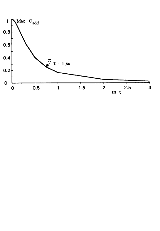
Figure 2: The aditional contribution to the correlation peak value for neutral and oppositely charged bosons at $\mu=0$.

For pions this value is noticeable only at $\tau\approx$1 fm and is 0.25 approximately, so $\max C_{\pi^{0}\pi^{0}}(\tau=1$fm$)\approx 2.25,$ $\max C_{\pi^{-}\pi^{+}}(\tau=1$fm$)\approx 1.25$. These values differ from the quantum-mechanical results [15] where $\max C_{\pi^{0}\pi^{0}}=2$, and $C_{\pi^{-}\pi^{+}}\equiv 1.$ This means that the effect has relativistic nature (decomposition of a field into the positive and negative frequency components and their interference in finite regions of homogeneity).

Note that if the chemical potential $\mu$ tends to critical value $\mu_{c}$ then even for large $m\tau\gg 1$ we have for maximal intercept (when the both quanta are very soft, ${\bf p}_{1}\simeq{\bf p}_{2}\simeq 0$) unusually large values: $\simeq 2$ for $\pi^{+}\pi^{-}$ and $\simeq 3$ for $\pi^{0}\pi^{0}$ . For equally charged pions $\pi^{+}\pi^{+}$ and $\pi^{-}\pi^{-}$ the intercept has the standard value =2 for any $m\tau$ and $\mu$.

In the typical experimental situation when $m\tau\gg 1$ and $\mu=0$ the Bose-Einstein correlation functions have the standard structure (10) for all sorts of identical pions and longitudinal projection of the correlation function can be approximated by the expression

$$C(p,q_{L};{\bf q}_{T}={\bf 0})\approx 1+\frac{\exp\left[\frac{2}{\lambda_{L}^{2}}\left(1-\sqrt{1+\tau^{2}\lambda_{L}^{4}q_{L}^{2}}\right)\right]}{\left(1+\tau^{2}\lambda_{L}^{4}q_{L}^{2}\right)^{3/2}}\stackrel{{\scriptstyle p_{T}\rightarrow\infty}}{{\longrightarrow}}1+\exp\left[-\tau^{2}\lambda_{L}^{2}q_{L}^{2}\right]$$ (85)

where $\lambda_{L}\approx\sqrt{\frac{T}{m_{T}}}.$ Here $T$ is the ”freeze out” temperature corresponding to proper time $\tau$ when the particles leave the expanding matter. This result is obtained by the saddle-point method from (80) and has the asymptotic form for longitudinal interferometry radius firstly obtained in Refs. [5], [13] for $\beta m_{T}\gg 1.$

The two- particle spectra for charge $K^{+},K^{-}$-kaons are described by Eqs. (80), (81) with substitution $\pi^{\pm}\rightarrow K^{\pm}$ because the complex representation for these fields can be replaced by the real one in the same manner as for charge pions. The same concerns of $K^{0},\overline{K}^{0}$-pairs. Because of relatively large kaon mass the role of the addition term in the correlation function $C(K^{+},K^{-})$ is negligible. For the correlation functions of identical kaons asymptotic form in Eq.(85) can be used in all momentum region.

The correlations in expanding photon gas are described by the formula (82) with multiplier $1/2$ at the second and third terms arising due to random polarization of photons. In this case the additional third term gives a good contribution for very soft photons producing $\max C=2$ instead of =1.5 without the third term.

7 Conclusions

In this paper we give the theoretical analyses of spectra and correlations in inhomogeneous weekly interacting boson gas. For the purpose the method of locally equilibrium statistical operator used to calculate the averages such as $\left\langle a^{+}(p_{1})...a(p_{j})...\right\rangle$ has been developed. The problem was reduced to the system of the integro-differential and integral equations solved analytically for physically significant model of hydrodynamic boost-invariant expansion. The main results are:

• the deviation of the particle phase-space density distribution from the Bose-Einstein one even in main approximation neglecting dissipative phenomena;

• the appearance of the additional terms in the correlation functions of like and unlike (oppositely charged) particles as compared with the results of the nonrelativistic quantum mechanical approach.

These effects are essential at small values $\tau p_{0}\leq 1$ or/and at large enough chemical potentials $\mu\rightarrow\mu_{c}$. Under this condition the ”effective” wave-length of the quanta, ($p_{0}-\mu$)^-1 is larger than the length of homogeneity $\tau$ in thermalized medium and quanta begin to ”feel” the all expanding matter. If $\mu=0,$ it results in the additional number of soft quanta due to interference of positive and negative frequency components of the relativistic quantum field in finite regions of homogeneity. In special case of Bjorken boost-invariant picture this effect is described by the spectrum $f_{M}(p_{0})$ of the so-called Milne’s particles that appear at zero temperature in the hyperbolic space-time due to a mixing of the positive and negative frequency field components relatively to the Minkovski space. In the hydrodynamic picture the role of the Milne’s Universe is played by the expanding thermalized matter ”forming” this hyperbolic world by the isoterms. Here there are no effects at zero temperature: the spectrum is $f(p_{0})=f_{BE}(p_{0})(2f_{M}(p_{0}))$. Note that Milne’s spectrum $f_{M}\propto\left|\left\langle aa\right\rangle\right|^{2}$. The last value is responsible for the additional terms in the correlation functions. Therefore, the both effects have the common nature. They are connected with the space-time inhomogeneity of systems.

The goal of the interferometry analysis in $A+A$ collisions is to study the space-time evolution of the matter or, roughly speaking, to find proper time $\tau$ of expansion. This is, actually, the average longitudinal length of homogeneity. Generally speaking, the ”interferometry microscope” measures the size and shape of homogeneity regions in radiating sources. As known, the relative smallness of the effective emitting region is the basic condition for interferometry method to be applied experimentally. Under this circumstance the taking into account of the new effects for spectra and correlations of effectively soft bosons, ($p_{0}-\mu$)${}^{-1}\gg\tau$ become to be important.

The experimental consequences of the effect in the ultra-relativistic nucleus-nucleus collisions could also concern of the particles with small mass such as chiral quarks, gluons, photons, etc. The theory predicts the essential enhancement for a number of particles with small effective energy at an early stage of the matter expansion. This can lead to the increase in the number of photons and dileptons with small transverse momenta or small invariant masses if they are produced in the collisions of particles with small effective mass.

Comments

The paper is minor modified version of the unpublished preprint Yu.M.Sinyukov, ITP-93-8E, Kiev, 1993. Here was done firstly the interpretation of the HBT radii as the lengths of homogeneity in radiating systems. The modification takes into account some of the later results published in proceedings of the conferences:

Yu.M.Sinyukov, Nucl. Phys. A566 (1994) 589c (QM 93);

Yu.M.Sinyukov. Spectra and correlations in small inhomogenious systems. In: Hot Hadronic Matter. Theory and Experiment, (J.Letessier, H.H.Gutbrod, J.Rafelski, eds.) p. 309, Plenum Publ., 1995. (NATO Workshop, Divonne-94);

Yu.M.Sinyukov, S.V.Akkelin, A.Yu.Tolstykh, Nucl.Phys. A610 (1996) 278c (QM 96);

Yu.M.Sinyukov, S.V.Akkelin, R.Lednicky, In Proc. of the 8th International Workshop on Maltiparticle Production in Matrahaza (T.Csorgo et al, eds), p.66, World Scientific, 1998.

and in the paper Yu.M.Sinyukov, B.Lorstad, Z.Phys.C61 (1994) 587. AcknowledgementI express my sincere thanks to V.A.Averchenkov for his assistance in the computer calculations and S.V.Akkelin for fruitful disscussions.

References

• [1] H.Satz: in LHC Workshop (Aachen) v.1, CERN 90-10,ECFA 90-133, Geneva, 1990.
• [2] H.von Gersdorff, L.McLerran, M.Kataja, P.V.Ruuskanen, Phys.Rev.D34 (1986) 794.
• [3] D.Ferenc, Nucl. Phys. A610 (1996) 523c.
• [4] G.I.Kopylov, M.I.Podgoretsky, Sov.J.Nucl.Phys.15 (1972) 392.
• [5] Yu.M.Sinyukov, Nucl.Phys.A498 (1989) 151c.
• [6] S.R.de Groot, W.A.van Leeuwen, Ch.G.van Weert: Relativistic Kinetic Theory, North-Holland, Amsterdam, 1980.
• [7] D.N.Zubarev: Nonequilibrium Statistical Thermodynamics,Nauka, Moscow, 1971
• [8] S.A.Smolyansky, A.D.Panferov: Introduction in Relativistic Statistical Hydrodynanics of Normal Fluid, Saratov University Press, Saratov, 1986.
• [9] A.D.Panferov, Yu.M.Sinyukov, S.A.Smolyanski, Preprint ITP-87-33E, Kiev, 1987.
• [10] S. Pratt, Phys.Rev.D33 (1986) 1314.
• [11] K.Kolehmanien, M.Gyulassy, Phys.Lett.B180 (1986) 203.
• [12] Y.Hama, S.S.Padula, Phys.Rev.D37 (1988) 3237.
• [13] A.N.Makhlin, Yu.M.Sinyukov, Sov.J.Nucl.Phys. 46 (1987) 345; V.A.Averchenkov, A.N.Makhlin, Yu.M.Sinyukov, Yadernaya Fizika 46 (1987) 1525.
• [14] I.V.Andreev, M.Plumer, R.M.Weiner, Phys.Rev.Lett.67 (1991) 3475.
• [15] Yu.M.Sinyukov, A.Yu.Tolstykh, Sov.J.Nucl.Phys.56 (1993) 184
• [16] Ch.G.von Weert, Ann.Phys.140 (1982) 133.
• [17] M.I.Gorenstein, Yu.M.Sinyukov, V.I.Zhdanov, Phys.Lett.B71 (1977) 199.
• [18] J.D.Bjorken, Phys.Rev.D27 (1983) 140.
• [19] M.Gaudin, Nucl.Phys.15 (1960) 89.
• [20] Ya.V.Bykov: On some Problems of the Theory of Integro-Differential Equations, Kirghiz State Univer-sity Press, Frunze, 1957.
• [21] H.Bremermann: Distributions, Complex Variables, and Fourier Transforms, Addison-Wesley, Reading, Massachusetts, 1965.
• [22] A.P.Prudnikov, Yu.A.Brychkov, O.I.Marichev: Integrals and Series. (Mathematical functions), Nauka, Moscow, 1983.
• [23] N.D.Birrel,P.C.W.Davies: Quantum Fields in Curved Space, Cambrige University Press, Cambrige, 1982.
• [24] E.A.Milne, Nature 130 (1932) 9.
• [25] C.M.Sommerfield, Ann.Phys.84 (1974) 285.
• [26] Yu.M. Sinyukov, S.V. Akkelin, R. Lednicky, in: Proceed. of the 8-th International Workshop on Multiparticle Production, eds. T. Csorgo et al, (World Scientific, 1998) p.66.
• [27] J.D.Bjorken, D.Drell, Relativistic Quantum Fields, Mc Graw-Hill Book Company, 1976.