Quadrupole deformations of neutron-drip-line nuclei studied within the Skyrme Hartree-Fock-Bogoliubov approach

Abstract

We introduce a local-scaling point transformation to allow for modifying the asymptotic properties of the deformed three-dimensional Cartesian harmonic oscillator wave functions. The resulting single-particle bases are very well suited for solving the Hartree-Fock-Bogoliubov equations for deformed drip-line nuclei. We then present results of self-consistent calculations performed for the Mg isotopes and for light nuclei located near the two-neutron drip line. The results suggest that for all even-even elements with $Z$=10–18 the most weakly-bound nucleus has an oblate ground-state shape.

]

I Introduction

Thanks to recent advancess in radioactive ion beam technology, we are now in the process of exploring the very limits of nuclear binding, namely those regions of the periodic chart in the neighborhood of the particle drip lines [1, 2, 3, 4]. Several new structure features have already been uncovered in these studies, including the neutron halo, and others have been predicted.

In contrast to stable nuclei within or near the valley of beta stability, a proper theoretical description of weakly-bound systems requires a very careful treatment of the asymptotic part of the nucleonic density. This is particularly true in the description of pairing correlations near the neutron drip line, for which the correct asymptotic properties of quasiparticle wave functions and of one-particle and pairing densities is essential. In the framework of the mean-field approach, the best way to achieve such a description is to use the Hartree-Fock-Bogoliubov (HFB) theory in coordinate-space representation [5, 6, 7].

Such an approach presents serious difficulties, however, when applied to deformed nuclei. On the one hand, for finite-range interactions the technical and numerical problems arising when a two-dimensional mesh of spatial points is used are so involved that reliable self-consistent calculations in coordinate space should not be expected soon. On the other hand, for zero-range interactions existing approaches [8, 9] are able to include only a fairly limited pairing phase space. The main complication in solving the HFB equations in coordinate space is that the HFB spectrum is unbounded from below, so that methods based on a variational search for eigenstates cannot be easily implemented. Because of this and other difficulties, one has to look for alternative solutions.

In principle, such an alternative solution is well known in the form of the configurational representation. In this approach, the system of partial differential HFB equations are solved by expanding the nucleon quasiparticle wave functions in an appropriate complete set of single-particle wave functions. In many applications, an expansion of the HFB wave function in a large harmonic oscillator (HO) basis of spherical or axial symmetry provides a satisfactory level of accuracy. For nuclei at the drip lines, however, expansion in an oscillator basis converges much too slowly to describe the physics of continuum states [7], which play a critical role in the description of weakly-bound systems. Oscillator expansions produce wave functions that decrease too steeply in the asymptotic region at large distances from the center of the nucleus. As a result, the calculated densities, especially in the pairing channel, are too small in the outer region and do not reflect correctly the pairing correlations of such nuclei.

In two recent works [10, 11], a new transformed harmonic oscillator (THO) basis, based on a unitary transformation of the spherical HO basis, was discussed. This new basis derives from the standard oscillator basis by a local-scaling point coordinate transformation [12, 13, 14], with the precise form dictated by the desired asymptotic behavior of the densities. The transformation preserves many useful properties of the HO wave functions. Using the new basis, characteristics of weakly-bound orbitals for a square-well potential were analyzed and the ground-state properties of some spherical nuclei were calculated in the framework of the energy density functional approach[11]. It was demonstrated in [10] that configurational calculations using the THO basis present a promising alternative to algorithms that are being developed for coordinate-space solution of the HFB equations.

In the present work, we develop the THO basis for use in HFB equations of axially-deformed weakly-bound nuclei. Our main goal here is to present and test these new theoretical methods. As specific applications, we repeat previous calculations performed for the chain of Mg isotopes [8], but for different effective interactions, and then report a preliminary study of light, neutron-rich nuclei near the drip line. Extensive calculations throughout the mass table, together with a more detailed analysis of the pairing interaction, will be presented in a future publication.

The structure of the paper is the following. The THO basis for deformed nuclei is introduced in Sec. II. In Sec. III we present an outline of the HFB theory and discuss several features of particular relevance to our investigation. Results of calculations are given in Sec. IV, and conclusions are presented in Sec. V.

II Transformed Harmonic Oscillator Basis

In this section, we introduce a generalized class of local-scaling point transformations, which in principle act differently in the three Cartesian directions. Next, we apply this transformation to the three-dimensional Cartesian HO wave functions and derive the corresponding properties of the local densities.

A Local-scaling point transformations

Suppose $\{\varphi_{\alpha}({\mathchoice{{\hbox{\boldmath$\displaystyle r$}}}{{\hbox{\boldmath$\textstyle r$}}}{{\hbox{\boldmath$\scriptstyle r$}}}{{\hbox{\boldmath$\scriptscriptstyle r$}}}})\}$ represents a complete set of orthonormal single-particle wave functions depending on the spatial coordinate $\textstyle r$. (To simplify the presentation, we suppress the spin and isospin labels here.) Then, one can introduce a local-scaling point transformation (LST) of the three dimensional vector space, which is a generalization of the analogous spherically-symmetric LST [12, 13, 14], namely

$$\begin{array}[]{ll}x\longrightarrow&x^{\prime}\equiv x^{\prime}(x,y,z)=\frac{x}{{r}}f_{x}({r}),\\ y\longrightarrow&y^{\prime}\equiv y^{\prime}(x,y,z)=\frac{y}{{r}}f_{y}({r}),\\ z\longrightarrow&z^{\prime}\equiv z^{\prime}(x,y,z)=\frac{z}{{r}}f_{z}({r}),\end{array}$$ (1)

where ${r}$=$\sqrt{x^{2}+y^{2}+z^{2}}$.

The LST functions $f_{k}({r})$, $k$=$x$, $y$, or $z$, should have mathematical properties ensuring that (1) is a valid invertible transformation of the three-dimensional space. In particular, $f_{k}({r})$ should be monotonic functions of ${r}$ such that

$$\begin{array}[]{lll}f_{k}(0)=0&\mbox{~{}~{}and~{}~{}}&f_{k}(\infty)=\infty\end{array},$$ (2)

and should lead to a non-vanishing Jacobian of the LST (1), i.e.,

$$D \equiv \frac{\partial(x^{\prime},y^{\prime},z^{\prime})}{\partial(x,y,z)}$$ (3)

$$= \frac{x^{2}f^{\prime}_{x}f_{y}f_{z}+y^{2}f_{x}f^{\prime}_{y}f_{z}+z^{2}f_{x}f_{y}f^{\prime}_{z}}{{r}^{4}}\neq 0,$$ (4)

where primes denote derivatives with respect to $r$.

When we apply the LST ( 1) to the set of wave functions $\varphi_{\alpha}({\mathchoice{{\hbox{\boldmath$\displaystyle r$}}}{{\hbox{\boldmath$\textstyle r$}}}{{\hbox{\boldmath$\scriptstyle r$}}}{{\hbox{\boldmath$\scriptscriptstyle r$}}}})$, we obtain another set of single-particle wave functions

$$\psi_{\alpha}(x,y,z)=D^{1/2}\varphi_{\alpha}\textstyle{\left(\frac{x}{{r}}f_{x}({r}),\frac{y}{{r}}f_{y}({r}),\frac{z}{{r}}f_{z}({r})\right)}.$$ (5)

Due to the factor $D^{1/2}$ entering Eq.(5), the LST of wave functions is unitary and the new wave functions $\psi_{\alpha}({\mathchoice{{\hbox{\boldmath$\displaystyle r$}}}{{\hbox{\boldmath$\textstyle r$}}}{{\hbox{\boldmath$\scriptstyle r$}}}{{\hbox{\boldmath$\scriptscriptstyle r$}}}})$ are automatically orthonormal, i.e., $\langle\psi_{\alpha}|\psi_{\beta}\rangle$=$\langle\varphi_{\alpha}|\varphi_{\beta}\rangle$=$\delta_{\alpha\beta}$.

Summarizing, the LST (1) generates from a given complete set of orthonormal single-particle wave functions another orthonormal and complete set of single-particle wave functions (5) depending on three almost-arbitrary scalar LST functions $f_{k}({r})$. The freedom in the choice of $f_{k}({r})$ provides great flexibility in the new set $\{\psi_{\alpha}({\mathchoice{{\hbox{\boldmath$\displaystyle r$}}}{{\hbox{\boldmath$\textstyle r$}}}{{\hbox{\boldmath$\scriptstyle r$}}}{{\hbox{\boldmath$\scriptscriptstyle r$}}}})\}$, and this opens up the possibility of improving on undesired properties of the initial set. This is the motivation for the present study in which we use the LST to modify the incorrect asymptotic properties of deformed HO wave functions.

B Transformed harmonic oscillator wave functions

The anisotropic three-dimensional HO potential with three different oscillator lengths

$$L_{k}\equiv\frac{1}{b_{k}}=\sqrt{\frac{\hbar}{m\omega_{k}}},$$ (6)

has the form

$$U({\mathchoice{{\hbox{\boldmath$\displaystyle r$}}}{{\hbox{\boldmath$\textstyle r$}}}{{\hbox{\boldmath$\scriptstyle r$}}}{{\hbox{\boldmath$\scriptscriptstyle r$}}}})=\frac{\hbar^{2}}{2m}\left(\frac{x^{2}}{L_{x}^{4}}+\frac{y^{2}}{L_{y}^{4}}+\frac{z^{2}}{L_{z}^{4}}\right).$$ (7)

Its eigenstates, the separable HO single-particle wave functions

$$\varphi_{\alpha}({\mathchoice{{\hbox{\boldmath$\displaystyle r$}}}{{\hbox{\boldmath$\textstyle r$}}}{{\hbox{\boldmath$\scriptstyle r$}}}{{\hbox{\boldmath$\scriptscriptstyle r$}}}})=\varphi_{n_{x}}(x)\varphi_{n_{y}}(y)\varphi_{n_{z}}(z),$$ (8)

have a Gaussian asymptotic behavior at large distances,

$$\varphi_{\alpha}({\mathchoice{{\hbox{\boldmath$\displaystyle r$}}}{{\hbox{\boldmath$\textstyle r$}}}{{\hbox{\boldmath$\scriptstyle r$}}}{{\hbox{\boldmath$\scriptscriptstyle r$}}}\rightarrow\infty})\sim\exp\left[-\frac{1}{2}\left(\frac{x^{2}}{L_{x}^{2}}+\frac{y^{2}}{L_{y}^{2}}+\frac{z^{2}}{L_{z}^{2}}\right)\right].$$ (9)

Applying the LST (1) to these wave functions leads to the so-called THO single-particle wave functions (5),

$$\psi_{\alpha}({\mathchoice{{\hbox{\boldmath$\displaystyle r$}}}{{\hbox{\boldmath$\textstyle r$}}}{{\hbox{\boldmath$\scriptstyle r$}}}{{\hbox{\boldmath$\scriptscriptstyle r$}}}})=D^{1/2}\textstyle{\ \varphi_{n_{x}}\left(\frac{x}{{r}}f_{x}({r)}\right)\varphi_{n_{y}}\left(\frac{y}{{r}}f_{y}({r)}\right)\varphi_{n_{z}}\left(\frac{z}{{r}}f_{z}({r)}\right)},$$ (10)

whose asymptotic behavior is

$$\psi_{\alpha}({\mathchoice{{\hbox{\boldmath$\displaystyle r$}}}{{\hbox{\boldmath$\textstyle r$}}}{{\hbox{\boldmath$\scriptstyle r$}}}{{\hbox{\boldmath$\scriptscriptstyle r$}}}\rightarrow\infty})\sim\exp\left[-\frac{1}{2}\left(\frac{x^{2}f^{2}_{x}}{L_{x}^{2}r^{2}}+\frac{y^{2}f^{2}_{y}}{L_{y}^{2}r^{2}}+\frac{z^{2}f^{2}_{z}}{L_{z}^{2}r^{2}}\right)\right].$$ (11)

This suggests that we choose the LST functions to satisfy the asymptotic conditions

$$f_{k}(r)=\left\{\begin{array}[]{cl}r&\mbox{~{}~{}~{}for small $r$},\\[4.30554pt] L_{k}\sqrt{2\kappa r}&\mbox{~{}~{}~{}for large $r$}.\end{array}\right.$$ (12)

With such a choice, the THO wave functions at small $r$ are identical to the HO wave functions (note that with (12) one obtains $D$=1 at small $r$), while at large $r$ they have the correct exponential and spherical asymptotic behavior,

$$\psi_{\alpha}({\mathchoice{{\hbox{\boldmath$\displaystyle r$}}}{{\hbox{\boldmath$\textstyle r$}}}{{\hbox{\boldmath$\scriptstyle r$}}}{{\hbox{\boldmath$\scriptscriptstyle r$}}}\rightarrow\infty})\sim e^{-\kappa r}.$$ (13)

C Parametrization of the LST functions

In principle, we could use the flexibility of having three different LST functions $f_{k}({r})$ and three different oscillator lengths $L_{k}$ of the original deformed HO basis to tailor the LST transformation to the shape of the deformed nucleus under investigation. However, for large HO bases (in the present study we include HO states up to 20 major shells), the dependence of the total energy on the basis deformation is very weak, so that minimization of the total energy with respect to the three oscillator lengths $L_{k}$ is ill-conditioned (see discussion and examples given in Ref. [15]). Therefore, in this study, we use a spherical HO basis depending on a single common oscillator length $L_{0}$,

$$L_{x}=L_{y}=L_{z}\equiv L_{0}=\frac{1}{b_{0}}=\sqrt{\frac{\hbar}{m\omega_{0}}}.$$ (14)

With such a choice, it is natural to set the three LST functions $f_{k}(r)$ equal to one another,

$$f_{x}({r})=f_{y}({r})=f_{z}({r})\equiv f({r}).$$ (15)

This allows us to use exactly the same LST function $f({r})$ as in the previous studies [10, 11]. Under conditions (15), the Jacobian (4) assumes the simpler form

$$D \equiv \frac{\partial(x^{\prime},y^{\prime},z^{\prime})}{\partial(x,y,z)}=\frac{f^{\prime}({r})f^{2}({r})}{{r}^{2}}.$$ (16)

The parametrization of the LST function $f({r})$ used in Refs. [10, 11] was of the form

$$f({r})=L_{0}F\left(\frac{r}{L_{0}}\right),$$ (17)

with the dimensionless universal function $F$ of the dimensionless variable ${\cal R}$ defined as

$$F({\cal R})\!=\!\left\{\!\!\begin{array}[]{lll}{\cal R}\left(1+a{\cal R}^{2}\right)^{1/3}&\mbox{for}&{\cal R}\leq c\;,\\ &&\\ \sqrt{\frac{d_{-2}}{{\cal R}^{2}}\!+\!\frac{d_{-1}}{{\cal R}}\!+\!d_{0}\!+\!d_{1}{\cal R}\!+\!d_{L}\ln{\cal R}}&\mbox{for}&{\cal R}>c\;.\end{array}\right.$$ (18)

Two different formulae can be obtained for the function $F({\cal R})$, one for ${\cal R}\leq c$ and one for ${\cal R}>c$. Imposing the condition that the function should be continuous at the matching radius $c$ and that it should have continuous first, second, third, and fourth derivatives leads to the following requirements for the constants $d_{-2}$, $d_{-1}$, $d_{0}$, $d_{1}$, and $d_{L}$:

$$d_{-2}$$ =

=

=

=

=

(19)

where ${\gamma}$=$ac^{2}$ and ${\cal A}^{-1}$=${81{{\left(1+\gamma\right)}^{10/3}}}$. In this way, the LST function $f({r})$ is guaranteed to be very smooth, while still depending on only three parameters, $L_{0}$, $a$ and $c$.

From (18), we see that asymptotically the function $F({\cal R}$$\rightarrow$$\infty)$$\sim$$\sqrt{d_{1}{\cal R}}$. Thus, the LST function obeys conditions (12) provided that the parameters satisfy

$$\kappa=\frac{d_{1}}{2L_{0}}.$$ (20)

Two different approaches can be used in calculations. One possibility is to minimize the total energy with respect to $L_{0}$, $a$, and $c$, obtaining as output the energetically optimal value of the decay constant $\kappa$. Alternatively, for a given choice of $\kappa$, we could eliminate one of the three parameters and minimize the total energy with respect to the other two. The actual procedure used in our calculations is described in Sec. IV A.

D Axially deformed harmonic oscillator

In the present study, we restrict our HFB analysis to shapes having axial symmetry. For this purpose, we use HO wave functions in cylindrical coordinates, $z$, $\rho$, and $\varphi$,

$$\begin{array}[]{lll}x&=&\rho\cos\varphi\;,\\ y&=&\rho\sin\varphi\;,\\ z&=&z\;,\end{array}$$ (21)

which allows us to separate the HFB equations into blocks with good projection $\Omega$ of the angular momentum on the symmetry axis. [Note that the use of cylindrical coordinates is independent of working with equal oscillator lengths (14).] Since the use of a cylindrical HO basis is by now a standard technique (see, e.g., Ref. [16]), we give here only the information pertaining to constructing the cylindrical THO states.

The cylindrical HO basis wave functions are given explicitly by

$$\varphi_{\alpha}(z,\rho,\varphi,s,t)=\varphi_{n_{z}}(z)\varphi_{n_{\rho}}^{m_{l}}(\rho)\frac{e^{im_{l}\varphi}}{\sqrt{2\pi}}\chi_{m_{s}}(s)\chi_{m_{t}}(t),$$ (22)

where the spin $s$ and isospin $t$ degrees of freedom are shown explicitly, $n_{z}$ and $n_{\rho}$ are the number of nodes along $z$ and $\rho$ directions, respectively, while $m_{l}$ and $m_{s}$ are the components of the orbital angular momentum and the spin along the symmetry axis. The only conserved quantum numbers in this case are the total angular momentum projection $\Omega$=$m_{l}$+$m_{s}$ and the parity $\pi$=$(-)^{n_{z}+m_{l}}$.

In the axially deformed case, the general LST (1) acts only on the cylindrical coordinates $z$ and $\rho$ and takes the form

$$\begin{array}[]{llll}\rho&\longrightarrow&\rho^{\prime}\equiv\rho^{\prime}(\rho,z)&=\frac{\rho}{{r}}f_{\rho}({r}),\\[4.30554pt] z&\longrightarrow&z^{\prime}\equiv z^{\prime}(\rho,z)&=\frac{z}{{r}}f_{z}({r}),\end{array}$$ (23)

with the corresponding Jacobian given by

$$D \equiv \frac{\partial(x^{\prime},y^{\prime},z^{\prime})}{\partial(x,y,z)}=\frac{\rho^{2}f^{\prime}_{\rho}f_{\rho}f_{z}+z^{2}f^{2}_{\rho}f^{\prime}_{z}}{{r}^{4}}.$$ (24)

Finally, the axial THO wave functions are

$$\psi_{\alpha}(z,\rho,\varphi,s,t) = D^{1/2}\textstyle{\ \varphi_{n_{z}}\left(\frac{z}{{r}}f_{z}({r})\right)\varphi_{n_{\rho}}^{m_{l}}\left(\frac{\rho}{{r}}f_{\rho}({r})\right)}$$ (25)

$$\times \frac{e^{im_{l}\varphi}}{\sqrt{2\pi}}\chi_{m_{s}}(s)\chi_{m_{t}}(t).$$ (26)

The assumption of a single oscillator length (see Sect. II C) that we make in our calculations translates in the axial case to

$$L_{\rho}=L_{z}\equiv L_{0}=\frac{1}{b_{0}}=\sqrt{\frac{\hbar}{m\omega_{0}}},$$ (27)

$$f_{\rho}({r})=f_{z}({r})\equiv f({r}),$$ (28)

and the Jacobian (24) reduces to expression (16).

E THO and Gauss integration formulae

At first glance, the THO wave functions (10) and (26) look much more complicated than their HO counterparts (8) and (22). In particular, in contrast to the HO wave functions, the THO wave functions are not separable either in the $x$, $y$, and $z$ Cartesian coordinates or in the $\rho$ and $z$ axial coordinates. Due to the presence of the Jacobian factor and the $r$-dependence of the LST functions, the local-scaling transformation mixes the $x$, $y$ and $z$ coordinates and the $\rho$ and $z$ coordinates. Nevertheless, as we now proceed to show, the THO wave functions are readily tractable in any configurational self-consistent calculation. Indeed, the modifications required to transform a code from the HO to the THO basis are minor.

One of the properties of the HO basis that makes it so useful is the high accuracy that can be achieved when calculating matrix elements using Gauss-Hermite and/or Gauss-Laguerre integration formulae [17]. This feature has been exploited frequently in various mean-field nuclear structure calculations (see, e.g., Refs. [16, 18, 15]). To illustrate how the same methods can be applied in the THO basis, we focus on the specific example of a diagonal matrix element of a spin and isospin independent potential function $V$. This matrix element can be expressed in the axial HO representation as

$$\langle\varphi_{\alpha}|V|\varphi_{\alpha}\rangle=\int\limits_{-\infty}^{\infty}dz\int\limits_{0}^{\infty}\rho\;d\rho V(z,\rho)\varphi^{2}_{n_{z}}(z){\varphi_{n_{\rho}}^{m_{l}}}^{2}(\rho),$$ (29)

and in the THO representation as

$$\langle\psi_{\alpha}|V|\psi_{\alpha}\rangle = \int\limits_{-\infty}^{\infty}dz\int\limits_{0}^{\infty}\rho\;d\rho V(z,\rho)$$ (30)

$$\times D(z,\rho)\textstyle{\ \varphi^{2}_{n_{z}}\left(\frac{z}{{r}}f_{z}({r})\right){\varphi_{n_{\rho}}^{m_{l}}}^{2}\left(\frac{\rho}{{r}}f_{\rho}({r})\right)}.$$ (31)

The way to calculate the second matrix element (31) is by first transforming to the $\rho^{\prime}$ and $z^{\prime}$ variables (23). This absorbs the Jacobian $D(z,\rho)$ and leads to an integral over HO wave functions that is almost identical to (29), namely

$$\langle\psi_{\alpha}|V|\psi_{\alpha}\rangle = \int\limits_{-\infty}^{\infty}dz^{\prime}\int\limits_{0}^{\infty}\rho^{\prime}\;d\rho^{\prime}V\left(z(z^{\prime},\rho^{\prime}),\rho(z^{\prime},\rho^{\prime})\right)$$ (32)

$$\times \varphi^{2}_{n_{z}}(z^{\prime}){\varphi_{n_{\rho}}^{m_{l}}}^{2}(\rho^{\prime}).$$ (33)

The only complication in numerically carrying out the integral (33) involves determining the inverse LST transformations $z$=$z(z^{\prime},\rho^{\prime})$ and $\rho$=$\rho(z^{\prime},\rho^{\prime})$ to be inserted into the known function $V(z,\rho)$. But this only has to be done once, and, moreover, if Gauss quadratures are used to evaluate the integrals, the inverse transformation only has to be known at a finite number of Gauss-quadrature nodes.

Generalization of the above approach to include differential operators, as will often arise in THO basis configurational calculations, is fairly straightforward. Such integrals can be done by first transforming derivatives $\partial/\partial z$ and $\partial/\partial\rho$ into derivatives $\partial/\partial z^{\prime}$ and $\partial/\partial\rho^{\prime}$, and then performing the integrations in the variables $z^{\prime}$ and $\rho^{\prime}$ over ordinary HO wave functions (see the next section).

F THO and local densities

In calculations using the Skyrme force, or in any other calculation that relies on the local density approximation, we can simplify the THO methodology of Sec. II E even further. Indeed, suppose the mean-field calculation in question relies on knowing the density matrix $\rho_{\alpha\alpha^{\prime}}$ in the THO basis. Then the spatial nonlocal density can be expressed as

$$\rho(\mathchoice{{\hbox{\boldmath$\displaystyle r$}}}{{\hbox{\boldmath$\textstyle r$}}}{{\hbox{\boldmath$\scriptstyle r$}}}{{\hbox{\boldmath$\scriptscriptstyle r$}}}_{1},\mathchoice{{\hbox{\boldmath$\displaystyle r$}}}{{\hbox{\boldmath$\textstyle r$}}}{{\hbox{\boldmath$\scriptstyle r$}}}{{\hbox{\boldmath$\scriptscriptstyle r$}}}_{2})={\displaystyle\sum_{\alpha\alpha^{\prime}}}\psi_{\alpha}\left(\mathchoice{{\hbox{\boldmath$\displaystyle r$}}}{{\hbox{\boldmath$\textstyle r$}}}{{\hbox{\boldmath$\scriptstyle r$}}}{{\hbox{\boldmath$\scriptscriptstyle r$}}}_{1}\right)\rho_{\alpha\alpha^{\prime}}\psi_{\alpha^{\prime}}^{*}\left(\mathchoice{{\hbox{\boldmath$\displaystyle r$}}}{{\hbox{\boldmath$\textstyle r$}}}{{\hbox{\boldmath$\scriptstyle r$}}}{{\hbox{\boldmath$\scriptscriptstyle r$}}}_{2}\right),$$ (34)

and the corresponding standard local densities [19] as

$$\rho(\mathchoice{{\hbox{\boldmath$\displaystyle r$}}}{{\hbox{\boldmath$\textstyle r$}}}{{\hbox{\boldmath$\scriptstyle r$}}}{{\hbox{\boldmath$\scriptscriptstyle r$}}}) = \rho(\mathchoice{{\hbox{\boldmath$\displaystyle r$}}}{{\hbox{\boldmath$\textstyle r$}}}{{\hbox{\boldmath$\scriptstyle r$}}}{{\hbox{\boldmath$\scriptscriptstyle r$}}},\mathchoice{{\hbox{\boldmath$\displaystyle r$}}}{{\hbox{\boldmath$\textstyle r$}}}{{\hbox{\boldmath$\scriptstyle r$}}}{{\hbox{\boldmath$\scriptscriptstyle r$}}})$$ (36)

$$\tau(\mathchoice{{\hbox{\boldmath$\displaystyle r$}}}{{\hbox{\boldmath$\textstyle r$}}}{{\hbox{\boldmath$\scriptstyle r$}}}{{\hbox{\boldmath$\scriptscriptstyle r$}}}) = \sum_{k=x,y,z}\left[\nabla_{k}^{(1)}\nabla_{k}^{(2)}\rho(\mathchoice{{\hbox{\boldmath$\displaystyle r$}}}{{\hbox{\boldmath$\textstyle r$}}}{{\hbox{\boldmath$\scriptstyle r$}}}{{\hbox{\boldmath$\scriptscriptstyle r$}}}_{1},\mathchoice{{\hbox{\boldmath$\displaystyle r$}}}{{\hbox{\boldmath$\textstyle r$}}}{{\hbox{\boldmath$\scriptstyle r$}}}{{\hbox{\boldmath$\scriptscriptstyle r$}}}_{2})\right]_{\mathchoice{{\hbox{\boldmath$\displaystyle r$}}}{{\hbox{\boldmath$\textstyle r$}}}{{\hbox{\boldmath$\scriptstyle r$}}}{{\hbox{\boldmath$\scriptscriptstyle r$}}}_{1}=\mathchoice{{\hbox{\boldmath$\displaystyle r$}}}{{\hbox{\boldmath$\textstyle r$}}}{{\hbox{\boldmath$\scriptstyle r$}}}{{\hbox{\boldmath$\scriptscriptstyle r$}}}_{2}}$$ (37)

$$j_{k}(\mathchoice{{\hbox{\boldmath$\displaystyle r$}}}{{\hbox{\boldmath$\textstyle r$}}}{{\hbox{\boldmath$\scriptstyle r$}}}{{\hbox{\boldmath$\scriptscriptstyle r$}}}) = \frac{1}{2i}\left[\left(\nabla_{k}^{(1)}-\nabla_{k}^{(2)}\right)\rho(\mathchoice{{\hbox{\boldmath$\displaystyle r$}}}{{\hbox{\boldmath$\textstyle r$}}}{{\hbox{\boldmath$\scriptstyle r$}}}{{\hbox{\boldmath$\scriptscriptstyle r$}}}_{1},\mathchoice{{\hbox{\boldmath$\displaystyle r$}}}{{\hbox{\boldmath$\textstyle r$}}}{{\hbox{\boldmath$\scriptstyle r$}}}{{\hbox{\boldmath$\scriptscriptstyle r$}}}_{2})\right]_{\mathchoice{{\hbox{\boldmath$\displaystyle r$}}}{{\hbox{\boldmath$\textstyle r$}}}{{\hbox{\boldmath$\scriptstyle r$}}}{{\hbox{\boldmath$\scriptscriptstyle r$}}}_{1}=\mathchoice{{\hbox{\boldmath$\displaystyle r$}}}{{\hbox{\boldmath$\textstyle r$}}}{{\hbox{\boldmath$\scriptstyle r$}}}{{\hbox{\boldmath$\scriptscriptstyle r$}}}_{2}}$$ (38)

where

$$\nabla_{k}^{(i)}=\frac{\partial}{\partial(\mathchoice{{\hbox{\boldmath$\displaystyle r$}}}{{\hbox{\boldmath$\textstyle r$}}}{{\hbox{\boldmath$\scriptstyle r$}}}{{\hbox{\boldmath$\scriptscriptstyle r$}}}_{i})_{k}},$$ (39)

for $i$=1 or 2, and $k$=$x$, $y$, or $z$. To simplify the notation in Eq. (34), we have neglected the spin and isospin degrees of freedom and, consequently, have shown only the spin-independent densities (34). Analogous formulae for the spin-dependent densities $\textstyle s$, $\textstyle T$, and $J_{kl}$ [19] are straightforward.

A direct calculation of the derivatives in Eqs. (34) [after inserting the THO wave functions (10) or (26) into the nonlocal density matrix (34)] is prohibitively difficult. Fortunately, nothing of the sort is necessary. It is enough to note that the densities (34) serve almost uniquely to define the central, spin-orbit, and effective-mass terms of the mean-field Hamiltonian (see, e.g., Refs. [19, 15]), and that these terms are in turn used to calculate matrix elements through integrals of the type (33). Therefore, the densities (34) have to be effectively known only at selected points $x^{\prime}$, $y^{\prime}$, $z^{\prime}$ (the Gauss-quadrature nodes) of the inverse LST.

Towards this end, we insert the THO wave functions into the nonlocal density (34), which gives

$$\rho(\mathchoice{{\hbox{\boldmath$\displaystyle r$}}}{{\hbox{\boldmath$\textstyle r$}}}{{\hbox{\boldmath$\scriptstyle r$}}}{{\hbox{\boldmath$\scriptscriptstyle r$}}}_{1},\mathchoice{{\hbox{\boldmath$\displaystyle r$}}}{{\hbox{\boldmath$\textstyle r$}}}{{\hbox{\boldmath$\scriptstyle r$}}}{{\hbox{\boldmath$\scriptscriptstyle r$}}}_{2})=D^{1/2}(\mathchoice{{\hbox{\boldmath$\displaystyle r$}}}{{\hbox{\boldmath$\textstyle r$}}}{{\hbox{\boldmath$\scriptstyle r$}}}{{\hbox{\boldmath$\scriptscriptstyle r$}}}_{1})D^{1/2}(\mathchoice{{\hbox{\boldmath$\displaystyle r$}}}{{\hbox{\boldmath$\textstyle r$}}}{{\hbox{\boldmath$\scriptstyle r$}}}{{\hbox{\boldmath$\scriptscriptstyle r$}}}_{2})\rho^{\prime}\Big{(}\mathchoice{{\hbox{\boldmath$\displaystyle r$}}}{{\hbox{\boldmath$\textstyle r$}}}{{\hbox{\boldmath$\scriptstyle r$}}}{{\hbox{\boldmath$\scriptscriptstyle r$}}}_{1}^{\prime}(\mathchoice{{\hbox{\boldmath$\displaystyle r$}}}{{\hbox{\boldmath$\textstyle r$}}}{{\hbox{\boldmath$\scriptstyle r$}}}{{\hbox{\boldmath$\scriptscriptstyle r$}}}_{1}),\mathchoice{{\hbox{\boldmath$\displaystyle r$}}}{{\hbox{\boldmath$\textstyle r$}}}{{\hbox{\boldmath$\scriptstyle r$}}}{{\hbox{\boldmath$\scriptscriptstyle r$}}}_{2}^{\prime}(\mathchoice{{\hbox{\boldmath$\displaystyle r$}}}{{\hbox{\boldmath$\textstyle r$}}}{{\hbox{\boldmath$\scriptstyle r$}}}{{\hbox{\boldmath$\scriptscriptstyle r$}}}_{2})\Big{)},$$ (40)

with

$$\rho^{\prime}(\mathchoice{{\hbox{\boldmath$\displaystyle r$}}}{{\hbox{\boldmath$\textstyle r$}}}{{\hbox{\boldmath$\scriptstyle r$}}}{{\hbox{\boldmath$\scriptscriptstyle r$}}}_{1}^{\prime},\mathchoice{{\hbox{\boldmath$\displaystyle r$}}}{{\hbox{\boldmath$\textstyle r$}}}{{\hbox{\boldmath$\scriptstyle r$}}}{{\hbox{\boldmath$\scriptscriptstyle r$}}}_{2}^{\prime})={\displaystyle\sum_{\alpha\alpha^{\prime}}}\varphi_{\alpha}\left(\mathchoice{{\hbox{\boldmath$\displaystyle r$}}}{{\hbox{\boldmath$\textstyle r$}}}{{\hbox{\boldmath$\scriptstyle r$}}}{{\hbox{\boldmath$\scriptscriptstyle r$}}}_{1}^{\prime}\right)\rho_{\alpha\alpha^{\prime}}\varphi_{\alpha^{\prime}}^{*}\left(\mathchoice{{\hbox{\boldmath$\displaystyle r$}}}{{\hbox{\boldmath$\textstyle r$}}}{{\hbox{\boldmath$\scriptstyle r$}}}{{\hbox{\boldmath$\scriptscriptstyle r$}}}_{2}^{\prime}\right).$$ (41)

The density matrix $\rho^{\prime}(\mathchoice{{\hbox{\boldmath$\displaystyle r$}}}{{\hbox{\boldmath$\textstyle r$}}}{{\hbox{\boldmath$\scriptstyle r$}}}{{\hbox{\boldmath$\scriptscriptstyle r$}}}_{1}^{\prime},\mathchoice{{\hbox{\boldmath$\displaystyle r$}}}{{\hbox{\boldmath$\textstyle r$}}}{{\hbox{\boldmath$\scriptstyle r$}}}{{\hbox{\boldmath$\scriptscriptstyle r$}}}_{2}^{\prime})$ is a standard object expressed in terms of ordinary HO wave functions, and it can be calculated using methods that are employed in any code that works in the HO basis. Likewise, the corresponding local densities

$$\rho^{\prime}(\mathchoice{{\hbox{\boldmath$\displaystyle r$}}}{{\hbox{\boldmath$\textstyle r$}}}{{\hbox{\boldmath$\scriptstyle r$}}}{{\hbox{\boldmath$\scriptscriptstyle r$}}}^{\prime}) = \rho^{\prime}(\mathchoice{{\hbox{\boldmath$\displaystyle r$}}}{{\hbox{\boldmath$\textstyle r$}}}{{\hbox{\boldmath$\scriptstyle r$}}}{{\hbox{\boldmath$\scriptscriptstyle r$}}}^{\prime},\mathchoice{{\hbox{\boldmath$\displaystyle r$}}}{{\hbox{\boldmath$\textstyle r$}}}{{\hbox{\boldmath$\scriptstyle r$}}}{{\hbox{\boldmath$\scriptscriptstyle r$}}}^{\prime})$$ (43)

$$\tau_{km}^{\prime}(\mathchoice{{\hbox{\boldmath$\displaystyle r$}}}{{\hbox{\boldmath$\textstyle r$}}}{{\hbox{\boldmath$\scriptstyle r$}}}{{\hbox{\boldmath$\scriptscriptstyle r$}}}^{\prime}) = \left[\nabla_{k}^{(1)^{\prime}}\nabla_{m}^{(2)^{\prime}}\rho^{\prime}(\mathchoice{{\hbox{\boldmath$\displaystyle r$}}}{{\hbox{\boldmath$\textstyle r$}}}{{\hbox{\boldmath$\scriptstyle r$}}}{{\hbox{\boldmath$\scriptscriptstyle r$}}}_{1}^{\prime},\mathchoice{{\hbox{\boldmath$\displaystyle r$}}}{{\hbox{\boldmath$\textstyle r$}}}{{\hbox{\boldmath$\scriptstyle r$}}}{{\hbox{\boldmath$\scriptscriptstyle r$}}}_{2}^{\prime})\right]_{\mathchoice{{\hbox{\boldmath$\displaystyle r$}}}{{\hbox{\boldmath$\textstyle r$}}}{{\hbox{\boldmath$\scriptstyle r$}}}{{\hbox{\boldmath$\scriptscriptstyle r$}}}_{1}^{\prime}=\mathchoice{{\hbox{\boldmath$\displaystyle r$}}}{{\hbox{\boldmath$\textstyle r$}}}{{\hbox{\boldmath$\scriptstyle r$}}}{{\hbox{\boldmath$\scriptscriptstyle r$}}}_{2}^{\prime}}$$ (44)

$$j_{k}^{\prime}(\mathchoice{{\hbox{\boldmath$\displaystyle r$}}}{{\hbox{\boldmath$\textstyle r$}}}{{\hbox{\boldmath$\scriptstyle r$}}}{{\hbox{\boldmath$\scriptscriptstyle r$}}}^{\prime}) = \frac{1}{2i}\left[\left(\nabla_{k}^{(1)^{\prime}}-\nabla_{k}^{(2)^{\prime}}\right)\rho^{\prime}(\mathchoice{{\hbox{\boldmath$\displaystyle r$}}}{{\hbox{\boldmath$\textstyle r$}}}{{\hbox{\boldmath$\scriptstyle r$}}}{{\hbox{\boldmath$\scriptscriptstyle r$}}}_{1}^{\prime},\mathchoice{{\hbox{\boldmath$\displaystyle r$}}}{{\hbox{\boldmath$\textstyle r$}}}{{\hbox{\boldmath$\scriptstyle r$}}}{{\hbox{\boldmath$\scriptscriptstyle r$}}}_{2}^{\prime})\right]_{\mathchoice{{\hbox{\boldmath$\displaystyle r$}}}{{\hbox{\boldmath$\textstyle r$}}}{{\hbox{\boldmath$\scriptstyle r$}}}{{\hbox{\boldmath$\scriptscriptstyle r$}}}_{1}^{\prime}=\mathchoice{{\hbox{\boldmath$\displaystyle r$}}}{{\hbox{\boldmath$\textstyle r$}}}{{\hbox{\boldmath$\scriptstyle r$}}}{{\hbox{\boldmath$\scriptscriptstyle r$}}}_{2}^{\prime}}$$ (45)

can be calculated without any reference to the THO basis. The only complication is that now we have to calculate the complete kinetic energy tensor density $\tau_{km}^{\prime}$ (44), while finally only its trace (37) is needed. Inserting expression (40) into (34), and expressing the differential operators (39) as

$$\nabla_{k}^{(i)}=\sum_{m=x,y,z}D_{k}^{m}\nabla_{m}^{(i)^{\prime}},$$ (46)

for

$$D_{k}^{m}\equiv\frac{\partial\mathchoice{{\hbox{\boldmath$\displaystyle r$}}}{{\hbox{\boldmath$\textstyle r$}}}{{\hbox{\boldmath$\scriptstyle r$}}}{{\hbox{\boldmath$\scriptscriptstyle r$}}}_{m}^{\prime}}{\partial\mathchoice{{\hbox{\boldmath$\displaystyle r$}}}{{\hbox{\boldmath$\textstyle r$}}}{{\hbox{\boldmath$\scriptstyle r$}}}{{\hbox{\boldmath$\scriptscriptstyle r$}}}_{k}}=\frac{f_{m}}{r}\delta_{mk}+\frac{rf_{m}^{\prime}-f_{m}}{r^{3}}\mathchoice{{\hbox{\boldmath$\displaystyle r$}}}{{\hbox{\boldmath$\textstyle r$}}}{{\hbox{\boldmath$\scriptstyle r$}}}{{\hbox{\boldmath$\scriptscriptstyle r$}}}_{m}\mathchoice{{\hbox{\boldmath$\displaystyle r$}}}{{\hbox{\boldmath$\textstyle r$}}}{{\hbox{\boldmath$\scriptstyle r$}}}{{\hbox{\boldmath$\scriptscriptstyle r$}}}_{k},$$ (47)

we obtain that

$$\rho(\mathchoice{{\hbox{\boldmath$\displaystyle r$}}}{{\hbox{\boldmath$\textstyle r$}}}{{\hbox{\boldmath$\scriptstyle r$}}}{{\hbox{\boldmath$\scriptscriptstyle r$}}}(\mathchoice{{\hbox{\boldmath$\displaystyle r$}}}{{\hbox{\boldmath$\textstyle r$}}}{{\hbox{\boldmath$\scriptstyle r$}}}{{\hbox{\boldmath$\scriptscriptstyle r$}}}^{\prime})) = D\rho^{\prime}(\mathchoice{{\hbox{\boldmath$\displaystyle r$}}}{{\hbox{\boldmath$\textstyle r$}}}{{\hbox{\boldmath$\scriptstyle r$}}}{{\hbox{\boldmath$\scriptscriptstyle r$}}}^{\prime}),$$ (49)

$$\tau(\mathchoice{{\hbox{\boldmath$\displaystyle r$}}}{{\hbox{\boldmath$\textstyle r$}}}{{\hbox{\boldmath$\scriptstyle r$}}}{{\hbox{\boldmath$\scriptscriptstyle r$}}}(\mathchoice{{\hbox{\boldmath$\displaystyle r$}}}{{\hbox{\boldmath$\textstyle r$}}}{{\hbox{\boldmath$\scriptstyle r$}}}{{\hbox{\boldmath$\scriptscriptstyle r$}}}^{\prime})) = D{\displaystyle\sum_{kmn}}D_{n}^{k}D_{n}^{m}\tau_{km}^{\prime}(\mathchoice{{\hbox{\boldmath$\displaystyle r$}}}{{\hbox{\boldmath$\textstyle r$}}}{{\hbox{\boldmath$\scriptstyle r$}}}{{\hbox{\boldmath$\scriptscriptstyle r$}}}^{\prime})$$ (52)

$$+\frac{1}{2}{\displaystyle\sum_{km}}\left[\nabla_{k}D\right]D_{k}^{m}\left[\nabla_{m}^{\prime}\rho^{\prime}(\mathchoice{{\hbox{\boldmath$\displaystyle r$}}}{{\hbox{\boldmath$\textstyle r$}}}{{\hbox{\boldmath$\scriptstyle r$}}}{{\hbox{\boldmath$\scriptscriptstyle r$}}}^{\prime})\right]$$

$$+\frac{1}{4}D^{-1}\left[\mathchoice{{\hbox{\boldmath$\displaystyle\nabla$}}}{{\hbox{\boldmath$\textstyle\nabla$}}}{{\hbox{\boldmath$\scriptstyle\nabla$}}}{{\hbox{\boldmath$\scriptscriptstyle\nabla$}}}D\right]^{2}\rho(\mathchoice{{\hbox{\boldmath$\displaystyle r$}}}{{\hbox{\boldmath$\textstyle r$}}}{{\hbox{\boldmath$\scriptstyle r$}}}{{\hbox{\boldmath$\scriptscriptstyle r$}}}^{\prime}),$$

$$j_{k}(\mathchoice{{\hbox{\boldmath$\displaystyle r$}}}{{\hbox{\boldmath$\textstyle r$}}}{{\hbox{\boldmath$\scriptstyle r$}}}{{\hbox{\boldmath$\scriptscriptstyle r$}}}(\mathchoice{{\hbox{\boldmath$\displaystyle r$}}}{{\hbox{\boldmath$\textstyle r$}}}{{\hbox{\boldmath$\scriptstyle r$}}}{{\hbox{\boldmath$\scriptscriptstyle r$}}}^{\prime})) = D{\displaystyle\sum_{m}}D_{k}^{m}j_{m}^{\prime}(\mathchoice{{\hbox{\boldmath$\displaystyle r$}}}{{\hbox{\boldmath$\textstyle r$}}}{{\hbox{\boldmath$\scriptstyle r$}}}{{\hbox{\boldmath$\scriptscriptstyle r$}}}^{\prime}).$$ (53)

To use formulae (47), we must calculate the Jacobi matrix $D_{k}^{m}$ and its determinant $D$ at points $\mathchoice{{\hbox{\boldmath$\displaystyle r$}}}{{\hbox{\boldmath$\textstyle r$}}}{{\hbox{\boldmath$\scriptstyle r$}}}{{\hbox{\boldmath$\scriptscriptstyle r$}}}(\mathchoice{{\hbox{\boldmath$\displaystyle r$}}}{{\hbox{\boldmath$\textstyle r$}}}{{\hbox{\boldmath$\scriptstyle r$}}}{{\hbox{\boldmath$\scriptscriptstyle r$}}}^{\prime})$; however, this need be done only once for all iterations. On the other hand, no inverse LST needs to be performed for the densities, because expressions (47) give directly the values of the local densities at the inverse LST points, as required in matrix-element integrals of the type (33).

III Hartree-Fock-Bogoliubov theory

Hartree-Fock-Bogoliubov (HFB) theory [20] is based on the Ritz variational principle applied to the many-fermion Hamiltonian,

$$H=\sum_{\alpha\alpha^{\prime}}t_{\alpha\alpha^{\prime}}a_{\alpha}^{\dagger}a_{\alpha^{\prime}}+\sum_{\alpha\alpha^{\prime}\beta\beta^{\prime}}\bar{v}_{\alpha\alpha^{\prime}\beta\beta^{\prime}}a_{\alpha}^{\dagger}a_{\alpha^{\prime}}^{\dagger}a_{\beta^{\prime}}a_{\beta},$$ (54)

with trial functions in the form of a quasiparticle vacuum. The resulting HFB equations can be written in matrix form as

$$\left(\begin{array}[]{cc}h-\lambda&\Delta\\ -\Delta^{*}&-h^{*}+\lambda\end{array}\right)\left(\begin{array}[]{l}U_{n}\\ V_{n}\end{array}\right)=E_{n}\left(\begin{array}[]{l}U_{n}\\ V_{n}\end{array}\right)\;,$$ (55)

where $E_{n}$ are the quasiparticle energies, $\lambda$ is the chemical potential, and the matrices $h=t+\Gamma$ and $\Delta$ are defined by the matrix elements of the two-body interaction

$$\begin{array}[]{rcl}\Gamma_{\alpha\alpha^{\prime}}&=&\sum\limits_{\beta\beta^{\prime}}\bar{v}_{\alpha\beta\alpha^{\prime}\beta^{\prime}}\rho_{\beta^{\prime}\beta},\\ \Delta_{\alpha\alpha^{\prime}}&=&{\textstyle\frac{1}{2}}\sum\limits_{\beta\beta^{\prime}}\bar{v}_{\alpha\alpha^{\prime}\beta\beta^{\prime}}\kappa_{\beta\beta^{\prime}},\end{array}$$ (56)

$\rho_{\beta^{\prime}\beta}$ and $\kappa_{\beta\beta^{\prime}}$ being the density matrix and pairing tensor, respectively. HFB theory is by now a standard tool in nuclear structure calculations, and we refer the reader to Ref. [20] for details. Below we discuss several features of the formalism that are especially pertinent to the present application, namely canonical states, the pairing phase space, and those quantities that dictate the stability of a nucleus with respect to two-neutron emission.

A Canonical states

Canonical states are defined as the states that diagonalize the HFB one-body density matrix $\rho({\mathchoice{{\hbox{\boldmath$\displaystyle r$}}}{{\hbox{\boldmath$\textstyle r$}}}{{\hbox{\boldmath$\scriptstyle r$}}}{{\hbox{\boldmath$\scriptscriptstyle r$}}}_{1}},{\mathchoice{{\hbox{\boldmath$\displaystyle r$}}}{{\hbox{\boldmath$\textstyle r$}}}{{\hbox{\boldmath$\scriptstyle r$}}}{{\hbox{\boldmath$\scriptscriptstyle r$}}}_{2}})$ of Eq. (34), i.e.,

$$\int\rho({\mathchoice{{\hbox{\boldmath$\displaystyle r$}}}{{\hbox{\boldmath$\textstyle r$}}}{{\hbox{\boldmath$\scriptstyle r$}}}{{\hbox{\boldmath$\scriptscriptstyle r$}}}_{1}},{\mathchoice{{\hbox{\boldmath$\displaystyle r$}}}{{\hbox{\boldmath$\textstyle r$}}}{{\hbox{\boldmath$\scriptstyle r$}}}{{\hbox{\boldmath$\scriptscriptstyle r$}}}_{2}})\breve{\psi}_{i}({\mathchoice{{\hbox{\boldmath$\displaystyle r$}}}{{\hbox{\boldmath$\textstyle r$}}}{{\hbox{\boldmath$\scriptstyle r$}}}{{\hbox{\boldmath$\scriptscriptstyle r$}}}_{2}})d{\mathchoice{{\hbox{\boldmath$\displaystyle r$}}}{{\hbox{\boldmath$\textstyle r$}}}{{\hbox{\boldmath$\scriptstyle r$}}}{{\hbox{\boldmath$\scriptscriptstyle r$}}}_{2}}=v_{i}^{2}\breve{\psi}_{i}({\mathchoice{{\hbox{\boldmath$\displaystyle r$}}}{{\hbox{\boldmath$\textstyle r$}}}{{\hbox{\boldmath$\scriptstyle r$}}}{{\hbox{\boldmath$\scriptscriptstyle r$}}}}_{1})\;,$$ (57)

where, due to the Pauli principle, the canonical occupation numbers $v_{i}^{2}$ obey the condition $0\leq v_{i}^{2}\leq 1$.

For self-consistent solutions, the canonical occupation numbers $v_{i}^{2}$ are determined by the diagonal matrix elements $h_{ii}$ and $\Delta_{i\bar{i}}$ of the particle-hole (p-h) and particle-particle (p-p) Hamiltonians in the canonical basis via the following BCS-like equation [20]:

$$v_{i}^{2}=\frac{1}{2}-\frac{h_{ii}-\lambda}{2E_{i}},$$ (58)

where

$$E_{i}=\sqrt{\left(h_{ii}-\lambda\right)^{2}+\Delta_{i\bar{i}}^{2}}~{}.$$ (59)

The chemical potential $\lambda$ is determined from the particle number condition

$$N=\sum\limits_{i}\;v_{i}^{2}=\sum_{n}N_{n},$$ (60)

where $N_{n}$ denote the norms of the lower HFB wave functions of Eq. (55), i.e.,

$$N_{n}=\sum_{\alpha}V^{2}_{\alpha n}~{}.$$ (61)

In the canonical representation, the average (proton or neutron) pairing gap $\widetilde{\Delta}$ [6] is given by the average value of $\Delta_{i\bar{i}}$ in the corresponding (proton or neutron) canonical states,

$$\widetilde{\Delta}=\frac{1}{N}\sum\limits_{i}\;\Delta_{i\bar{i}}v_{i}^{2}~{},$$ (62)

where $N$ is the number of nucleons of that type (see Eq.  (60)).

Whenever infinite complete single-particle bases are used in configurational calculations, one may freely expand the upper and lower HFB wave functions of Eq. (55) (the quasiparticle wave functions), as well as the standard eigenstates of the p-h Hamiltonian $h$, in the canonical basis. These expansions are often extremely slowly converging, however, and any truncation of the basis typically induces large errors. Therefore, in practice, when working with finite bases, one should not expand quasiparticle wave functions and the single-particle eigenstates of $h$ in the canonical basis. The reason is very simple, and it stems from different asymptotic properties of these objects. As discussed in Ref. [6], the quasiparticle spectrum and wave functions are partly discrete and localized and partly continuous and asymptotically oscillating, respectively. These properties are completely analogous to properties of the eigenstates of $h$, which are also discrete and localized (for negative eigenenergies) or continuous and oscillating (for positive eigenenergies). On the other hand, the properties of eigenvalues and eigenstates of the density matrix (57) are very different, namely the entire spectrum is discrete and all the wave functions are localized. Therefore, even if formally the set of canonical states is complete, it is extremely difficult to expand any oscillating wave function in this basis.

These considerations make it clear that the optimum way of solving the HFB equations is by using the coordinate representation, in which the various asymptotic properties are in a natural way correctly fulfilled. This technique is widely used when spherical symmetry is imposed; then one only has to solve systems of one-dimensional differential equations, which is an easy task. On the other hand, the case of axial symmetry requires solving two-dimensional equations, and that of triaxial shapes requires working with a three-dimensional problem. None of these two latter cases has up to now been effectively solved in coordinate space, although work on the axial solutions is in progress [21].

Therefore, without having access to coordinate-representation solutions, we are obliged to use methods based on a configurational expansion. In this respect, one may clearly distinguish two classes of finite single-particle bases, each of which aims at a reasonable solution of the HFB equations (55). One uses a truncated basis composed of eigenstates of $h$ [22, 8, 9]. This basis is partly composed of discrete localized states and partly of discretized continuum and oscillating states. Technically it is very difficult to include many continuum states in the basis, especially when triaxial deformations are allowed. In practice, Refs.[22, 8, 9] included states up to several MeV into the continuum. Such a small phase space is certainly insufficient to describe spatial properties of nuclear densities at large distances, although some ground-state properties, like total binding energies, will be at most weakly affected.

The second uses a truncated infinite discrete basis. The most common of course is the HO basis, which has been used in numerous HFB calculations, especially those employing the Gogny effective interaction (see, e.g., Refs. [23, 24, 25, 26]), and in Hartree-Bogoliubov calculations based on a relativistic Lagrangian (see, e.g., Refs. [27, 28]). Because it uses a basis with a similar structure to the canonical basis (infinite and discrete), this approach can be viewed as aiming at the best possible approximation to the canonical states and not the quasiparticle states. In this sense, the amplitudes $U_{n}$ and $V_{n}$ that appear in Eq. (55) should be considered more as expansion coefficients of quasiparticle states in a basis similar to the canonical basis than as quasiparticle wave functions themselves.

Our approach, which we discuss in greater detail below, belongs to the second class. The THO basis defined and described in Sec. II is a model that aims at an optimal description of the canonical states. Therefore, in the following we adapt properties of the THO basis, and in particular the value of the decay constant $\kappa$ (13), to the asymptotic properties of canonical states. In fact, the unique decay constant of all THO basis states is exactly the desired property of canonical states. As discussed in Ref. [7], the asymptotic properties of the most important canonical states (those having average energies close to the Fermi energy) are governed by a common unique decay constant,

$$\kappa=\sqrt{\frac{2m(E_{\min}-\lambda)}{\hbar^{2}}}~{},$$ (63)

where $E_{\min}$ is the lowest quasiparticle energy $E_{n}$. This should be contrasted with decay constants associated with the eigenstates of $h$, which are all different and depend on the single-particle eigenenergies.

B The cut-off procedure

HFB calculations in configurational representation invariably require a truncation of the single-particle basis and a truncation in the number of quasiparticle states. The latter is usually realized by defining a cut-off quasiparticle energy $E_{\max}$ and then including quasiparticle states only up to this value. When the finite-range Gogny force is used both in the p-p and p-h channels, the cut-off energy $E_{\max}$ has numerical significance only. In contrast, HFB calculations based on Skyrme forces in the p-h and p-p channels, as well as any other calculations based on a zero-range force in the p-p channel

$$V^{\delta}({\mathchoice{{\hbox{\boldmath$\displaystyle r$}}}{{\hbox{\boldmath$\textstyle r$}}}{{\hbox{\boldmath$\scriptstyle r$}}}{{\hbox{\boldmath$\scriptscriptstyle r$}}}},{\mathchoice{{\hbox{\boldmath$\displaystyle r$}}}{{\hbox{\boldmath$\textstyle r$}}}{{\hbox{\boldmath$\scriptstyle r$}}}{{\hbox{\boldmath$\scriptscriptstyle r$}}}}^{\prime})=V_{0}\delta({\mathchoice{{\hbox{\boldmath$\displaystyle r$}}}{{\hbox{\boldmath$\textstyle r$}}}{{\hbox{\boldmath$\scriptstyle r$}}}{{\hbox{\boldmath$\scriptscriptstyle r$}}}}-{\mathchoice{{\hbox{\boldmath$\displaystyle r$}}}{{\hbox{\boldmath$\textstyle r$}}}{{\hbox{\boldmath$\scriptstyle r$}}}{{\hbox{\boldmath$\scriptscriptstyle r$}}}}^{\prime})\;$$ (64)

require a finite space of states. This is because, for any value of the coupling constant $V_{0}$, they give divergent energies with increasing $E_{\max}$ (see the discussion in Ref. [7]).

The choice of an appropriate cut-off procedure has been discussed in the case of coordinate-space HFB calculations for spherical nuclei [6]. It was demonstrated there that one must sum up contributions from all states close in quasiparticle energy to the bound particle states to obtain correct density matrices in the HFB method. Since the bound particle states are associated with quasiparticle energies smaller than the absolute value $D$ of the depth of the effective potential well, one had to take the cut-off energy $E_{\max}$ comparable to $D$.

In the case of deformed HFB calculations, and especially when performing configurational HFB calculations, it is difficult to look for the depth of the effective potential well in each $\Omega^{\pi}$ subspace. Thus, an alternative criterion with respect to the above cut-off procedure used in spherical calculations is needed. For this purpose, we have adopted the following procedure (see Appendix B of [6]). After each iteration, performed with a given chemical potential $\lambda$, we calculate an auxiliary spectrum $\bar{e}_{n}$ and pairing gaps $\bar{\Delta}_{n}$ by using for each quasiparticle state the BCS-like formulae,

$$E_{n} = \sqrt{\left(\bar{e}_{n}-\lambda\right)^{2}+\bar{\Delta}_{n}^{2}},$$ (66)

$$N_{n} = \frac{1}{2}-\frac{\bar{e}_{n}-\lambda}{2E_{n}},$$ (67)

or equivalently

$$\bar{e}_{n} = (1-2N_{n})E_{n},$$ (69)

$$\bar{\Delta}_{n} = 2E_{n}\sqrt{N_{n}(1-N_{n})}.$$ (70)

Then, in the next iteration, we readjust the proton and neutron chemical potentials to obtain the correct values of the proton and neutron particle numbers (60), where again $N_{n}$ is calculated for the equivalent spectrum, Eq. (67). Due to the similarity between the equivalent spectrum $\bar{e}_{n}$ and the single-particle energies, we are taking into account only those quasiparticle states for which

$$\bar{e}_{n}\leq\bar{e}_{\max},$$ (71)

where $\bar{e}_{\max}$$>$0 is a parameter defining the amount of the positive-energy phase space taken into account. At the same time, since all hole-like quasiparticle states, $N_{n}$$<$1/2, have negative values of $\bar{e}_{n}$ (69), condition (71) quarantees that they are all taken into account. In this way, we have a global cut-off prescription independent of $\Omega^{\pi}$, which fulfills the requirement of taking into account the positive-energy phase space as well as all quasiparticle states up to the highest hole-like quasiparticle energy.

C Two-neutron separation energies and Fermi energies

A particular thrust of our analysis will be to identify the location of the two-neutron drip line. The self-consistent HFB variational procedure produces two quantities that provide information of relevance. One is the two-neutron separation energy, $S_{2n}$, defined as the difference between the HFB energy for the $N$$-2$ and $N$ neutron systems (with the same proton number) and the other is the Fermi energy, $\lambda_{n}$.

The two-neutron separation energy provides “global” information on the total $Q$-value corresponding to a hypothetical simultaneous transfer of two neutrons into the $N$$-$2 ground state, leading to the ground state of the nucleus with $N$ neutrons. The $Q$-value includes information on all differences in the ground-state properties of both nuclei, like pairing, deformation, configuration, etc. Whenever this $Q$-value becomes negative, the window for the spontaneous and simultaneous emission of two neutrons opens up, and the nucleus with $N$ neutrons is formally beyond the two-neutron drip line.

The Fermi energy, on the other hand, gives “local” information on the stability of the given nucleus at a given pairing intensity, deformation, and configuration. Within the HFB theory, the sign of the Fermi energy dictates the localization properties of the HFB wave function; it is localized if $\lambda_{n}$$<$0 and unlocalized (i.e., behaves asymptotically as a plane wave) if $\lambda_{n}$$>$0. Thus, within the HFB approach, nuclei with $\lambda_{n}$$>$0 spontaneously emit neutrons, while those with $\lambda_{n}$$<$0 do not emit neutrons, irrespective of the available $Q$-values for the real emission. As such, we must take into account all solutions with $\lambda_{n}$$<$0 in discussing our self-consistent HFB results.

We will indeed see examples in Sec. IV in which the nucleus has a negative two-neutron separation energy, so that it is formally beyond the two-neutron drip line, but nevertheless is localized and does not spontaneously spill off neutrons.

IV Results

In this section, we present the results of several sets of HFB calculations performed in the axial-deformed THO basis. All the calculations were carried out using the Skyrme interaction SLy4 [29], which has recently been adjusted to the properties of stable nuclei, neutron-rich nuclei and neutron matter. This force has a proven record in deformed-mean-field calculations [30, 31, 32, 8, 33, 34, 35, 36], including calculations of rotational properties in nuclei [37, 38, 39, 40, 41]. At the same time, it reproduces the masses of spherical nuclei with an accuracy similar to several other Skyrme forces.

Below we review our choice of the various parameters that define our calculations and present several tests of the THO approach. Then we present results obtained for the Mg isotopes and for light nuclei at the two-neutron drip line. A more extensive set of calculations will be presented in a future study, where we shall also explore in detail the influence of the type of pairing force on the properties of drip-line nuclei.

A Parameters and numerical details of the calculation

In all of the calculations reported here, we use a contact interaction (64) in the p-p channel, which leads to volume pairing correlations [7]. Following the discussion of Sec. III B, the pairing phase space has been defined by a cut-off energy (see Eq. (71)) of $\bar{e}_{\max}$=30 MeV. This constitutes a very safe limit, for which all convergence properties are well satisfied (see the discussion in Refs. [7, 42]). Within this phase space, the pairing strength $V_{0}$ (see Eq. (64)) has been adjusted in a manner analogous to the prescription used in Ref. [43], namely so that the average neutron pairing gap (62) for ¹²⁰Sn equals the experimental value of $\Delta_{n}$=1.245 MeV. The resulting value is $V_{0}$=$-206$ MeV fm³. As demonstrated in the Appendix of Ref. [7], changes in the cut-off parameter $\bar{e}_{\max}$, leading to a renormalization of the pairing strength $V_{0}$, can be safely disregarded when compared to all other uncertainties in the methods used to extrapolate to unknown nuclei.

Although our axially-deformed HFB+THO code is able to work with arbitrary axial oscillator lengths $L_{\rho}$ and $L_{z}$, we have used in these calculations a spherical basis defined by a single common oscillator length $L_{0}$ (27) (see Sec. II C). When optimizing the THO basis parameters $L_{0}$, $a$, and $c$ (to minimize the total energy), we invariably find that for weakly-bound nuclei the resulting exponential decay constant (20) is very close to that given by the HFB estimate (63). Based on this observation, we have chosen to eliminate the THO parameter $a$ and to fix it in such a way that the basis decay constant (20), at the self-consistent solution, is equal to the HFB decay constant (63). In this way, we only have two variational parameters in our calculations, $L_{0}$ and $c$. The minimizations were carried out independently for each nucleus. When describing each specific application, we will indicate the number of shells included both in the minimization that determines the LST parameters ($N^{\text{par}}_{\text{sh}}$) and in the final calculations ($N_{\text{sh}}$).

All Gauss integrations were performed with 22 nodes in the $\rho$ direction and 24 nodes in the $z$ direction (due to the reflection symmetry assumed with respect to the $x$-$y$ plane, only 12 nodes for $z$$>$0 were effectively needed).

B Tests of the method

As the first test of the method, we considered doubly-magic nuclei. Such nuclei are known to be spherical and thus amenable to reliable calculation using the coordinate-space HFB code [6]. By studying the extent to which our code is able to reproduce the coordinate-space results (referred to in subsequent discussion as exact), we can assess the method. [We should note here that HFB in fact reduces to HF in doubly-magic nuclei, since all pairing correlations vanish].

These calculations were carried out both for nuclei along the beta-stability line and for the very neutron-rich nucleus ²⁸O. Some discussion of this latter nucleus is in order here. ²⁸O is known experimentally to be unbound [44, 45], but is predicted to be bound in most mean-field calculations [46]. Due to rapid changes of the single-particle energies with neutron number, shell-model calculations [47] are able to explain the sudden decrease of separation energies that occurs in the chain of oxygen isotopes and renders ²⁶O and ²⁸O unbound. This effect seems to require modifications to the effective interactions currently in use in mean-field studies of light nuclei. Nevertheless, it is common to use ²⁸O as a testing ground of mean-field calculations near the neutron drip line, because according to the standard magic-number sequence it is doubly magic and because it is located (in typical mean-field calculations) just before the two-neutron drip line. This is the philosphy underlying our inclusion of ²⁸O. For comparison, the configurational calculations were performed both in the HO and THO bases. To assess the convergence of the results in the two cases, we varied the number of HO major shells included, considering $N_{\text{sh}}$=8, 12, 16, and 20. For a given number of the major shells, we minimized the total HF energies with respect to the basis parameters, $L_{0}$ for the HO basis, and $L_{0}$ and $c$ for the THO basis, so here $N^{\text{par}}_{\text{sh}}$=$N_{\text{sh}}$. We also tested our HO axial-basis results obtained at any given $N_{\text{sh}}$ with those available from Cartesian-basis calculations [15] and the results agreed perfectly. Lastly, for the THO basis, we compared with the calculations of Ref. [11], where spherical symmetry was imposed, and obtained identical results.

As expected, for nuclei within the valley of beta stability the HO and THO results are close to one another and, furthermore, coincide with the exact HFB (HF) results. The situation is quite different for the neutron-rich nucleus ²⁸O, for which the calculations indicate the presence of a significant neutron skin. In Fig. 1, we present the HO and THO results for the total energy and for the proton and neutron rms radii as functions of $N_{\text{sh}}$. For each of the calculated observables, the exact results are shown as a straight line as a function of $N_{\text{sh}}$. Clearly, when we increase the number of major shells, both the HO and THO results for the total energy and for the proton rms radius converge to the exact HFB values. In contrast, the HO neutron rms radius still differs from the exact value, even at $N_{\text{sh}}$=20, while the THO basis gives the correct result.

An explanation of this difference becomes clear when looking at Fig. 2, in which we compare (in logarithmic scale) the HO and THO neutron densities with those from the exact HFB calculations. The HO neutron density fails to reproduce the correct asymptotic behavior at large distances (see also the discussion in Ref. [7]). The THO density, on the other hand, shows perfect agreement with the exact HFB density. There is a difference, of course, near and beyond the box boundary ($R_{\text{box}}$=20 fm is used in the coordinate HFB calculations). The coordinate-space density rapidly falls to zero at the boundary, while the THO density continues with the correct exponential shape out to infinite distances.

It is clear that the rather small numerical discrepancy between the HO and THO neutron rms radii (Fig. 1) does not reflect the seriousness of the error in neutron densities that arises when using the HO basis. It is also obvious that observables which do not strongly depend on neutron densities at large distances, like the total energy or proton radii, are fairly well reproduced in standard HO calculations. On the other hand, observables that do depend on densities in the outer region, most notably pairing correlations [7], require the correct asymptotic behavior provided by the THO basis.

Encouraged by the excellent results in spherical nuclei, where a comparison with reliable coordinate-space calculations was possible, we next turned to deformed systems. Here, since no coordinate-space HFB results are available, our tests were limited to a study of the convergence of results with increasing number of HO shells. [The exact results would be obtained in either the HO or THO expansion with a complete space, i.e., an infinite number of shells.] Whenever the number of HO shells used in the final HFB calculation was 12 or less, we determined the basis parameters with that same number of shells, $N^{\text{par}}_{\text{sh}}$=$N_{\text{sh}}$. When the number of HO shells of the final calculations exceeded 12, however, we still determined the basis parameters with $N^{\text{par}}_{\text{sh}}=12$.

In Fig. 3, we show convergence results for the ground state of the weakly-bound deformed nucleus ⁴⁰Mg. The top three panels give the results for the total energies, the proton rms radii and the neutron rms radii, respectively. The fourth gives results for the $\beta$ deformation, which is related to the quadrupole moment $\langle Q\rangle$ ($Q=\sum_{i=1}^{A}2z_{i}^{2}-x_{i}^{2}-y_{i}^{2}$) and the rms radius $\langle r^{2}\rangle$ by

$$\beta=\sqrt{\frac{\pi}{5}}\frac{\langle Q\rangle}{A\langle r^{2}\rangle}.$$ (72)

The results obtained with $N_{\text{sh}}$=20 are indicated in the figure by horizontal lines. Again, both bases yield very good convergence for the total energy and proton radius. In contrast, noticeable differences between the HO and THO results can be seen for the deformation and neutron rms radius, and they persist to large values of $N_{\text{sh}}$. Although these differences are small in magnitude, they are caused by a very large error in the HO neutron density distribution. This is illustrated in Fig. 4, where we show the neutron densities calculated for the nearby ⁴⁴Mg nucleus. Every point in the figure corresponds to the value of the neutron density at a given Gauss-integration node. Since there are always several nodes near a sphere of the same radius $r=\sqrt{z^{2}+\varrho^{2}}$, there can be some scatter of points, corresponding to different densities in different directions. This is especially true at small distances. At large distances, the scatter is greatly reduced and the densities exhibit to a good approximation spherical asymptotic behavior, exponential in the case of the THO expansion and Gaussian in the case of the HO expansion. Note, however, that some scatter persists in the THO results out to large distances, suggesting that deformation effects are still present there. This is apparently reflecting the importance of deformation of the least-bound orbitals. Clearly, the asymptotic properties of the HO and THO neutron densities are very different from one another, as they were in the spherical calculations (see Fig. 2).

C Drip-line-to-drip-line calculations in Mg

The chain of even-$Z$ magnesium isotopes has been the subject of numerous recent theoretical analyses. The extreme interest in this isotopic chain is motivated by recent measurements in ³²Mg [48, 49, 50], which show a larger-then-expected quadrupole collectivity. Based on the relativistic and non-relativistic mean-field approaches and on shell-model calculations (see Ref. [51] for a review), it is now well documented that shape coexistence and configuration mixing occur in this $N$=20 nucleus. Moreover, recent advances in radioactive-ion-beam technology allow mass measurements of even heavier isotopes [52], giving hope that the neutron-drip line can be experimentally reached in the $Z$=12 chain [53].

In this section, we present results of an investigation of the deformation properties of the even-even Mg isotopes from the proton-drip-line to the neutron-drip-line. Our results are complementary to those of recent Skyrme+HFB calculations [8], in which the imaginary-time evolution method of finding eigenstates of the mean-field Hamiltonian $h$ (see Sec. IV) was combined with a diagonalization of the HFB Hamiltonian within a relatively small set of these eigenstates. In that study, a complete set of results was given only for the SIII force and density-dependent pairing was used. Here, we present a complete set of results for the SLy4 force with a density-independent (volume) pairing interaction. These calculations were carried out with $N_{\text{sh}}$=20 and $N^{\text{par}}_{\text{sh}}$=12 HO shells.

In Fig. 5, we plot the total HFB energies per nucleon $E/A$, the neutron chemical potentials $\lambda_{n}$, the neutron and proton deformation parameters, $\beta_{n}$ and $\beta_{p}$, the neutron, proton, and total quadrupole moments, $Q_{n}$, $Q_{p}$, and $Q_{t}$, the average neutron and proton pairing gaps, $\widetilde{\Delta}_{n}$ and $\widetilde{\Delta}_{p}$, Eq. (62), and the pairing energies $E_{\text{pair}}^{n}$ and $E_{\text{pair}}^{p}$ for the magnesium isotopes as functions of the mass number $A$. Ground-state values are shown by full symbols connected by lines, while the isolated open symbols correspond to secondary minima of the deformation-energy curves. In the top panel of Fig. 6, we compare the results for the two-neutron separation energies $S_{2n}$ (open symbols) with those for the related quantity $-2\lambda_{n}$ (full symbols), and in the bottom panel we show the neutron and proton rms radii.

The lightest Mg isotope predicted by these calculations to be bound against two-proton decay is ²⁰Mg. The heaviest bound against two-neutron decay, on the basis of having a positive two-neutron separation energy, is ⁴⁰Mg. On this basis, the position of the two-neutron drip line obtained within the HFB+SLy4 approach is identical to that obtained in the finite-range droplet model [54], relativistic mean field (RMF) [55], and HFB+SIII [8] calculations. The RMF approach with the NL-SH effective interaction [56] predicts the two-neutron drip line at ⁴²Mg, and the relativistic Hartree-Bogoliubov (HB) approach with the NL3 effective interaction [57] predicts it at or beyond ⁴⁴Mg.

On the other hand, from Fig. 6, we see that both ⁴²Mg and ⁴⁴Mg, though having negative values of $S_{2n}$, have (small) negative values of the Fermi energy, $\lambda_{n}$. According to the discussion of Sec. III B, these nuclei, both of which exhibit oblate shapes, are bound against neutron emission. We will return to this point later.

The most deformed nucleus of the isotope chain is ²⁴Mg with almost the same neutron and proton deformations. At the other end of the chain, due to a large excess of neutrons over protons, significant differences exist between the proton and neutron quadrupole moments. The onset of large deformation in ³⁶Mg causes a decrease of the neutron chemical potential $\lambda_{n}$ with respect to its value in ³⁴Mg. This gives an additional binding of ³⁶Mg, and correspondly to an increase and decrease of the two-neutron separation energies $S_{2n}$ in ³⁶Mg and ³⁸Mg, respectively (see Fig. 6). In experiment [52], these changes are less pronounced and arrive two mass units earlier, giving rise to a small and large decrease of $S_{2n}$ in ³⁴Mg and ³⁶Mg, respectively.

Concerning the ground-state deformation properties (full symbols connected by lines in Fig. 5), the proton drip-line nucleus ²⁰Mg displays a well defined spherical minimum ($N$=8 is a magic number). Then, there is a competition between prolate (^22,24Mg and ^36,38,40Mg) and oblate (^26,30Mg) deformations, while ^28,32Mg are spherical. The last two localized isotopes (with negative Fermi energies), ^42,44Mg, display oblate deformations. Secondary minima of the deformation energy curves (isolated symbols) exist for isotopes ^22,24,26Mg and ^36,38,40Mg.

Non-zero proton pairing correlations are present at all spherical or oblate minima. However, at these shapes, tangible neutron pairing exist only in ^22,24Mg and ^34,36,38Mg. Moreover, for all nuclei with prolate ground-state shapes, i.e., in ^22,24Mg and ^36,38,40Mg, both proton and neutron correlations are small or vanish altogether. These results are at variance with the Gogny-pairing HB calculations of Ref. [57], where non-zero pairing exists in all the heavy Mg isotopes. Also, in Ref. [8], stronger pairing correlations were obtained for the zero-range density-dependent pairing force. However, in that study, the strength parameters were not adjusted to odd-even mass staggering but rather taken from high-spin calculations of superdeformed bands. Our results suggest that the pure HFB-pairing approach is not necessarily the best way to treat pairing correlations in the Mg isotopes, and approximate or exact particle-number projection should probably be employed.

At this point, it is worth expanding a bit on the unusual results for ^42,44Mg. In these two isotopes, the solutions corresponding to prolate shapes are unstable ($\lambda_{n}$$>$0), while those corresponding to oblate shapes continue to be bound, i.e., they have $\lambda_{n}$=$-$0.253 and $-$0.092 MeV for $A$=42 and 44, respectively. The bound ground states of these two nuclei are thus oblate, whereas in the lighter isotopes the oblate solutions corresponded to secondary minima. This is the origin of the sudden change in two-neutron separation energies, which become negative in ⁴²Mg and ⁴⁴Mg ($S_{2n}$=$-$2.237 and $-$1.975 MeV, respectively. In the case of ⁴²Mg, however, two-neutron emission should be hindered by the fact that the parent and daughter nuclei have dramatically different shapes, and, by this token, ⁴²Mg may still have a substantial half-life even though it is beyond the two-neutron drip line.

The bottom panel of Fig. 6 shows the neutron and proton rms radii, $r_{n}$ and $r_{p}$. At the proton drip-line, the neutron rms radii are smaller than the proton rms radii, and then they increase with increasing neutron number. Around ^24,26Mg, $r_{n}$ becomes almost equal to $r_{p}$, and for nuclei close to the neutron drip-line, $r_{n}$ takes significantly larger values than $r_{p}$. The increase of $r_{n}$ is fairly linear, similarly as in Refs. [8, 56, 57], and gives no hint of an existence of unusually larger neutron distributions at the neutron drip line (see also the discussion in Refs. [58, 59]).

D Neutron-drip-line calculations

Having at our disposal a viable method for performing deformed HFB calculations up to the drip lines, we have performed a systematic study of the equilibrium properties of the neutron-rich nuclei in all even-$Z$ isotopic chains with proton numbers from $Z$=2–18. In this way, we have explored the neighborhood of the neutron-drip line for all neutron numbers from $N$=6–40.

We first performed spherical HFB+SLy4 calculations in coordinate space, using the methods and the code developed in Ref. [6]. We used volume delta pairing, with a coupling constant $V_{0}$=$-$218.5 MeV fm³, adjusted as in Ref.  [43]. This value is very close to the one used in our deformed THO code (see Sec. IV A), suggesting that the effective pairing phase spaces used in the two approaches are very similar to one another.

From the spherical calculations, we obtained that the heaviest even isotopes, for which the Fermi energies are negative are: ⁸He, ¹²B, ²²C, ²⁸O, ³⁰Ne, ⁴⁴Mg, ⁴⁶Si, ⁵⁰S, ⁵⁸Ar. We used these spherical results as a starting point for our deformed calculations.

Next, within the deformed THO formalism, we found that the heaviest isotopes with negative Fermi energies are: ⁸He, ¹²B, ²²C, ²⁸O, ³⁶Ne, ⁴⁴Mg, ⁴⁶Si, ⁵²S, ⁵⁸Ar. The results obtained for these nuclei are summarized in Fig. 7. By comparing the deformed results to the spherical results, we see that the position of the last bound nucleus is influenced by deformation only in ³⁶Ne and ⁵²S. Volume pairing correlations are very weak in these nuclei; indeed, in all but the one case of ³⁶Ne, neutron pairing vanishes in the last bound nucleus of an isotopic chain. This suggests the necessity of using a surface pairing force here. Such a conclusion is supported by the fact that HB calculations [57], carried out with a Gogny pairing force, give sizable neutron pairing correlations in this region (Note that surface pairing and Gogny pairing produce quite similar distributions [7] over the single-particle states.)

Since neutron pairing vanishes in ¹²B, our result is identical to that of Ref. [30], namely that the SLy4 force does not produce ¹⁴B as bound, in disagreement with experiment [60]. Similarly, neither pairing nor deformation effects are present in the calculated ²⁸O nucleus, and hence this nucleus remains bound (see discussion in Sec. IV B). On the other hand, the SLy4 force correctly describes ⁸He [60] and ²²C as the last bound nuclei of their respective isotope chains [61].

A remarkable result obtained in our calculations is that the last bound nuclei for all chains of isotopes heavier than oxygen have oblate ground-state shapes. In all of them, the mechanism for this effect is identical to that discussed for the Mg isotopes (see Sec. IV C), namely that the neutron Fermi energy $\lambda_{n}$, as a function of the neutron number $N$, becomes positive for smaller values of $N$ in the prolate ground states than it does in the oblate secondary minima. Therefore, in the heaviest bound isotopes, the prolate states are unbound, whereas the oblate states continue to be bound and become the ground-state configurations.

V Conclusions

In this paper, we have applied a local-scaling point transformation to the deformed three-dimensional Cartesian harmonic oscillator wave functions so as to allow for a modification of their unphysical asymptotic properties. In this way, we have obtained single-particle bases that remain infinite, discrete, and complete, but for which the wave functions have the asymptotic properties that are required by the canonical bases of Hartree-Fock-Bogoliubov theory. These bases preserve all the simplicity of the original harmonic-oscillator wave functions, and at the same time are amenable to very efficient numerical methods, such as Gauss-integration quadratures. They also allow for very simple calculations of local densities, which are at the core of self-consistent methods based on a Skyrme effective interaction.

The axial transformed harmonic oscillator basis has been implemented to achieve a fast and reliable method for solving the HFB equations with the correct asymptotic conditions. We have discussed several practical aspects of the implementation, like the treatment of pairing correlations, and tested the convergence and accuracy.

The formalism was developed for a general deformed transformed harmonic oscillator basis. Practical application within the configurational HFB formalism suggested a simplification to a purely spherical basis, however, as had been used in earlier calculations. We have nevertheless presented the general formalism because of its possible use in other applications.

As a first application of this new methodology, we have carried out HFB calculations using the SLy4 Skyrme force and a density-independent (volume) pairing force. The calculations were performed for the chain of even-$Z$ Mg isotopes and for the light even-$Z$ nuclei located near the two-neutron drip line. We have presented results for binding energies, quadrupole moments, and for the pairing properties of these nuclei.

Perhaps the most interesting outcome of our calculations is that nuclei that are formally beyond the two-neutron drip line, i.e., those with negative two-neutron separation energies, may have tangible half lives, provided (i) that they have localized ground states (negative Fermi energies), and (ii) their ground-state configurations are significantly different than those of the (daughter) nuclei with two less neutrons. According to our calculations, precisely such a situation occurs in the chains of isotopes with $Z$=10, 12, 14, 16 and 18. In these chains, the prolate configuration becomes unbound before (i.e., for a smaller neutron number) than the oblate configuration. That change in the ground state structure leads to negative two-neutron separation energies and thus to the exotic conditions given above.

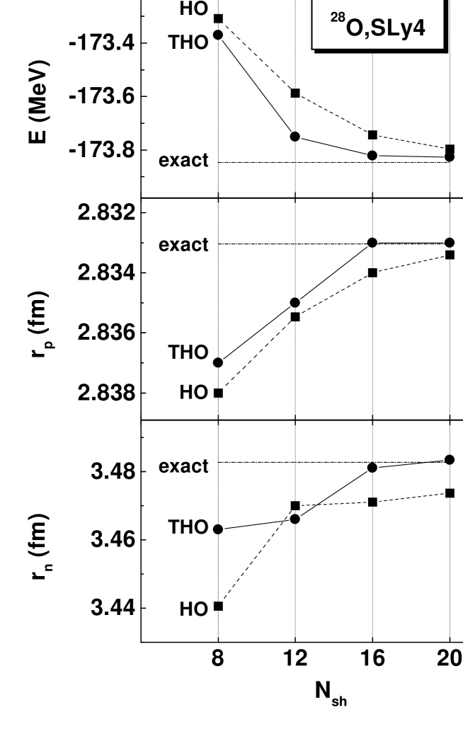
FIG. 1.: Total energies $E$, and proton and neutron rms radii, $r_{p}$ and $r_{n}$, obtained in the HFB+SLy4 calculations for ²⁸O by using the HO and THO bases, as functions of the number of HO shells $N_{\text{sh}}$. The exact results refer to those obtained from spherical coordinate-space calculations.

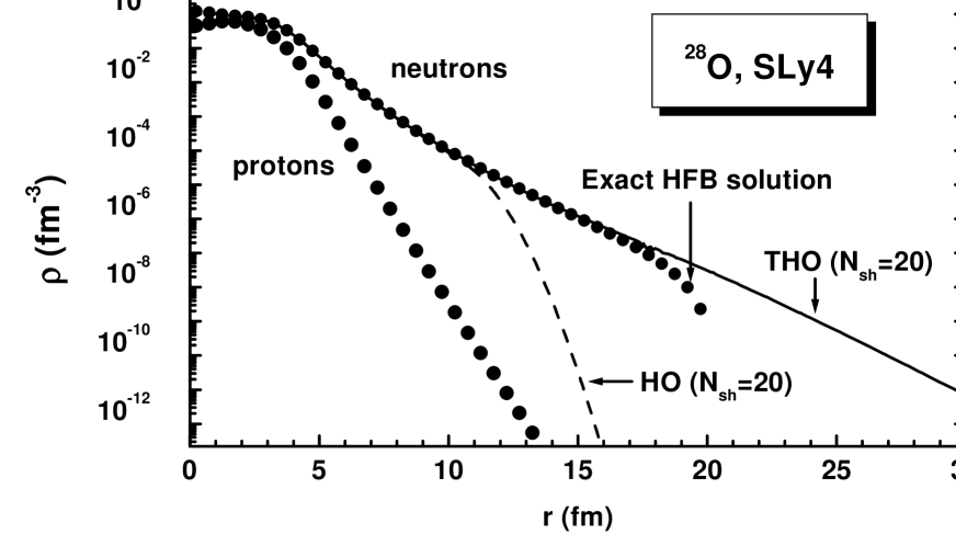
FIG. 2.: Neutron densities obtained in the HFB+SLy4 calculations for ²⁸O by using the HO (dashed line) and THO (solid line) bases. Neutron and proton densities denoted as “exact” (dots) have been obtained from spherical coordinate-space calculations in a box of $R_{\text{box}}$ =20 fm.

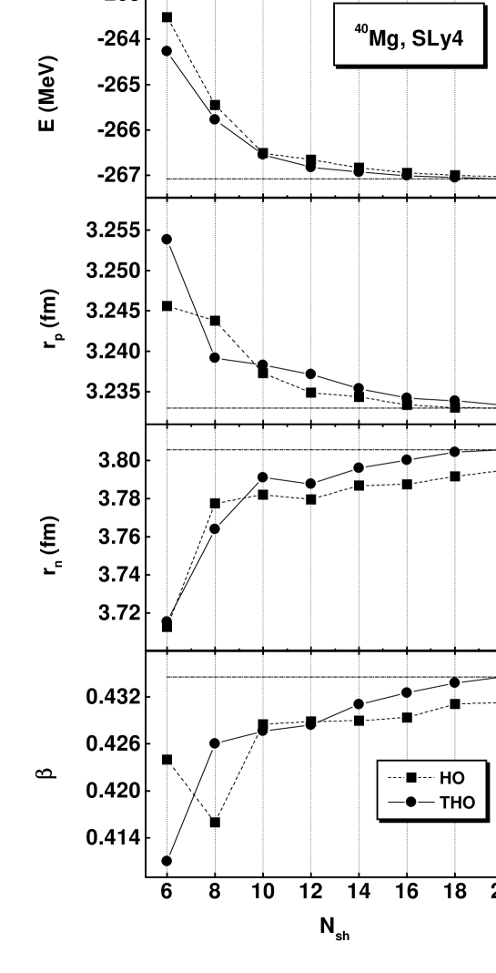
FIG. 3.: Total energies $E$, proton and neutron rms radii, $r_{p}$ and $r_{n}$, and deformations $\beta$ obtained in the HFB+SLy4 calculations for ⁴⁰Mg by using the HO and THO bases, as functions of the number of HO shells $N_{\text{sh}}$. The horizontal lines denote the THO results obtained at $N_{\text{sh}}$=20.

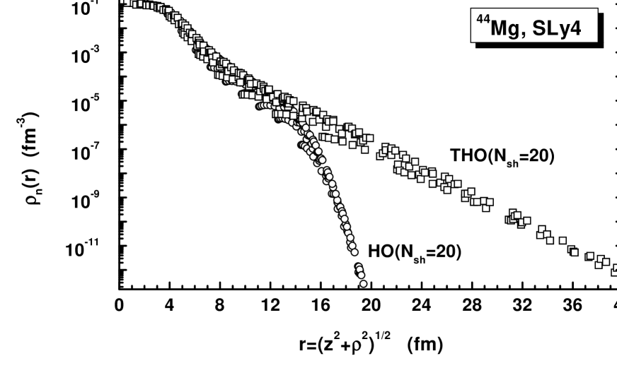
FIG. 4.: Neutron densities obtained in the HFB+SLy4 calculations for the deformed ground state of ⁴⁴Mg by using the HO (circles) and THO (squares) bases. Each point corresponds to one Gauss-integration node in the $z$-$\rho$ plane, and the results are plotted as functions of the distance from the origin, $r$=$(z^{2}$+$\rho^{2})^{1/2}$.

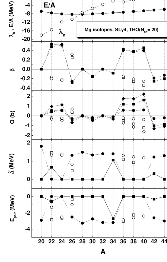
FIG. 5.: Neutron Fermi energies $\lambda_{n}$, energies per particle $E/A$, deformations $\beta$, quadrupole moments $Q$, pairing gaps $\widetilde{\Delta}$, and pairing energies $E_{\text{pair}}$ calculated for the Mg isotopes within the HFB+SLy4 method in the THO basis ($N_{\text{sh}}$=20), as functions of the mass number $A$. Apart from the upper panel, circles, squares, and diamonds pertain to proton, neutron, and total results, respectively. Closed symbols connected with lines denote values for the absolute minima in the deformation-energy curve (axial shapes are assumed), while open symbols pertain to secondary minima.

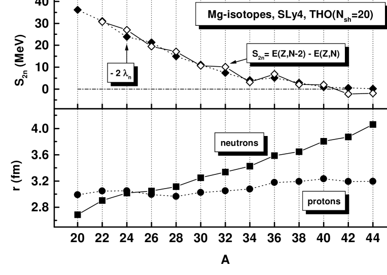
FIG. 6.: Upper panel: two-neutron separation energies $S_{2n}$ (open symbols) compared to $-2\lambda_{n}$ (closed symbols), and lower panel: proton and neutron rms radii. Calculations for the Mg isotopes were performed within the HFB+SLy4 method in the THO basis for $N_{\text{sh}}$=20.

FIG. 7.: Neutron Fermi energies $\lambda_{n}$, energies per particle $E/A$, pairing gaps $\widetilde{\Delta}$, pairing energies $E$, deformations $\beta$, quadrupole moments $Q$, and rms radii $r$ calculated for the neutron-drip-line nuclei (indicated in the lower panel) within the HFB+SLy4 method in the THO basis, as functions of the mass number $A$. Circles, squares, and diamonds pertain to proton, neutron, and total results, respectively.

- [1] E. Roeckl, Rep. Prog. Phys. 55, 1661 (1992).
- [2] A. Mueller and B. Sherril, Annu. Rev. Nucl. Part. Sci. 43, 529 (1993).
- [3] P.-G. Hansen, Nucl. Phys. A553, 89c (1993).
- [4] J. Dobaczewski and W. Nazarewicz, Phil. Trans. R. Soc. Lond. A 356, 2007 (1998).
- [5] A. Bulgac, Preprint FT-194-1980, Central Institute of Physics, Bucharest, 1980, nucl-th/9907088.
- [6] J. Dobaczewski, H. Flocard, and J. Treiner, Nucl. Phys. A422, 103 (1984).
- [7] J. Dobaczewski, W. Nazarewicz, T.R. Werner, J.-F. Berger, C.R. Chinn, and J. Dechargé, Phys. Rev. C53, 2809 (1996).
- [8] J. Terasaki, H. Flocard, P.-H. Heenen, and P. Bonche, Nucl. Phys. A621, 706 (1997).
- [9] N. Tajima, XVII RCNP International Symposium on Innovative Computational Methods in Nuclear Many-Body Problems, eds. H. Horiuchi et al. (World Scientific, Singapore, 1998) p. 343.
- [10] M.V. Stoitsov, P. Ring, D. Vretenar, and G.A. Lalazissis, Phys. Rev. C58, 2086 (1998).
- [11] M.V. Stoitsov, W. Nazarewicz, and S. Pittel, Phys. Rev. C58, 2092 (1998).
- [12] I.Zh. Petkov and M.V. Stoitsov, Compt. Rend. Bulg. Acad. Sci. 34, 1651 (1981); Theor. Math. Phys. 55, 584 (1983); Sov. J. Nucl. Phys. 37, 692 (1983).
- [13] M.V. Stoitsov and I.Zh. Petkov, Ann. Phys. (NY) 184, 121 (1988).
- [14] I.Zh. Petkov and M.V. Stoitsov, Nuclear Density Functional Theory, Oxford Studies in Physics, (Clarendon Press, Oxford, 1991).
- [15] J. Dobaczewski and J. Dudek, Comp. Phys. Commun. 102, 166 (1997); 102, 183 (1997).
- [16] D. Vautherin, Phys. Rev. C7, 296 (1973).
- [17] M. Abramowitz and I.A. Stegun, Handbook of Mathematical Functions (Dover, New York, 1970).
- [18] Y.K. Gambhir, P. Ring, and A. Thimet, Ann. Phys. (N.Y.) 198, 132 (1990).
- [19] Y.M. Engel, D.M. Brink, K. Goeke, S.J. Krieger, and D. Vautherin, Nucl. Phys. A249, 215 (1975).
- [20] P. Ring and P. Schuck, The Nuclear Many-Body Problem (Springer-Verlag, Berlin, 1980).
- [21] V.E. Oberacker and A.S. Umar, Proc. Int. Symp. on Perspectives in Nuclear Physics, (World Scientific, Singapore, 1999), Report nucl-th/9905010.
- [22] J. Terasaki, P.-H. Heenen, H. Flocard, and P. Bonche, Nucl. Phys. A600, 371 (1996).
- [23] D. Gogny, Nucl. Phys. A237, 399 (1975).
- [24] M. Girod and B. Grammaticos, Phys. Rev. C27, 2317 (1983).
- [25] J.L. Egido, H.-J. Mang, and P. Ring, Nucl. Phys. A334, 1 (1980).
- [26] J.L. Egido, J. Lessing, V. Martin, and L.M. Robledo, Nucl. Phys. A594, 70 (1995).
- [27] A.V. Afanasjev, J. König, and P. Ring, Nucl. Phys. A608, 107 (1996).
- [28] P. Ring, Prog. Part. Nucl. Phys. 37, 193 (1996).
- [29] E. Chabanat, P. Bonche, P. Haensel, J. Meyer, and F. Schaeffer, Nucl. Phys. A635, 231 (1998).
- [30] X. Li and P.-H. Heenen, Phys. Rev. C54, 1617 (1996).
- [31] S. Ćwiok, J. Dobaczewski, P.-H. Heenen, P. Magierski, and W. Nazarewicz, Nucl. Phys. A611, 211 (1996).
- [32] K. Rutz, M. Bender, T. Buervenich, T. Schilling, P.-G. Reinhard, J. A. Maruhn, and W. Greiner, Phys. Rev. C56, 238 (1997).
- [33] P.H. Heenen, J. Dobaczewski, W. Nazarewicz, P. Bonche, and T.L. Khoo, Phys. Rev. C57, 1719 (1998).
- [34] F. Naulin, J.Y. Zhang, H. Flocard, D. Vautherin, P.H. Heenen, and P. Bonche, Phys. Lett. 429B, 15 (1998).
- [35] W. Satuła, J. Dobaczewski, and W. Nazarewicz, Phys. Rev. Lett. 81, 3599 (1998).
- [36] T. Bürvenich, K. Rutz, M. Bender, P.-G. Reinhard, J.A. Maruhn, and W. Greiner, Eur. Phys. J. A3, 139 (1998).
- [37] D. Rudolph, C. Baktash, J. Dobaczewski, W. Nazarewicz, W. Satuła, M.J. Brinkman, M. Devlin, H.-Q. Jin, D.R. LaFosse, L.L. Riedinger, D.G. Sarantites, and C.-H. Yu, Phys. Rev. Lett. 80, 3018 (1998).
- [38] S. Bouneau, F. Azaiez, J. Duprat, I. Deloncle, M.G. Porquet, A. Astier, M. Bergstrom, C. Bourgeois, L. Ducroux, B.J.P. Gall, M. Kaci, Y. Le Coz, M. Meyer, E.S. Paul, N. Redon, M.A. Riley, H. Sergolle, J.F. Sharpey-Schafer, J. Timar, A.N. Wilson, and R. Wyss, Eur. Phys. Jour. A2, 245 (1998).
- [39] S. Bouneau, F. Azaiez, J. Duprat, I. Deloncle, M.G. Porquet, A. Astier, M. Bergstrom, C. Bourgeois, L. Ducroux, B.J.P. Gall, M. Kaci, Y. Le Coz, M. Meyer, E.S. Paul, N. Redon, M.A. Riley, H. Sergolle, J.F. Sharpey-Schafer, J. Timar, A.N. Wilson, R. Wyss, and P.-H. Heenen, Phys. Rev. C58, 3260 (1998).
- [40] D. Rudolph, C. Baktash, M.J. Brinkman, E. Caurier, D.J. Dean, M. Devlin, J. Dobaczewski, P.-H. Heenen, H.-Q. Jin, D.R. LaFosse, W. Nazarewicz, F. Nowacki, A. Poves, L.L. Riedinger, D.G. Sarantites, W. Satuła, and C.-H. Yu, Phys. Rev. Lett. 82, 3763 (1999).
- [41] C. Rigollet, P. Bonche, F. Flocard, and P.-H. Heenen, Phys. Rev. C59, 3120 (1999).
- [42] K. Bennaceur, J. Dobaczewski, and M. Płoszajczak, Phys. Rev. C60, 034308 (1999).
- [43] J. Dobaczewski, W. Nazarewicz, and T.R. Werner, Physica Scripta T56, 15 (1995).
- [44] O. Tarasov, R. Allatt, J.C. Angelique, R. Anne, C. Borcea, Z. Dlouhy, C. Donzaud, S. Grevy, D. Guillemaud-Mueller, M. Lewitowicz, S. Lukyanov, A.C. Mueller, F. Nowacki, Yu. Oganessian, N.A. Orr, A.N. Ostrowski, R.D. Page, Yu. Penionzhkevich, F. Pougheon, A. Reed, M.G. Saint-Laurent, W. Schwab, E. Sokol, O. Sorlin, W. Trinder, and J.S. Winfield, Phys. Lett. 409B, 64 (1997).
- [45] H. Sakurai, S.M. Lukyanov, M. Notani, N. Aoi, D. Beaumel, N. Fukuda, M. Hirai, E. Ideguchi, N. Imai, M. Ishihara, H. Iwasaki, T. Kubo, K. Kusaka, H. Kumagai, T. Nakamura, H. Ogawa, Yu.E. Penionzhkevich, T. Teranishi, Y.X. Watanabe, K. Yoneda, and A. Yoshida, Phys. Lett. 448B, 180 (1999).
- [46] A.T. Kruppa, P.-H. Heenen, H. Flocard, and R.J. Liotta, Phys. Rev. Lett. 79, 2217 (1997).
- [47] E. Caurier, F. Nowacki, A. Poves, and J. Retamosa, Phys. Rev. C58, 2033 (1998).
- [48] T. Motobayashi, Y. Ikeda, Y. Ando, K. Ieki, M. Inoue, N. Iwasa, T. Kikuchi, M. Kurokawa, S. Moriya, S. Ogawa, H. Murakami, S. Shimoura, Y. Yanagisawa, T. Nakamura, Y. Watanabe, M. Ishihara, T. Teranishi, H. Okuno, and R.F. Casten, Phys. Lett. B 346, 9 (1995).
- [49] D. Habs, O. Kester, G. Bollen, L. Liljeby, K.G. Rensfelt, D. Schwalm, R. von Hahn, G. Walter, P. Van Duppen, and the REX-ISOLDE Collaboration, Nucl. Phys. A616, 29c (1997).
- [50] F. Azaiez et al., Int. Conf. on Nuclear Structure, Gatlinburg 1998; to be published.
- [51] P.-G. Reinhard, D.J. Dean, W. Nazarewicz, J. Dobaczewski, J.A. Maruhn, and M.R. Strayer, Phys. Rev. C60, 014316 (1999).
- [52] F. Sarazin, H. Savajols, W. Mittig, P. Roussel-Chomaz, G. Auger, D. Baiborodin, A.V. Belozyorov, C. Borcea, Z. Dlouhy, A. Gillibert, A.S. Lalleman, M. Lewitowicz, S.M. Lukyanov, F. Nowacki, F. de Oliveira, N. Orr, Y.E. Penionzhkevich, Z. Ren, D. Ridikas, H. Sakuraï, O. Tarasov, and A. de Vismes, Proc. of the XXXVII Int. Winter Meeting on Nuclear Physics, ed. I. Iori (Università degli Studi di Milano, Milano, 1999) Suppl. No. 114.
- [53] I. Tanihata, J. Phys. G 24, 1311 (1998).
- [54] P. Möller, J.R. Nix, W.D. Myers, and W.J. Swiatecki, Atom. Data and Nucl. Data Tables 59, 185 (1995).
- [55] Z. Ren, Z.Y. Zhu, Y.H. Cai, and G. Xu, Phys. Lett. B 380, 241 (1996).
- [56] G.A. Lalazissis, A.R. Farhan, and M.M. Sharma, Nucl. Phys. A628, 221 (1998).
- [57] G.A. Lalazissis, D. Vretenar, P. Ring, M. Stoitsov, and L.M. Robledo, Phys. Rev. C60, 014310 (1999).
- [58] J. Dobaczewski, Acta Phys. Pol. B30, 1647 (1999).
- [59] S. Mizutori, G. Lalazissis, J. Dobaczewski, W. Nazarewicz, and P.-G. Reinhard, to be published.
- [60] G. Audi and A.H. Wapstra, Nucl. Phys. A565, 1 (1993); Nucl. Phys. A565, 66 (1993).
- [61] K. Yoneda, N. Aoi, H. Iwasaki, H. Sakurai, H. Ogawa, T. Nakamura, W.-D. Schmidt-Ott, M. Schaefer, M. Notani, N. Fukuda, E. Ideguchi, T. Kishida, S.S. Yamamoto, and M. Ishihara, J. Phys. G24, 1395 (1998).