Constraints on vector meson photoproduction spin observables

Abstract

Extraction of spin observables from vector meson photoproduction on a nucleon target is described. Starting from density matrix elements in the vector meson’s rest frame, we transform to spin observables in the photon-nucleon c.m. frame. Several constraints on the transformed density matrix and on the spin observables follow from requiring that the angular distribution and the density matrix be positive definite. A set of constraints that are required in order to extract meaningful spin observables from forthcoming data are enunciated.

I INTRODUCTION

In an earlier paper [1], we emphasized that the angular distribution of the pseudoscalar mesons that arise from the decay of photoproduced vector mesons does not depend on the vector meson’s vector polarization, but only on its tensor polarization and that standard single and double spin observables need to be defined in the overall photon-nucleon center of mass frame. It was also found that a simple description for the decay angular distribution in the $\gamma N$ c.m. frame is obtained by using the angle between the decay meson’s velocity difference vector and the direction of the photoproduced vector meson. The main purpose of this paper is to formulate a procedure for extracting meaningful spin observables from the analysis of forthcoming vector meson photoproduction data to allow one to examine conventional spin observables. These spin observables are subject to known rules concerning their forward and backward angular behavior [2]. The nodal structure of spin observables, e. g., their production angle dependence, might reveal important underlying dynamics such as baryonic and mesonic resonances.

Here we show how to extract meaningful spin observables under the assumption that analysis of the photoproduction of vector mesons will yield a vector meson rest-frame density matrix. Since new data are not yet available, we invoked older 1968 Aachen et al. information [3] and found that some of their vector meson rest-frame density matrix results, when transformed to spin observables in the photon-nucleon center of mass frame, violated basic constraints and therefore need to be rejected. The grounds for that rejection was that some of their elements, even including their stated uncertainties, yielded non-positive, and therefore unacceptable angular distribution functions. That observation, which we subsequently found to be related to a set of constraints deduced by others earlier [4, 5], led us to examine the various constraints based on the positivity of the density matrix.

In Sec. II, we analyze the limits on the tensor polarization provided by the simple requirement that the angular distribution of the decay mesons be a positive definite function. Simple limits on the tensor polarizations follow from evaluating the decay angular distribution at selected angles. In Sec. III, the limits on observables due to positivity of the density matrix are discussed. In Sec. IV, constraints on the vector meson’s density matrix due to Daboul’s analysis [4] using Schwarz inequalities, are invoked and analyzed. The Schwarz inequalities described by Daboul can be re-expressed as four separate conditions on spin observables. However, all but two of these conditions are already contained in the simple requirement that the angular distribution should be positive definite. The two remaining conditions involve not only the tensor polarization, but also the vector meson’s vector polarization. These conditions could also be used to limit the vector meson’s vector polarization. Finally, in Sec. V the method for extracting spin observables from actual data is outlined.

Use of these basic constraints should be included in the fitting procedure to assure that general requirements concerning the angular dependence of spin observables, especially at forward and back angles, are satisfied and could then be used to deduce interesting new dynamics.

II The decay distribution

In photoproduction of a vector meson ($\rho,\phi$) on a nucleon target the final vector meson decays into two pseudoscalar mesons. The angular distribution of the decay provides information about the spin-state of the vector meson. However, only information about the tensor polarizations $T^{V}_{20},T^{V}_{21},T^{V}_{22}$ can be obtained. The angular distribution of the pseudoscalar decay mesons is given by [1]:

$$\overline{W}^{V}(\bar{\theta},\bar{\phi}) = \frac{1}{4\pi}\xi_{V}(\bar{\theta})\,\,[1-\sqrt{2}\ T^{V}_{2\mu}(\Theta,\Phi)\ {\bf C}^{*}_{2\mu}(\bar{\theta}\bar{\phi})]$$ (1)

$$= \frac{1}{4\pi}\xi_{V}(\bar{\theta})\,[1-\sqrt{\frac{1}{2}}T^{V}_{20}(3\cos^{2}\bar{\theta}-1)+\sqrt{3}\ T^{V}_{21}\,\sin 2\bar{\theta}\cos\bar{\phi}-\sqrt{3}\,T^{V}_{22}\,\sin^{2}\bar{\theta}\cos 2\bar{\phi}].$$ (2)

Here ${\bf C}^{*}_{2\mu}\equiv\sqrt{\frac{4\pi}{5}}\,Y^{*}_{2\mu}$ is a spherical harmonic function and the angles $\bar{\theta},\bar{\phi}$ refer to the direction between the velocity vector difference, $\Delta\vec{v}\equiv\vec{v}_{1}-\vec{v}_{2},$ and the momentum vector of the produced vector meson; $\vec{v}_{1}$ and $\vec{v}_{2}$ refer to the velocity vectors of the two decay mesons in the overall photon-nucleon center of mass frame. Use of these angles simplifies the expression for the angular distribution in the overall photon-nucleon center of mass frame in which spin observables are defined. Note that the spin observables $T^{V}_{2\mu}$ depend on the vector meson production angles $\Theta,\Phi,$ as well as on the total c.m. energy. The factor $\xi,$ which arises from describing the vector meson decay in the overall center of mass system and from a density of state factor, is given by:

$$\xi_{V}(\bar{\theta})=\frac{1}{(\sin^{2}\bar{\theta}+(\frac{E_{\rho}}{m_{\rho}})^{2}\cos^{2}\bar{\theta})^{5/2}}\ \ ,$$ (3)

where $m_{\rho},E_{\rho}$ are the vector meson’s mass and energy.

The decay angular distribution $\overline{W}^{V}(\bar{\theta},\bar{\phi})$ does not depend on the vector meson’s vector polarization and as shown above includes only the vector meson’s tensor polarization. Once the angular distribution is measured and vector meson rest frame density matrices are provided, it is necessary to map that data over to the angles $\bar{\theta},\bar{\phi}.$ One can then project out the vector meson’s tensor polarization from the normalized ratio $\overline{W}^{V}_{norm}(\bar{\theta},\bar{\phi})\equiv\overline{W}^{V}(\bar{\theta},\bar{\phi})/\xi,$ as described in Sec. V.

The tensor polarization must take on values that allow the angular distribution function $\overline{W}^{V}(\bar{\theta},\bar{\phi})$ to be positive definite. By selecting the angles $\bar{\theta},\bar{\phi}$ one can use that obvious condition to extract allowed limits for the tensor polarization. In the first and second columns of Table I a list is given of specific choices of angles $\bar{\theta},\bar{\phi}$ and the resulting conditions on $T^{V}_{20},T^{V}_{21},T^{V}_{22}.$ Such constraints also arise from direct conditions on the density matrix, as will be seen in Sections III and IV.

Thus from Table I, we see that the simple requirement that the decay angular cross section be positive yields limits on the possible tensor polarization. We now consider other ways to recognize constraints on the spin observables and the associated density matrix. In the next section, we describe the constraints on $T^{V}_{20},T^{V}_{21},T^{V}_{22}$ that follow from the positivity of the density matrix.

III Limits on observables for a positive definite density matrix

Recall that for a general observable $\Omega$ the classical ensemble average is

$$<\Omega>=\frac{\sum_{\alpha}\omega_{\alpha}<\alpha\,|\Omega|\,\alpha>}{\sum_{\alpha}\omega_{\alpha}},$$ (4)

where $\omega_{\alpha}$ is the positive definite probability for finding a beam particle pointing in the direction stipulated by the Euler angle label $\alpha.$ Note that the above is a classical average, with the quantum effects isolated into the expectation value for each beam particle $<\,\alpha|\Omega|\,\alpha>.$

The spin density matrix of the vector meson is defined as

$$\rho=\sum_{\alpha}\ |\,\alpha\,>\omega_{\alpha}<\,\alpha\,|\ ,$$ (5)

where $\omega_{\alpha}$ is non-negative. The helicity matrix elements of the density matrix are

$$\rho_{\lambda\lambda^{\prime}}=\sum_{\alpha}\ <\lambda\,|\,\alpha>\omega_{\alpha}<\alpha\,|\,\lambda^{\prime}>.$$ (6)

The classical ensemble average for observable $\Omega$ is now obtained from the density matrix $\rho$ as

$$<\Omega>=\frac{Tr[\rho\Omega]}{Tr[\rho]}.$$ (7)

The density matrix $\rho$ is positive definite, which can be shown as follows. Let us define [4] a set of vectors $v_{\lambda}$ by its elements in $\alpha$ space

$$v_{\lambda}^{\alpha}\equiv<\alpha|\lambda>\sqrt{\omega_{\alpha}}\ .$$ (8)

The elements $\rho_{\lambda\lambda^{\prime}}$ of the density matrix can now be written as dot-products in $\alpha$ space of the set of vectors $v_{\lambda}$  ,

$$\rho_{\lambda\lambda^{\prime}}=(v_{\lambda},v_{\lambda^{\prime}}).$$ (9)

Now for any vector $X$

$$X^{\dagger}\rho X=\sum_{\lambda,\lambda^{\prime}}\ X^{*}_{\lambda}\rho_{\lambda\lambda^{\prime}}X_{\lambda^{\prime}}=(\sum_{\lambda}X_{\lambda}v_{\lambda},\sum_{\lambda^{\prime}}X_{\lambda^{\prime}}v_{\lambda^{\prime}})\geq 0,$$ (10)

which displays the positive definiteness of $\rho$.

At this point we explore the linear constraints on the matrix elements of $\rho$ implied by Eq. (10). The density matrix $\rho$ is a $3\times 3$ matrix with elements $\rho_{\lambda,\lambda^{\prime}}$ where the helicity $\lambda$ takes the values $1,0,-1.$ Since the production of the vector meson occurs via a parity conserving mechanism, the spin density matrix elements satisfy the symmetries

$$\rho_{\lambda\lambda^{\prime}}=\rho^{*}_{\lambda^{\prime}\lambda},\ \ \ \ \ {\rm and}\ \ \ \ \ \rho_{\lambda\lambda^{\prime}}=(-1)^{\lambda-\lambda^{\prime}}\rho_{-\lambda-\lambda^{\prime}}.$$ (11)

The density matrix takes the form

$$\rho=\left(\begin{array}[]{ccc}(1-\rho_{00})/2&\Re\rho_{10}+i\Im\rho_{10}&\rho_{1-1}\\ \Re\rho_{10}-i\Im\rho_{10}&\rho_{00}&-\Re\rho_{10}+i\Im\rho_{10}\\ \rho_{1-1}&-\Re\rho_{10}-i\Im\rho_{10}&(1-\rho_{00})/2\end{array}\right).$$ (15)

In the language of spin observables $P^{V}_{y},T^{V}_{20},T^{V}_{21},T^{V}_{22}$ the density matrix can be written as

$$\rho=\frac{1}{3}[I+\frac{3}{2}\vec{S}\cdot\vec{P}^{V}+\tau\cdot T^{V}],$$ (16)

where $\vec{S}$ is the spin-1 operator and $\tau$ is the symmetric traceless rank-2 operator with cartesian components $\tau_{ij}=\frac{3}{2}(S_{i}S_{j}+S_{j}S_{i})-2\delta_{ij}$. In matrix form this becomes

$$\rho=\frac{1}{3}\left(\begin{array}[]{ccc}1+\sqrt{\frac{1}{2}}T^{V}_{20}&\frac{3}{2}\sqrt{\frac{1}{2}}(-iP^{V}_{y})-\sqrt{\frac{3}{2}}T^{V}_{21}&\sqrt{3}\ T^{V}_{22}\\ \frac{3}{2}\sqrt{\frac{1}{2}}(iP^{V}_{y})-\sqrt{\frac{3}{2}}T^{V}_{21}&1-\sqrt{2}\ T^{V}_{20}&\frac{3}{2}\sqrt{\frac{1}{2}}(-iP^{V}_{y})+\sqrt{\frac{3}{2}}T^{V}_{21}\\ \sqrt{3}\ T^{V}_{22}&\frac{3}{2}\sqrt{\frac{1}{2}}(iP^{V}_{y})+\sqrt{\frac{3}{2}}T^{V}_{21}&1+\sqrt{\frac{1}{2}}T^{V}_{20}\end{array}\right).$$ (20)

If the vector $X$ in Eq. (10) is such that the combination $X^{*}_{\lambda}X_{\lambda^{\prime}}$ is symmetric under the exchange of $\lambda$ and $\lambda^{\prime},$ the obtained constraints are similar to the constraints derived in the previous section for a positive decay angular distribution. The constraints in that case involve only the tensor polarizations $T^{V}_{20},T^{V}_{21},$ and $T^{V}_{22}$, and not the vector polarization $P^{V}_{y}$. This is because symmetric combinations $X^{*}_{\lambda}X_{\lambda^{\prime}}$ only pick out the symmetric part of the density matrix $\rho_{\lambda\lambda^{\prime}}$, i. e., in this case the part that has even rank. The antisymmetric rank-one part of $\rho$, which is due to the vector polarization, then gives no contribution to $X^{\dagger}\rho X$. This is exactly the symmetry selection made if one considers the decay angular distribution of Section II, and which was discussed in detail in Ref. [1]. The resultant linear constraints are listed in columns 1 and 3 of Table I.

Even relations involving the vector polarization $P^{V}_{y}$ can be obtained from Eq. (10), if the above symmetry restrictions are not invoked on $X^{*}_{\lambda}X_{\lambda^{\prime}}$. However, the resulting linear constraints involving $P^{V}_{y}$ are only of academic interest because $P^{V}_{y}$ cannot be measured from the decay angular distribution. These additional constraints are therefore not listed in this paper.

IV Spin observable limits from Schwarz inequalities

Additional constraints on the density matrix are obtained using Schwarz inequalities as described in Ref. [4]. Namely, from the previously derived Eq. (9) and

$$|(v_{\lambda},v_{\lambda^{\prime}})|\leq|v_{\lambda}||v_{\lambda^{\prime}}|\ ,$$ (21)

follows

$$|\rho_{\lambda\lambda^{\prime}}|\leq\sqrt{\rho_{\lambda\lambda}\ \rho_{\lambda^{\prime}\lambda^{\prime}}}\ \ .$$ (22)

Similar constraints exist for differences or sums of matrix elements $\rho_{\lambda\lambda^{\prime}}$. Such constraints were exploited in Ref. [4]. In this case, two additional inequalities can be derived

$$|\rho_{\lambda\lambda^{\prime}}+\rho_{-\lambda\lambda^{\prime}}|\leq\sqrt{2(\rho_{\lambda\lambda}+\rho_{\lambda-\lambda})\ \rho_{\lambda^{\prime}\lambda^{\prime}}},$$ (23)

and

$$|\rho_{\lambda\lambda^{\prime}}-\rho_{-\lambda\lambda^{\prime}}|\leq\sqrt{2(\rho_{\lambda\lambda}-\rho_{\lambda-\lambda})\ \rho_{\lambda^{\prime}\lambda^{\prime}}}.$$ (24)

From Eqs. (22,23,24) one finds several quadratic constraints. Using Eq. (11) and the property that the diagonal matrix elements $\rho_{1,1},\rho_{0,0}$, and $\rho_{-1,-1}$ are non-negative or

$$1+\sqrt{\frac{1}{2}}\ T^{V}_{20}\geq 0,$$ (25)

$$1-\sqrt{2}\ T^{V}_{20}\geq 0,$$ (26)

some of the Schwarz inequalities collapse to linear conditions

$$1+\sqrt{\frac{1}{2}}T^{V}_{20}+\sqrt{3}T^{V}_{22}\geq 0,$$ (27)

$$1+\sqrt{\frac{1}{2}}T^{V}_{20}-\sqrt{3}T^{V}_{22}\geq 0.$$ (28)

However, one also finds two very useful quadratic conditions that involve the squares of $P^{V}_{y}$ and $T^{V}_{21},$

$$9(P^{V}_{y})^{2}+12(T^{V}_{21})^{2}\leq 8(1-\sqrt{2}T^{V}_{20})(1+\sqrt{\frac{1}{2}}T^{V}_{20}),$$ (29)

$$9(P^{V}_{y})^{2}+12(T^{V}_{21})^{2}\leq 4(1-\sqrt{2}T^{V}_{20})(1+\sqrt{\frac{1}{2}}T^{V}_{20}-\sqrt{3}T^{V}_{22}).$$ (30)

The resulting restrictions on the observables are listed in columns 1 and 4 of Table I and Table II. As one can see, the obtained linear rules are equivalent to those discussed earlier. Again we omit from Table I linear conditions that include $P^{V}_{y}$.

V Data Analysis Method

The Aachen et al. [3] collaboration measured the reaction $\gamma+p\rightarrow\rho^{0}+p$ using an unpolarized photon beam and an unpolarized proton target. The final proton recoils when a $\rho$ meson is produced and the $\rho$ subsequently decays into $\pi^{+}$ and $\pi^{-}$ mesons, both of which are detected. Hence, the angular pion distribution in the final state is measured. A fit to this angular distribution in the $\rho$ meson rest-frame yields three density matrix elements from which we can reconstruct their pion angular distribution in the $\rho$ meson rest frame. This reconstructed decay pion angular distribution is called $W^{V}(\theta,\phi)$, where $\theta,\phi$ define the direction of $\pi^{+}$ in the $\rho$ rest frame.

The above pion angular distribution depends on the spin state of the produced $\rho$ meson, which is described by a $3\times 3$ spin density matrix $\rho_{\lambda,\lambda^{\prime}}$. The angular distribution only depends on the three real elements $\rho_{00}$, $\Re\rho_{10}$, $\rho_{1-1}$. Values of these elements in the rest frame of the $\rho$ meson are published by Aachen et al. [3] for a set of several photon beam energies and vector meson production angles. In order to study reaction mechanisms, however, we are interested in spin correlations(single and double spin observables) that are defined in the overall center of mass frame. How does one obtain spin correlations from these previously published density matrix elements?

Our aim is to use the Aachen et al. data in the form of $W^{V}(\theta,\phi)$ to obtain the pion angular distribution in the photon-nucleon center of mass frame and re-analyze it in terms of the spin correlations. If one or more particles in the reaction are polarized [1], such future data can be analyzed in a similar way to extract meaningful spin correlations. Our procedure is therefore preparation for analysis of future experimental results from Thomas Jefferson Laboratory with polarized photons [7].

The first step is to obtain the angular distribution $W^{V}(\theta,\phi)$ in the $\rho$ meson rest frame from the values of the elements $\rho_{00}$, $\Re\rho_{10}$, $\rho_{1-1}$ using

$$W^{V}(\theta,\phi) = \frac{3}{4\pi}[\frac{1-\,\rho_{00}}{2}+\frac{3\rho_{00}-1}{2}\cos^{2}\theta-\sqrt{2}\,\Re\rho_{10}\sin 2\theta\cos\phi-\rho_{1-1}\sin^{2}\theta\cos 2\phi]\ .$$ (31)

Then one constructs the angular distribution $\overline{W}^{V}(\bar{\theta},\bar{\phi})$ in the $\gamma$-nucleon center of mass using

$$\overline{W}^{V}(\bar{\theta},\bar{\phi}) = \frac{1}{(\sin^{2}\bar{\theta}+(\frac{E_{\rho}}{m_{\rho}})^{2}\cos^{2}\bar{\theta})^{3/2}}W^{V}(\theta(\bar{\theta}),\phi)\ .$$ (32)

In the c.m. frame the variables are $\bar{\theta}$ and $\bar{\phi}$, where $\bar{\theta},\bar{\phi}$ are the angles between the relative velocity of the two decay pions in the $\gamma$-nucleon c.m. frame. These angles are related to the angles of the decay meson in the vector meson’s rest frame by:

$$\bar{\theta}=\arctan(\frac{E_{\rho}}{m_{\rho}}\tan\theta),$$ (33)

and $\bar{\phi}=\phi.$

The next step involves including the known kinematic factor $\xi(\bar{\theta})$ in $\overline{W}^{V}(\bar{\theta},\phi)$ see Eq. (3). Aside from the overall factor of $\xi(\bar{\theta})$, the remaining angular behavior is expressed as a series in spherical harmonics:

$$\overline{W}^{V}(\bar{\theta},\bar{\phi}) = \frac{1}{4\pi}\xi(\bar{\theta})[(1-\sqrt{\frac{1}{2}}\,T^{V}_{20}(3\cos^{2}\bar{\theta}-1)+\sqrt{3}\,\ T^{V}_{21}\sin 2\bar{\theta}\cos\bar{\phi}-\sqrt{3}\,\ T^{V}_{22}\sin^{2}\bar{\theta}\cos 2\bar{\phi}].$$ (34)

Next we define $\overline{W}^{V}_{norm}(\bar{\theta},\phi)$ using Eq. (34) and $\overline{W}^{V}(\bar{\theta},\phi)\equiv\xi(\bar{\theta})\times\overline{W}^{V}_{norm}(\bar{\theta},\phi).$

Finally, we project out the three spin observables, i. e., the three tensor polarizations of the vector meson, $T^{V}_{20},T^{V}_{21},T^{V}_{22}$, from $\overline{W}^{V}_{norm}(\bar{\theta},\phi)$ using spherical harmonics $Y_{lm}(\bar{\theta},\phi)$’s. These spin observables can then be studied as function of photon energy and the vector meson production angles $\Theta,\Phi.$

Once the spin observables are properly defined and have correct production angle dependence, one can visualize the role of the tensor polarization in 3D displays of the decay angular distribution. Examples are given in Fig. 4 for the case of $\Theta=0^{\circ},180^{\circ}$ and positive $T_{20}$ and in Fig. 5 for the case of $\Theta=0^{\circ},180^{\circ}$ and negative $T_{20};$ with in both cases $T_{21}=T_{22}=0.$ In Fig. 6, a more realistic case, based on Ref. [3] for $E_{\gamma}=3GeV$ and $\Theta=70^{\circ}$ is shown; namely, for $T_{20}=-.72,T_{21}=-.21,T_{22}=.19.$ One can therefore associate a shape of $\overline{W}$ with each point in the allowed $T_{20},T_{21},T_{22}$ space.

In the process of carrying out these steps, we found four cases of the Aachen data that do not satisfy the constraints in Tables I and II. Therefore those sets had to be rejected. Subsequently we found another author had also rejected some of the data [4] using similar general constraints.

It would therefore be best to incorporate these constraints directly into the data analysis.

VI CONCLUSION

For analysis of experimental data for vector meson photoproduction one should describe the resulting angular decay distribution in the overall $\gamma N$ c.m. frame instead of in the commonly used vector-meson rest frame. In the c.m. frame, one should use the angles $\bar{\theta},\bar{\phi}$ of the relative velocity vector $\Delta\vec{v}=\vec{v}_{1}-\vec{v}_{2}$. In the transformation from the vector-meson rest frame to the $\gamma N$ c.m. frame, and due to the use of the angles $\bar{\theta},\bar{\phi},$ a kinematical factor $\xi$ of Eq. (3) needs to be included. Furthermore, constraints should be satisfied by the observables $T^{V}_{20},T^{V}_{21},T^{V}_{22}$. All of these constraints can be derived from the positivity of the density matrix.

We have also explored restrictions which follow from positivity of the eigenvalues of the spin density matrix $\rho$ such as the conditions that $\det\rho\geq 0$ and Trace$[\rho^{2}]\leq 1$, see Ref. [5]. The relations obtained from these restrictions are respectively cubic and quadratic in the spin observables and involve the vector meson’s vector polarization $P^{V}_{y}$. A more complete set of relations can be obtained by exploring the explicit forms of the roots $x_{1},x_{2},x_{3}$ of the eigenvalue equation of $\rho.$ We impose the conditions that $0\leq x_{i}\leq 1,$ $x_{1}+x_{2}+x_{3}=1,$ and $x^{2}_{1}+x^{2}_{2}+x^{2}_{3}\leq 1.$ For example, one root is $x_{1}=\frac{1}{3}(1+\frac{1}{\sqrt{2}}T^{V}_{20}+\sqrt{3}T^{V}_{22})$. From $0\leq x_{1}\leq 1$ relations follow that are similar to the rules in Table I. The other two roots are $x_{2}=\frac{1}{3}(1-\frac{1}{2\sqrt{2}}T^{V}_{20}-\frac{\sqrt{3}}{2}T^{V}_{22})-\frac{1}{2}\sqrt{P_{y}^{2}+\frac{4}{3}T_{21}^{2}+(\frac{1}{\sqrt{2}}T_{20}-\frac{1}{\sqrt{3}}T_{22})^{2}}$ and $x_{3}=1-x_{1}-x_{2}$. Both $x_{2}$ and $x_{3}$ involve $P^{V}_{y}$ and the above root rules lead to quadratic constraints that are included in Table II.

The linear and quadratic constraints on $T^{V}_{20},T^{V}_{21},T^{V}_{22}$ mean that the allowed domain in the 3-dimensional $T^{V}_{20}-T^{V}_{21}-T^{V}_{22}$ space is confined. As examples Figs. (1-3) show the allowed areas for the 2-dimensional subspaces $T^{V}_{20}-T^{V}_{21}$ , $T^{V}_{20}-T^{V}_{22}$ , and $T^{V}_{22}-T^{V}_{21}$ respectively. The dashed lines indicate the various upper bounds and the solid lines represent the lower bounds associated with the various constraints. The allowed regions are shaded. Figs. (1-3) refer in each case to 2-dimensional subspaces and only those constraints are shown that are independent of the values of the observable that would play the role of the third dimension. The full 3-dimensional representation of constraints is richer.

We close with some remarks about double spin observables. For a polarized photon beam again the angular distribution of the decay mesons can be measured. This decay distribution now depends on the single spin observables $T^{V}_{20},T^{V}_{21},T^{V}_{22}$ as well as on the double spin correlations $C^{\gamma V}_{x20},C^{\gamma V}_{x21},C^{\gamma V}_{x22},C^{\gamma V}_{y21},C^{\gamma V}_{y22},C^{\gamma V}_{z21},C^{\gamma V}_{z22}$ (Ref. [1]). (Again the vector polarization and correlations with the vector polarization cannot be measured.) Similar to the method described in Sections II and III and based on positive decay angular distributions and positivity of the complete density matrix for this case, linear and quadratic relations involving double spin observables can be derived.

The constraints on the spin observables presented in this paper should be incorporated directly into the analysis of forthcoming data.

Constraints	$W\geq 0$	$X^{\dagger}\rho X\geq 0$	Schwarz
$1-\sqrt{2}T_{20}\geq 0$	$\bar{\theta}=0$	$\rho_{00}\geq 0$	$\rho_{00}\geq 0$
$1+\frac{1}{\sqrt{2}}T_{20}\geq 0$	$\bar{\theta}=\frac{\pi}{2};\bar{\phi}=\frac{\pi}{4}$	$\rho_{11}\geq 0$	$\rho_{11}\geq 0$
$1+\frac{2}{\sqrt{3}}T_{21}\geq 0$	$\bar{\theta}=\bar{\theta}_{c};\bar{\phi}=\frac{\pi}{4}$	$1-2\sqrt{2}\Re\rho_{10}\geq 0$
$1-\frac{2}{\sqrt{3}}T_{21}\geq 0$	$\bar{\theta}=\bar{\theta}_{c};\bar{\phi}=\frac{3\pi}{4}$	$1+2\sqrt{2}\Re\rho_{10}\geq 0$
$1+\frac{2}{\sqrt{3}}T_{22}\geq 0$	$\bar{\theta}=\bar{\theta}_{c};\bar{\phi}=\frac{\pi}{2}$	$1+2\rho_{1-1}\geq 0$
$1+\frac{1}{\sqrt{2}}T_{20}+\sqrt{3}T_{22}\geq 0$	$\bar{\theta}=\frac{\pi}{2};\bar{\phi}=\frac{\pi}{2}$	$1-\rho_{00}+2\rho_{1-1}\geq 0$	$|\rho_{1-1}|^{2}\leq\rho_{11}\rho_{-1-1}$
$1+\frac{1}{\sqrt{2}}T_{20}-\sqrt{3}T_{22}\geq 0$	$\bar{\theta}=\frac{\pi}{2};\bar{\phi}=0$	$1-\rho_{00}-2\rho_{1-1}\geq 0$	$|\rho_{1-1}|^{2}\leq\rho_{11}\rho_{-1-1}$
$2-\frac{1}{\sqrt{2}}T_{20}-\sqrt{3}T_{22}\geq 0$			see caption(*)
$2-\frac{1}{\sqrt{2}}T_{20}+\sqrt{3}T_{22}\geq 0$	$\bar{\theta}=\frac{\pi}{4};\bar{\phi}=\frac{\pi}{2}$
$1-\frac{1}{2\sqrt{2}}T_{20}+\sqrt{\frac{3}{2}}T_{21}\geq 0$	$\bar{\theta}=\frac{\pi}{4};\bar{\phi}=\frac{\pi}{4}$	$1+\rho_{00}-4\Re\rho_{10}\geq 0$
$1-\frac{1}{2\sqrt{2}}T_{20}-\sqrt{\frac{3}{2}}T_{21}\geq 0$	$\bar{\theta}=\frac{3\pi}{4};\bar{\phi}=\frac{\pi}{4}$	$1+\rho_{00}+4\Re\rho_{10}\geq 0$
$1+\frac{2\sqrt{2}}{\sqrt{3}}T_{21}-\frac{2}{\sqrt{3}}T_{22}\geq 0$	$\bar{\theta}=\bar{\theta}_{c};\bar{\phi}=0$	$1-4\Re\rho_{10}-2\rho_{1-1}\geq 0$
$1-\frac{2\sqrt{2}}{\sqrt{3}}T_{21}-\frac{2}{\sqrt{3}}T_{22}\geq 0$	$\bar{\theta}=\bar{\theta}_{c};\bar{\phi}=\pi$	$1+4\Re\rho_{10}-2\rho_{1-1}\geq 0$

TABLE I.: Linear Constraints for $T_{20},T_{21},T_{22}$; $\bar{\theta}_{c}=\arccos(\frac{1}{\sqrt{3}})$. (*) This condition follows from $x_{1}\leq 1.$

Constraints	Schwarz Inequality	Other
$9P_{y}^{2}+12T_{21}^{2}\leq 8(1-\sqrt{2}T_{20})(1+\frac{1}{\sqrt{2}}T_{20})$	$|\rho_{10}|^{2}\leq\rho_{11}\rho_{00}$
$9P_{y}^{2}+12T_{21}^{2}\leq 4(1-\sqrt{2}T_{20})(1+\frac{1}{\sqrt{2}}T_{20}-\sqrt{3}T_{22})$	$|\rho_{10}-\rho_{-10}|^{2}\leq 2|\rho_{11}-\rho_{1-1}|\rho_{00}$	$x_{2}\geq 0$
$9P_{y}^{2}+12T_{21}^{2}\leq 8(1+\frac{1}{\sqrt{2}}T_{20})(2-\frac{1}{\sqrt{2}}T_{20}+\sqrt{3}T_{22})$		$x_{3}\leq 1$
$9P_{y}^{2}+12T_{21}^{2}+12T_{22}^{2}+6T_{20}^{2}\leq 12$		$Tr[\,\rho^{2}\,]\leq 1$

TABLE II.: Quadratic constraints for $P_{y},T_{20},T_{21},T_{22}$

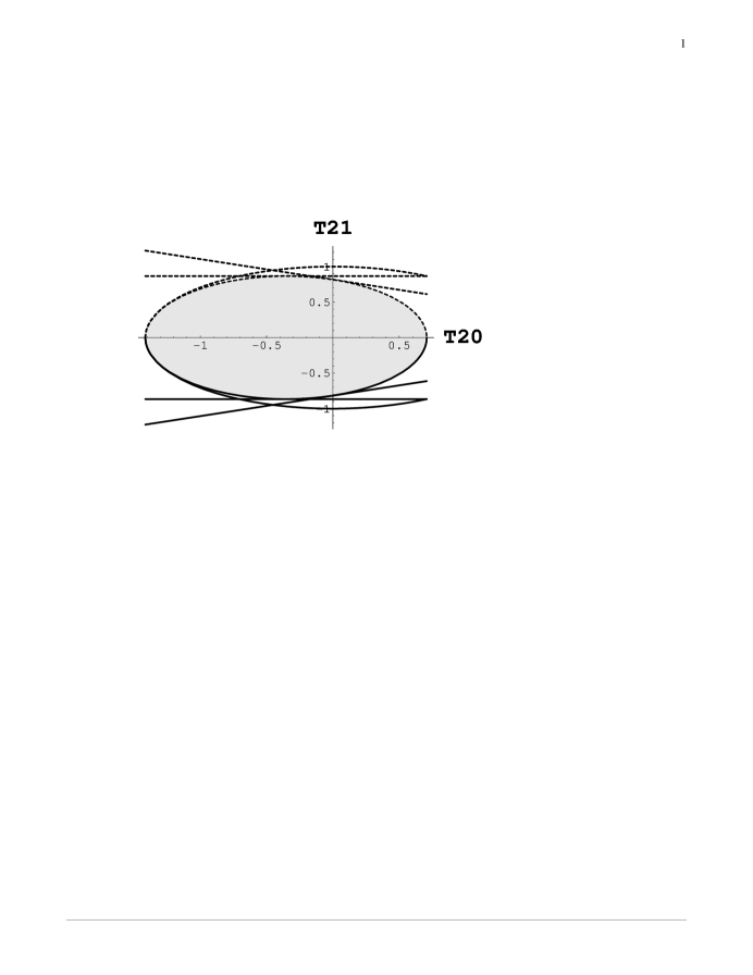
FIG. 1.: Allowed domain in the space spanned by $T^{V}_{20}$ and $T^{V}_{21}$ independent of the value of $T^{V}_{22}$. Dashed lines are upper bounds. Solid lines are lower bounds. Linear constraints are from Table 1 and quadratic constraints are from Table II. The shaded area represents the allowed region.

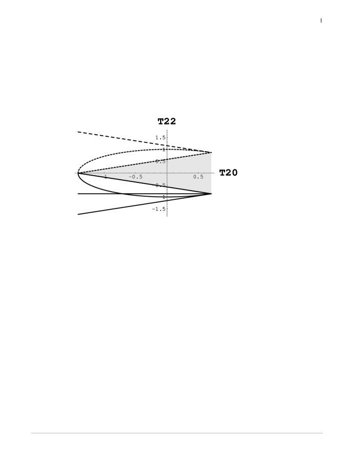
FIG. 2.: Allowed domain in the space spanned by $T^{V}_{20}$ and $T^{V}_{22}$ independent of the value of $T^{V}_{21}$. Dashed lines are upper bounds. Solid lines are lower bounds. Linear constraints are from Table 1 and quadratic constraints are from Table II. The shaded area represents the allowed region.

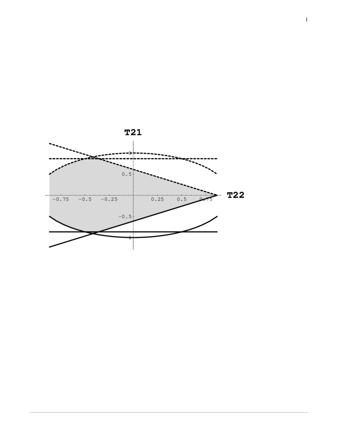
FIG. 3.: Allowed domain in the space spanned by $T^{V}_{22}$ and $T^{V}_{21}$ independent of the value of $T^{V}_{20}$. Dashed lines are upper bounds. Solid lines are lower bounds. Linear constraints are from Table 1 and quadratic constraints are from Table II. The shaded area represents the allowed region.

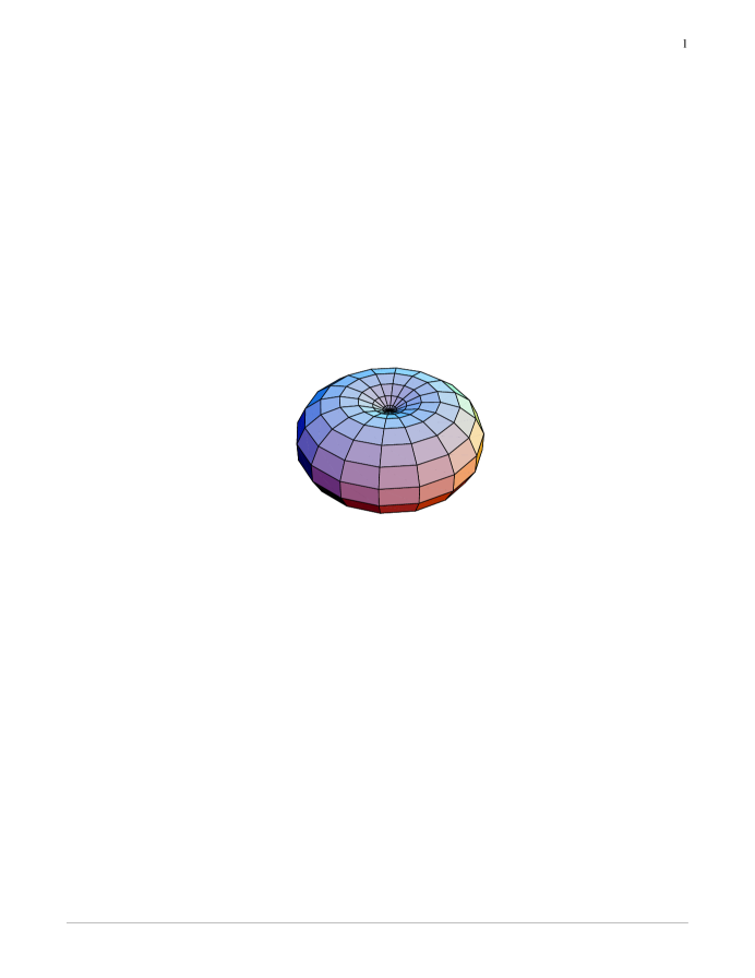
FIG. 4.: Forward/Back $\overline{W}$ for $T_{20}>0.$ This is the distribution in terms of the angles $\bar{\theta},\bar{\phi}$ with the up direction being the direction of the produced vector meson’s momentum.

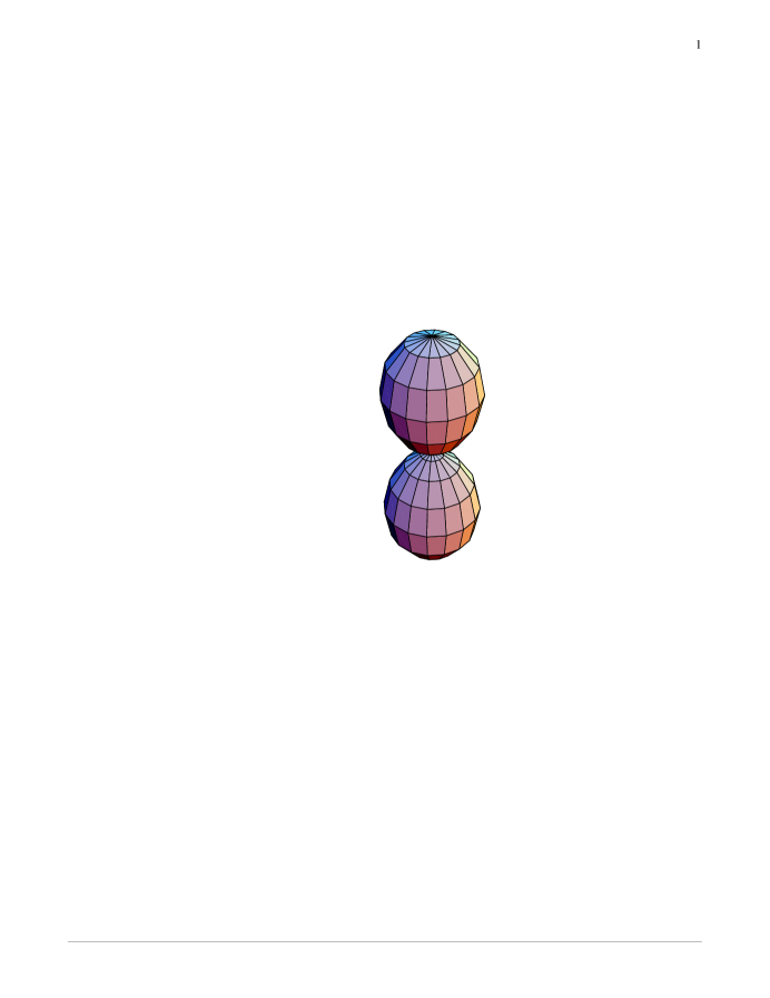
FIG. 5.: Forward/Back $\overline{W}$ for $T_{20}<0.$ This is the distribution in terms of the angles $\bar{\theta},\bar{\phi}$ with the up direction being the direction of the produced vector meson’s momentum.

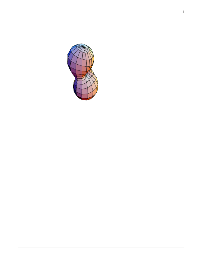
FIG. 6.: Shape of $\overline{W}$ for $T_{20}=-.72,T_{21}=-.21,T_{22}=.19.$ This is the distribution in terms of the angles $\bar{\theta},\bar{\phi}$ with the up direction being the direction of the produced vector meson’s momentum.

REFERENCES

• [1] W. M.  Kloet. Wen-tai Chiang and F. Tabakin, Phys. Rev. C 58, 1086 (1998).
• [2] M. Pichowsky, C. Savkli, and F. Tabakin, Phys. Rev. C 53 , 593 (1996).
• [3] Aachen-Berlin-Bonn-Hamburg-Heidelberg-Munchen Collaboration, Phys. Rev. 175, 1669 (1968).
• [4] J. Daboul, Nucl. Phys. B 4, 180 (1967).
• [5] P. Minnaert, Phys. Rev. 151, 1306 (1966).
• [6] Wen-tai Chiang and F. Tabakin, Phys. Rev. C , (199).
• [7] E-94-109 P. Cole, R. Whitney, and J. Connelly, Photoproduction of the Rho Meson from the Proton with Linearly Polarized Photons; E-98-109 D. Tedeschi, P. Cole, and J. Mueller, Photoproduction of phi Mesons with Linearly Polarized Photons; E-93-031 C. Marchand, M. Anghinolfi, and J. Laget, Photoproduction of Vector Mesons at High t; E-93-033 J. Napolitano and D. Weygand, A Search for Missing Baryons Formed in $\gamma P\rightarrow P\pi^{+}\pi^{-}$ Using the CLAS at CEBAF.