[

Hartree–Fock Approximation for Inverse Many–Body Problems

Abstract

A new method is presented to reconstruct the potential of a quantum mechanical many–body system from observational data, combining a nonparametric Bayesian approach with a Hartree–Fock approximation. A priori information is implemented as a stochastic process, defined on the space of potentials. The method is computationally feasible and provides a general framework to treat inverse problems for quantum mechanical many–body systems.

]

The reconstruction of inter–particle forces from observational data is of key importance for any application of quantum mechanics to real world systems. Such inverse problems have been studied intensively in inverse scattering theory and in inverse spectral theory for one–body systems in one and, later, in three dimensions [1, 2]. In this Paper we now outline a method, designed to deal with inverse problems for many–body systems.

Being the mathematical counterpart of induction problems in philosophy, inverse problems appear quite naturally in science when justification of a physical law has to be based on a finite number of observations. Such problems are notoriously ill–posed in the sense of Hadamard [3, 4]. In that case it is well known that additional a priori information is required to obtain a stable and unique solution. Referring to a Bayesian framework [5, 6, 7], we implement a priori information in form of stochastic processes over potentials [8]. While a standard procedure is to fit parameterized potentials to the data, we will especially be interested in less restrictive, nonparametric approaches. As, up to now, calculating an exact solution of inverse many–body problems is not feasible, we will treat the problem in an ‘inverse Hartree–Fock approximation’ (IHFA).

A main advantage of Bayesian methods is their flexibility. They can easily be adapted to different learning situations and have therefore been applied to a variety of empirical learning problems, including classification, regression, density estimation [9, 10], and, recently, to quantum statistics [8]. In particular, within a Bayesian approach it is straightforward to deal with measurements of arbitrary quantum mechanical observables, to include classical noise processes, and to implement a priori information explicitly in terms of the potential. Computationally, on the other hand, working with stochastic processes, or discretized versions thereof, is much more demanding than, for example, fitting parameters. This holds especially for applications to quantum mechanics where one can not take full advantage of the convenient analytical features of Gaussian processes. Due to increasing computational resources, however, the corresponding learning algorithms become now numerically feasible.

We will consider many–fermion systems with Hamiltonians, $H$ = $T+V$, consisting of a one–body part $T$, e.g., $T$ = $-(1/2m)\Delta$ (with Laplacian $\Delta$, mass $m$, $\hbar$ = 1), and a two–body potential $V$. To write such Hamiltonians in second quantization, we introduce creation and annihilation operators $a_{\alpha}^{\dagger}$, $a_{\alpha}$ corresponding to a complete single particle basis $|\,\varphi_{\alpha}\!>$, i.e., $a_{\alpha}^{\dagger}\mbox{$|\,0\!>$}$ = $|\,\varphi_{\alpha}\!>$ and $a_{\alpha}\mbox{$|\,0\!>$}$ = 0. As we are dealing with fermions, we have to require the usual anticommutation relations $a_{\alpha}a_{\gamma}^{\dagger}+a_{\gamma}^{\dagger}a_{\alpha}$ = $<\!\varphi_{\alpha}\,|\,\varphi_{\gamma}\!>$, $a_{\alpha}^{\dagger}a_{\gamma}^{\dagger}+a_{\gamma}^{\dagger}a_{\alpha}^{\dagger}$ =0, $a_{\alpha}a_{\gamma}+a_{\gamma}a_{\alpha}$ =0, and we can write

$$H=\sum_{\alpha\beta}T_{\alpha\beta}\,a^{\dagger}_{\alpha}a_{\beta}+\frac{1}{4}\sum_{\alpha\beta\gamma\delta}V_{\alpha\beta\gamma\delta}\,a^{\dagger}_{\alpha}a^{\dagger}_{\beta}a_{\delta}a_{\gamma},$$ (1)

with $T_{\alpha,\beta}$ = $<\!\varphi_{\alpha}|T|\varphi_{\beta}\!>$ and antisymmetrized matrix elements $V_{\alpha\beta\gamma\delta}$ = $<\!\varphi_{\alpha}\varphi_{\beta}|V|\varphi_{\gamma}\varphi_{\delta}\!>$. We will consider two–body potentials which are local and depend only on the distance between the particles $x$ = $|x_{1}-x_{2}|$, i.e., $V_{x_{1}x_{2}x^{\prime}_{1}x^{\prime}_{2}}$ = $v(|x_{1}-x_{2}|)\big{(}\delta(x_{1}-x_{1}^{\prime})\delta(x_{2}-x_{2}^{\prime})-\delta(x_{1}-x_{2}^{\prime})\delta(x_{2}-x_{1}^{\prime})\big{)}$. For unknown function $v(x)$, our aim will be to reconstruct this function from observational data.

To obtain information about the potential, the system has to be prepared in a state depending on $v$. Such a state can be a stationary statistical state, e.g. a canonical ensemble, or a time–dependent state evolving according to the Hamiltonian of the system. In the following we will study many–body systems being prepared in their ground state. The (normalized) $N$–particle ground state wave function $\psi_{0}$ depends on $v$ and is antisymmetrized for fermions. As observational data we choose $n$ simultaneous measurements of the coordinates of the $N$ particles, the corresponding observable being the coordinate operator $\hat{x}$. The $i$th measurement results hereby in a vector $x_{i}$, consisting of $N$ components $x_{i,j}$, each representing a single particle coordinate. Introducing the Slater determinant $|\,x_{i}\!>$ = $|\,x_{i,1},\cdots,x_{i,n}\!>$, made of orthonormal single particle orbitals $|\,x_{i,j}\!>$, the probability density of measuring the coordinate vector $x_{i}$ given $v$ is, according to the axioms of quantum mechanics,

$$p(x_{i}|\hat{x},v)=<\!\psi_{0}|x_{i}\!><\!x_{i}|\psi_{0}\!>=|\psi_{0}(x_{i,1},\cdots,x_{i,N})|^{2},$$ (2)

which, when regarded as function of $v$, for fixed $x_{i}$, is also called the likelihood of $v$. In contrast to an ideal measurement of a classical system, the state of a quantum system is typically changed by the measurement process. In particular, its state is projected in the space of eigenfunctions of the measured observable with eigenvalue equal to the measurement result. Hence, if we want to deal with independent, identically distributed data, the system must be prepared in the same state before each measurement. Under such conditions the total likelihood factorizes

$$p(x_{1},\cdots,x_{n}|\hat{x},v)=\prod_{i=1}^{n}p(x_{i}|\hat{x},v).$$ (3)

In maximum likelihood approximation, a potential is reconstructed by selecting a space of parameterized potentials $v(x,\xi)$ and maximizing the total likelihood (3) with respect to the parameters $\xi$, i.e., $v^{*}(x)$ = $v(x,\xi^{*})$ with $\xi^{*}$ = ${\rm argmax}_{\xi}\,p(x_{1},\cdots,x_{n}|\hat{x},v(\xi))$. This, however, only yields a unique solution if the parameterized space is small enough. Otherwise, additional constraints have to be included to determine a potential uniquely. In a Bayesian framework those constraints are provided by additional a priori information and implemented by selecting a prior density $p(v)$, interpreted as probability density before having received data. The posterior density $p(v|D)$, being the probability density of $v$ after having received data $D$, is then obtained according to Bayes’ rule,

$$p(v|D)=\frac{p(v)\prod_{i}p(x_{i}|\hat{x},v)}{p(x_{1},\cdots,x_{n}|\hat{x})}.$$ (4)

Finally, the predictive density is obtained from the posterior density as posterior expectation of the likelihood $p(x|\hat{x},D)$ = $\int\!dv\,p(x|\hat{x},v)\,p(v|D)$. Within a nonparametric approach, where function values $v(x)$, and not parameters, represent the fundamental variables, $p(v)$ and $p(v|D)$ are a stochastic processes and the integration over $v$ is a functional integration over functions $v(x)$. Such integrations may be approximated by Monte–Carlo methods, or, as we will do in the following, be treated in maximum a posteriori approximation, a variant of the saddle point method. In that case one assumes that the main contribution to the integral comes from the potential with maximal posterior, i.e., $p(x|\hat{x},D)\approx p(x|\hat{x},v^{*})$ where $v^{*}$ = ${\rm argmax}_{v}p(v|D)$. So we are left with maximizing the posterior (4), which we will do by setting the functional derivative of the posterior (4) with respect to $v(x)$ to zero (for $x\geq 0$). Hence, introducing the notation $\delta_{v(x)}$ = $\delta/\delta v(x)$, we have to solve the stationarity equation

$$0=\delta_{v(x)}\ln p(v)+\sum_{i}\delta_{v(x)}\ln p(x_{i}|\hat{x},v).$$ (5)

The most commonly used prior processes are Gaussian. Being technically only slightly more complicated but much more general, we can also consider mixtures of Gaussian processes [11], for which $p(v)$ = $\sum_{k}p(k)p(v|k)$ with Gaussian components

$$p(v|k)=\left(\det\frac{{\bf K}_{k}}{2\pi}\right)^{\frac{1}{2}}e^{-\frac{1}{2}<v-v_{k}|{\bf K}_{k}|v-v_{k}>},$$ (6)

positive (semi–)definite covariance ${{\bf K}_{k}}^{-1}$, and regression function $v_{k}(x)$, playing the role of a reference potential. A typical choice for the inverse covariance is the negative Laplacian multiplied with a ‘regularization parameter’ $\lambda$, i.e., ${{\bf K}_{k}}$ = $-\lambda\Delta$, which favors smooth potentials. Higher order differential operators may be included in ${\bf K}_{k}$, as it is often done in regression problems to get differentiable regression functions [12, 13]. Also useful are integral operators, for example, to enforce approximate periodicity of $v$ [8]. The functional derivative of a Gaussian mixture prior with respect to $v$ is easily found as

$$\delta_{v(x)}\ln p(v)=-{\bf K}_{0}(v-v_{0}),$$ (7)

where ${\bf K}_{0}$ = $\sum_{k}p(k|v)\,{\bf K}_{k}$ and $v_{0}$ = ${\bf K}_{0}^{-1}\sum_{k}p(k|v)\,{\bf K}_{k}v_{k}$ with $p(k|v)$ = ${p(v|k)p(k)}/{p(v)}$.

To calculate the functional derivative of the likelihood (2), $\delta_{v(x)}p(x_{i}|\hat{x},v)$ =$<\!\delta_{v(x)}\psi_{0}|x_{i}\!><\!x_{i}|\psi_{0}\!>$ + $<\!\psi_{0}|x_{i}\!><\!x_{i}|\delta_{v(x)}\psi_{0}\!>$, we need $\delta_{v(x)}\psi_{0}$. It is straightforward to show, by taking the functional derivative of $H\psi_{0}$ = $E_{0}\psi_{0}$, that, for nondegenerate ground state, a complete basis of eigenstates $\psi_{\gamma}$ with energies $E_{\gamma}$, and requiring $<\!\psi_{0}|\delta_{v(x)}\psi_{0}\!>$ = 0 to fix norm and phase,

$$|\delta_{v(x)}\psi_{0}\!>=\sum_{\gamma\neq 0}\frac{1}{E_{0}-E_{\gamma}}|\psi_{\gamma}\!><\!\psi_{\gamma}|\delta_{v(x)}H\mbox{$|\,\psi_{0}\!>$}.$$ (8)

Furthermore, from $\delta_{v(x)}v(|x_{1}-x_{2}|)$ = $\delta(x-|x_{1}-x_{2}|)$ directly follows

$$\delta_{v(x)}H=\frac{1}{2}\sum_{x_{1}}a^{\dagger}_{x_{1}}(a^{\dagger}_{x_{1}-x}a_{x_{1}-x}+a^{\dagger}_{x_{1}+x}a_{x_{1}+x})a_{x_{1}}.$$ (9)

Typically, a direct solution of the many–body equation (8) is not feasible. To get a solvable problem we treat the many–body system in Hartree–Fock approximation [14, 15, 16] (For non–hermitian $H$ see [17]). Thus, as first step of an IHFA, we approximate the many–body Hamiltonian $H$ by a one–body Hamiltonian $h$ defined self-consistently by

$$h_{xx^{\prime}}=T_{xx^{\prime}}+\sum_{k=1}^{N}<\!x\varphi_{k}\,|\,V\,|\,x^{\prime}\varphi_{k}\!>,$$ (10)

$\varphi_{k}$ being the $N$–lowest orthonormalized eigenstates of $h$, i.e.,

$$h\varphi_{k}=\epsilon_{k}\varphi_{k},\qquad\epsilon_{1}\leq\epsilon_{k}\leq\epsilon_{N}.$$ (11)

The corresponding normalized $N$–particle Hartree–Fock ground state $\Phi_{0}$ = $|\varphi_{1},\cdots,\varphi_{N}\!>$ is the Slater determinant made of the $N$–lowest single particle orbitals $\varphi_{k}$. The Hartree–Fock likelihood, replacing (2), becomes,

$$p_{\rm HF}(x_{i}|\hat{x},v)=\mbox{$<\!\Phi_{0}\,|\,x_{i}\!>$}\mbox{$<\!x_{i}\,|\,\Phi_{0}\!>$}.$$ (12)

To find the functional derivative $\delta_{v(x)}p_{\rm HF}(x_{i}|\hat{x},v)$ = $<\!\delta_{v(x)}\Phi_{0}\,|\,x_{i}\!>$$<\!x_{i}\,|\,\Phi_{0}\!>$ + $<\!\Phi_{0}\,|\,x_{i}\!>$$<\!x_{i}\,|\,\delta_{v(x)}\Phi_{0}\!>$, we define the overlap matrix $B_{i}$ with matrix elements $B_{kl;i}$ = $\varphi_{k}(x_{i,l})$ = $<\!x_{i,l}\,|\,\varphi_{k}\!>$ and expand $<\!x_{i}\,|\,\Phi_{0}\!>$ = $\det B_{i}$ = $\sum_{l}^{N}M_{kl;i}B_{kl;i}$, in terms of its cofactors $M_{kl,i}$ = $(B_{i}^{-1})_{lk}\det B_{i}$. Applying the product rule yields

$$\delta_{v(x)}\mbox{$<\!x_{i}\,|\,\Phi_{0}\!>$}=\sum_{kl}^{N}M_{kl;i}\,\delta_{v(x)}{\varphi_{k}}(x_{i,l}).$$ (13)

Again, we proceed by taking the functional derivative of Eq. (11) and obtain after standard manipulations (for nondegenerate $\epsilon_{k}$ and $<\!\varphi_{k}|\delta_{v(x)}\varphi_{k}\!>$ = 0),

$$|\delta_{v(x)}\varphi_{k}>=\sum_{k\neq l}\frac{1}{\epsilon_{k}-\epsilon_{l}}|\varphi_{l}><\varphi_{l}|\delta_{v(x)}h|\varphi_{k}>,$$ (14)

and, following from Eq. (10)

$$\delta_{v(x)}h_{x^{\prime}x^{\prime\prime}} = \sum_{j=1}^{N}\Big{(}<\!x^{\prime}\,\varphi_{j}\,|\,\delta_{v(x)}V\,|\,x^{\prime\prime}\,\varphi_{j}\!>$$ (17)

$$+<\!x^{\prime}\,\delta_{v(x)}\varphi_{j}\,|\,V\,|\,x^{\prime\prime}\,\varphi_{j}\!>$$

$$+<\!x^{\prime}\,\varphi_{j}\,|\,V\,|\,x^{\prime\prime}\,\delta_{v(x)}\varphi_{j}\!>\Big{)}.$$

Finally, the functional derivative of the orbitals is obtained by inserting Eq. (17) into Eq. (14)

$$\delta_{v(x)}\varphi_{k}(x^{\prime}) = \sum_{l\neq k}\frac{\varphi_{l}(x^{\prime})}{\epsilon_{k}-\epsilon_{l}}\sum_{j}^{N}\Big{(}<\!\varphi_{l}\varphi_{j}\,|\,\delta_{v(x)}V\,|\,\varphi_{k}\varphi_{j}\!>$$ (20)

$$+<\!\varphi_{l}\delta_{v(x)}\varphi_{j}\,|\,V\,|\,\varphi_{k}\varphi_{j}\!>$$

$$+<\!\varphi_{l}\varphi_{j}\,|\,V\,|\,\varphi_{k}\delta_{v(x)}\varphi_{j}\!>\Big{)},$$

which can quite effectively be solved by iteration, starting for example with initial guess $\delta_{v(x)}\varphi_{j}(x^{\prime})$ = 0. Because $\delta_{v(x)}\varphi_{k}(x^{\prime})$ depends on two coordinates $x$ and $x^{\prime}$, Eq. (20), being the central equation of the IHFA, has the dimension of a two–body equation for the lowest $N$ orbitals. Introducing, analogously to $B_{i}$, the matrix $\Delta_{i}(x)$ with $\Delta_{kl;i}(x)$ = $<\!x_{i,l}\,|\,\delta_{v(x)}{\varphi_{k}}\!>$ = $\delta_{v(x)}{\varphi_{k}}(x_{i,l})$ (for $x>0$, $1\leq k,l\leq N$, $1\leq i\leq n$), it is straightforward to check that the functional derivative of a likelihood term is given by

$$\delta_{v(x)}\!\ln p_{\rm HF}(x_{i}|\hat{x},v)=2{\rm Re}\left[{\rm Tr}(B_{i}^{-1}\Delta_{i}(x))\right].$$ (21)

The stationarity equation (5) can now be solved by iteration, for example,

$$v^{(r+1)}\!=v^{(r)}\!+\eta\big{[}v_{0}\!-v^{(r)}\!+{\bf K}_{0}^{-1}\!\sum_{i}\delta_{x}\!\ln p_{\rm HF}(x_{i}|\hat{x},v^{(r)})\big{]},$$ (22)

choosing a positive step width $\eta$ and starting from an initial guess $v^{(0)}$.

In conclusion, reconstructing a potential from data by IHFA is based on the definition of a prior process for $v$ and requires the iterative solution of

1. the stationarity equation for the potential (5), needing as input for each iteration step (22)

2. the functional derivatives of the likelihoods (21), obtained by solving the (two–body–like) equation (20) for given

3. single particle orbitals, defined in (11) as solutions of the direct (one–body) Hartree–Fock equation (11).

We tested the numerical feasibility of the IHFA for a Hamiltonian $H$ = $-\frac{1}{2m}\Delta+V_{1}+V$ (with $m$ = $10^{-3}$), including a local one–body potential with $V_{1}(z,z^{\prime})$ = $\delta(z-z^{\prime})az^{2}$ (and $a$ = $10^{-5}$) to break translational symmetry. We want to reconstruct the unknown local two–body potential $V$ from empirical data. To be able to sample data from the ‘true’ many–body likelihood (2) and to check the quality of the IHFA for a given ‘true’ potential $V_{\rm true}$, we have to solve the corresponding many–body problem. Therefore, we have chosen a system of two particles on a one–dimensional grid (with 21 points) for which the true ground state can be calculated by diagonalizing $H$ numerically. We want to stress that application of the IHFA to systems with $N>2$ particles is straightforward and only requires to solve Eq. (20) for $N$ instead for two orbitals. Hence, selecting a ‘true’ local two–body potential $V_{\rm true}$ with $v_{\rm true}(x)$ = $b/(1+e^{-2\gamma(x-L/2)/L})$ (and $b$ = 100, $\gamma$ = 10, $L$ = 21), we were able to sample 100 data points from the corresponding ‘true’ probability density (2). The true likelihood as function of inter–particle distances $x$ and the empirical density of distances $p_{\rm emp}(x)$ = $(1/n)\sum_{i=1}^{n}\delta_{x-|x_{i,1}-x_{i,2}|}$ obtained from the training data are shown in Fig. 1.

We used a nonparametric approach for $v$, combined with a Gaussian smoothness prior with inverse covariance ${\bf K}_{0}$ = $\lambda({\bf I}-\Delta)/2$ (identity ${\bf I}$, $\lambda$ = $10^{-3}/2$), and a reference potential $v_{0}(x)$ of the form of $v_{\rm true}$, but with $\gamma$ = 1 (so it becomes nearly linear in the interval [1,20]). Furthermore, we have set all potentials to zero at the origin and constant beyond the right boundary. The reconstructed potential $v_{\rm IHFA}$ has then been obtained by iterating according to Eq. (22) and solving Eqs. (11) and (20) within each iteration step. The resulting IHFA likelihood $p_{\rm IHFA}$ = $p(x|\hat{x},v_{\rm IHFA})$ indeed fits well the true likelihood $p_{\rm true}$ = $p(x|\hat{x},v_{\rm true})$ (see Fig. 1). In particular, $p_{\rm IHFA}$ is over the whole range an improvement of the reference likelihood $p_{0}$ = $p(x|\hat{x},v_{0})$. The situation is more complex for potentials (see Fig. 2). On the basis of 100 data points, the true potential is only well approximated at medium inter–particle distances. For large and small distances, on the other hand, the IHFA solution is still dominated by the reference potential of the prior process. This effect is a consequence of the lack of empirical data in those regions (see Fig. 1): The probability to find particles at large distances is small, because the true potential has its maximum at large distances. Also, measuring small distances is unlikely, because antisymmetry forbids two fermions to be at the same place. In such low data regions one must therefore rely on a priori information.

We are grateful to A. Weiguny for stimulating discussions.

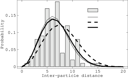
FIG. 1.: Empirical density $p_{\rm emp}$ for $n$ = 100, true likelihood $p_{\rm true}$, reference likelihood $p_{0}$, reconstructed likelihood $p_{\rm IHFA}$ as function of inter–particle distance.

FIG. 2.: True potential $v_{\rm true}$, reference potential $v_{0}$, and reconstructed IHFA potential $v_{\rm IHFA}$ as function of inter–particle distance.

REFERENCES

- [1] R. Newton, Inverse Schrödinger Scattering in Three Dimensions (Springer Verlag, Berlin, 1989).
- [2] K. Chadan, D. Colton, L. Päivärinta, and W. Rundell, An Introduction to Inverse Scattering and Inverse Spectral Problem (SIAM, Philadelphia, 1997).
- [3] A. Tikhonov and V. Arsenin, Solution of Ill–posed Problems (Wiley, New York, 1977).
- [4] A. Kirsch, An Introduction to the Mathematical Theory of Inverse Problems (Springer Verlag, New York, 1996).
- [5] J. Berger, Statistical Decision Theory and Bayesian Analysis (Springer Verlag, New York, 1980).
- [6] C. Robert, The Bayesian Choice (Springer Verlag, New York, 1994).
- [7] A. Gelman, J. Carlin, H. Stern, and D. Rubin, Bayesian Data Analysis (Chapman & Hall, New York, 1995).
- [8] J. Lemm, J. Uhlig, and A. Weiguny, A Bayesian Approach to Inverse Quantum Statistics, cond-mat/9907013.
- [9] R. Neal, Bayesian Learning for Neural Networks (Springer Verlag, New York, 1996).
- [10] C. K. I. Williams and C. E. Rasmussen, in Advances in Neural Information Processing Systems 8, edited by D. S. Touretzky, M. C. Mozer, and M. E. Hasselmo (The MIT Press, Cambridge, MA, 1996), pp. 514–520.
- [11] J. Lemm, in ICANN 99. Proceedings of the 9th International Conference on Artificial Neural Networks, Edinburgh, UK, 7–10 September 1999 (Springer Verlag, London, 1999).
- [12] G. Wahba, Spline Models for Observational Data (SIAM, Philadelphia, 1990).
- [13] F. Girosi, M. Jones, and T. Poggio, Neural Computation 7, 219 (1995).
- [14] J. Eisenberg and W. Greiner, Microscopic Theory of the Nucleus (North–Holland, Amsterdam, 1972).
- [15] P. Ring and P. Schuck, The Nuclear Many–Body Problem (Springer Verlag, New York, 1980).
- [16] J.-P. Blaizot and G. Ripka, Quantum Theory of Finite Systems (The MIT Press, Cambridge, MA, 1986).
- [17] J. C. Lemm, Annals of Physics 244, 136 (1995).