Gravitational coupling to two-particle bound states and momentum conservation in deep inelastic scattering

Abstract

The momentum conservation sum rule for deep inelastic scattering (DIS) from composite particles is investigated using the general theory of relativity. For two $1+1$ dimensional examples, it shown that covariant theories automatically satisy the DIS momentum conservation sum rule provided the bound state is covariantilly normalized. Therefore, in these cases the two DIS sum rules for baryon conservation and momentum conservation are equivalent.

I Introduction

In the parton model of deep inelastic scattering (DIS) from a bound state with $N$ valence quarks, one encounters two sum rules:

$$\sum_{i}n_{i}\int_{0}^{1}f_{i}(x)dx =\sum_{i}n_{i}$$ (1)

$$\sum_{i}\int_{0}^{1}xf_{i}(x)dx =1\,,$$ (2)

where $f_{i}(x)$ is the probability that the quarks of flavor $i$ will have momentum fraction $x$. The first sum rule corresponds to baryon (or charge) conservation and the second to the conservation of the momentum fraction. In a previous work[1], we showed, in the context of a covariant model for the bound state, that the first sum rule is a consequence of the normalization condition for the covariant bound state wave function, and hence is automatically satisfied in any covariant model.

In parton models, the two relations (2) are usually considered to be independent constraints. This could pose a problem for covariant descriptions of DIS because in this formalism the normalization condition is the only constraint which can be imposed on the covariant wave function. It is therefore unclear where the additional momentum conservation constraint could come from. This suggests that either covariant models of DIS are inconsistent, or that the two constraints (2) are somehow not independent and in fact are both a consequence of the normalization condition. This puzzle provided the initial motivation for this work. We will return to discussion of this issue in the concluding section.

In the main part of this paper we turn to another question related to the above issue: “How can we prove, in the context of a covariant treatment of two body bound states, that a static gravitational field couples only to the total mass of the bound state?” In the context of a field theory this requires proving that the coupling of a long wave length graviton to a composite system has the same structure as its coupling to an elementary particle, with the mass replaced by the total mass of the bound state. In this paper we will show, for two simple 1+1 dimensional models, that the bound state normalization condition is sufficient to insure that is indeed the case.

These conservation laws are a consequence of the symmetries of the external field with which the system interacts. For example, the deuteron, which is the bound state of a proton and a neutron, participates in the electromagnetic interaction with a $U(1)$ symmetry. The electromagnetic field couples to each of the constituents separately but if the radiation has a large wavelength, it “sees” only the total charge. Consequently one should be able to compute the total charge of the composite system from the density functions predicted from the bound state model, so one gets a constraint on the bound state. As is well known, this constraint is identical to the bound state normalization condition.

To see how this comes about in the context of the gravitational interaction (related to momentum conservation), we go back to the first principles and consider the interaction of a composite particle in a gravitational field. The requirement that the gravitational field couple to the total bound state mass leads to a constraint which at first seems to be different from the the wave function normalization condition, but we prove that they are compatible.

We start in the next section by reviewing the properties of the gravitational interaction with scalar particles and develop the general framework of our approach. Then we apply our method to the study of some two-particle bound states in $1+1$ dimensions. In Sec. III we study bound states of two scalars, and in Sec. IV bound states of a spin $1/2$ fermion and a scalar. Some conclusions are given in Sec. V.

II Gravitational Interactions with scalar particles

In this section we review the most basic properties of the lowest order graviton-scalar interaction. After we obtain the Feymnan rules of two cubically interacting scalar fields in the environment of a gravitational field, we investigate some Feynman diagrams with a single external graviton line to illustrate momentum conservation in some specific cases. We make use of the gravitational Ward-Takahashi identity, which we first prove by using our previously obtained Feynman rules and prove using a more general field theory argument.

This section is meant to give the general framework of this paper, including the machinery of the bound state-graviton interaction, that will be used in the next sections to derive the constraint imposed on the bound state wave functions by momentum conservation.

A Gravitational Interaction of Scalar Particles

Consider two interacting scalar fields $\Phi$ and $\phi$. We will assume $\Phi$ is charged and that $\phi$ is a neutral, self conjugate field. A gravitational “interaction” is added if the flat metric tensor $\eta^{\mu\nu}=diag[1,-1,-1,-1]$ is replaced by an arbitrary metric $g^{\mu\nu}(x)$,

$$g^{\mu\nu}(x)=\eta^{\mu\nu}+2h^{\mu\nu}(x)\,,$$ (3)

where $h^{\mu\nu}(x)$ is the gravitational field. (Note that our metric differs in sign and that $h^{\mu\nu}$ differs by a factor of 2 from that used by Weinberg[2]). The four-volume element $d^{4}x$ is also replaced by

$$\int d^{4}x\to\int d^{4}x\sqrt{-g}\,,$$ (4)

where $g$ is the determinant of the covariant metric tensor $g_{\mu\nu}$. [Recall that, in curved space, the covariant and contravariant metric tensors are not the same.]

For simplicity, the $\Phi\Phi\phi$ interaction is assumed to be a Yukawa-type, so the Lagrangian reads:

$${\cal L}=g^{\mu\nu}\partial_{\mu}\Phi^{\dagger}\partial_{\nu}\Phi-M^{2}\Phi^{\dagger}\Phi+\frac{1}{2}g^{\mu\nu}\partial_{\mu}\phi\partial_{\nu}\phi-\frac{1}{2}m^{2}\phi^{2}-\lambda\phi\Phi^{\dagger}\Phi,$$ (5)

The kinetic part of the Lagrangian of the scalar fields naturally involves the covariant components of the derivatives of the fields, rather than the contravariant ones. Since the fields are scalars, their plain derivatives are therefore identical to their covariant derivatives, and hence for scalar fields the affine connections

$$\Gamma^{\alpha}_{\mu\nu}=\frac{1}{2}g^{\alpha\beta}(g_{\beta\mu,\nu}+g_{\nu\beta,\mu}-g_{\mu\nu,\beta})$$ (6)

(where $g_{\mu\nu,\beta}=\partial g_{\mu\nu}/\partial x^{\beta}$) usually needed to convert normal derivatives in covariant derivatives, will play no role. This greatly simplifies the discussion of the gravitational interactions of scalar fields. Later, when we discuss spin 1/2 fields in Sec. IV, we will have to deal with the greater complexity introduced by the affine connections.

In four dimensions, the total action for this scalar theory is taken to be[2, 3, 4]

$$S=\int d^{4}x\sqrt{-g}\left[{\cal L}+\frac{1}{2\kappa}R\right]=S_{f}+S_{g}$$ (7)

where

$$\kappa=\frac{8\pi G}{c^{4}}$$

and $R$ is the curvature scalar of the space-time continuum equal to $g^{\mu\nu}R_{\mu\nu}$, where $R_{\mu\nu}$ is the Ricci tensor

$$R_{\mu\nu}=-\Gamma^{\alpha}_{\mu\nu,\alpha}+\Gamma^{\alpha}_{\mu\alpha,\nu}+\Gamma^{\lambda}_{\mu\alpha}\Gamma^{\alpha}_{\lambda\nu}-\Gamma^{\lambda}_{\mu\nu}\Gamma^{\alpha}_{\lambda\alpha}\,.$$ (8)

In the special case of the flat space, $R=0$, and the usual Euler-Lagrange equations result from the application of Hamilton’s principle to the fields $\phi$ and $\Phi$:

$$\eta^{\mu\nu}\partial_{\mu}\partial_{\nu}\phi+m^{2}\phi+\lambda\Phi^{\dagger}\Phi =0$$ (9)

$$\eta^{\mu\nu}\partial_{\mu}\partial_{\nu}\Phi+M^{2}\Phi+\lambda\Phi\phi =0\,.$$ (10)

Quantizing the fields using the path integral formalism gives the Feynman rules:

$$-i{\cal V}_{3}= -i\lambda$$ (11)

$$-i\Delta_{M}(p)= \frac{-i}{M^{2}-p^{2}-i\epsilon}\,,$$ (12)

where ${\cal V}_{3}$ is the Feynman rule of the $\Phi\Phi\phi$ vertex (Fig. 1), and $\Delta_{M}$ is the propagator for the $\Phi$ field. [A similar factor, $\Delta_{m}$, is the propagator for the neutral field $\phi$.] In our Feynman diagrams, the $\Phi$ field is represented by the thick solid line and the $\phi$ field is represented by the thin solid line. We obtain the usual equations of motion and the usual Feynman rules for the limiting case of a flat space.

FIG. 1.: $\Phi\Phi\phi$ interaction.

In four dimnensions the action (7) also yields Einstein’s equations for the field $h^{\mu\nu}$ defined in Eq. (3). Hamilton’s principle for the field $h^{\mu\nu}$ is

$$\frac{\delta}{\delta h^{\mu\nu}}\left[\sqrt{-g}\left({\cal L}+\frac{1}{2\kappa}R\right)\right]=0\,,$$ (13)

and yields the following Euler-Lagrange equations for the gravitational field

$$\frac{1}{\kappa}\left\{R_{\mu\nu}-\frac{1}{2}\,g_{\mu\nu}R\right\}+{\cal T}_{\mu\nu}=0\,.$$ (14)

Here the total energy-momentum tensor ${\cal T}_{\mu\nu}$ is the sum of contributions from the fields $\phi$ and $\Phi$, and an interaction part:

$${\cal T}_{\mu\nu}=T_{\mu\nu}(\phi)+T_{\mu\nu}(\Phi)+T_{\mu\nu}(\phi,\Phi)$$ (15)

$$T_{\mu\nu}(\phi)=\frac{1}{2}(\partial_{\mu}\phi\partial_{\nu}\phi+\partial_{\nu}\phi\partial_{\mu}\phi)-\frac{1}{2}g_{\mu\nu}(g^{\alpha\beta}\partial_{\alpha}\phi\partial_{\beta}\phi-m^{2}\phi^{2})$$ (16)

$$T_{\mu\nu}(\Phi)=\partial_{\mu}\Phi^{\dagger}\partial_{\nu}\Phi+\partial_{\nu}\Phi^{\dagger}\partial_{\mu}\Phi-g_{\mu\nu}(g^{\alpha\beta}\partial_{\alpha}\Phi^{\dagger}\partial_{\beta}\Phi-M^{2}\Phi^{\dagger}\Phi)$$ (17)

$$T_{\mu\nu}(\phi,\Phi)=\lambda g_{\mu\nu}\Phi^{\dagger}\Phi\phi\,.$$ (18)

The ${\cal T}_{\mu\nu}$ term in Eq. (14) can be derived easily once the variation of $\sqrt{-g}$ in terms of $\delta g^{\mu\nu}=2h^{\mu\nu}$ has been calculated. We will carry out this derivation in an arbitrary number of (integral) dimensions $d$. First, exploit the identity

$$g^{\mu\nu}g_{\mu\nu}=d$$ (19)

to obtain the relation

$$g^{\mu\nu}h_{\mu\nu}=-g_{\mu\nu}h^{\mu\nu}\,.$$ (20)

This can also be conveniently rewritten

$$h_{\alpha\beta}=-\frac{1}{d}\,g_{\alpha\beta}\,g_{\mu\nu}h^{\mu\nu}\,.$$ (21)

From this last relation, and the definition of $g$ in $d$ dimensions

$$g=N\epsilon_{d}^{\alpha\beta\cdots}\epsilon_{d}^{\alpha^{\prime}\beta^{\prime}\cdots}\,g_{\alpha\alpha^{\prime}}g_{\beta\beta^{\prime}}\cdots\,,$$ (22)

where $\epsilon_{d}$ is the antisymmetric symbol in $d$ dimensions and $N$ is a sutiable normalization constant, it follows that

$$\delta g =2Nd\,\epsilon^{\alpha\beta\cdots}\epsilon^{\alpha^{\prime}\beta^{\prime}\cdots}\,h_{\alpha\alpha^{\prime}}g_{\beta\beta^{\prime}}\cdots$$ (24)

$$=-2g\,g_{\mu\nu}h^{\mu\nu}\,,$$

and therefore

$$\delta\sqrt{-g}=-\sqrt{-g}\,g_{\mu\nu}h^{\mu\nu}.$$ (25)

On the other hand

$$\frac{\delta{\cal L}}{\delta h^{\mu\nu}}=2\partial_{\mu}\Phi^{\dagger}\partial_{\nu}\Phi+\partial_{\mu}\phi\partial_{\nu}\phi.$$ (26)

Putting Eqs. (25) and (26) together, and symmetrizing (26), we see that:

$$\delta\int d^{4}x\sqrt{-g}\,{\cal L}=\int d^{4}x\sqrt{-g}\,{\cal T}_{\mu\nu}\,h^{\mu\nu}\,.$$ (27)

The first two terms in Eq. (14) arise from the variation of $S_{g}$ in four dimensions[2, 4]

$$\delta\left(\frac{1}{2\kappa}\int d^{4}x\sqrt{-g}R\right)=\frac{1}{\kappa}\int d^{4}x\sqrt{-g}\,(R_{\mu\nu}-\frac{1}{2}g_{\mu\nu}R)\,h^{\mu\nu}\,.$$ (28)

Setting the combined variations (27) and (28) to zero gives the field equations (14). These are Einstein’s equations for the gravitational “interaction”[2] and hence the action (7) gives the correct classical relation for the gravitational field in addition to the right flat space limit.

It will turn out that Eq. (28) must be modified for the applications to 1+1 dimensional space studied in this paper (see the discussion in Subsection B below). This leads to a modification of the field equation (14) in 1+1 dimensions. However, the derivation of the coupling of the gravitational field to matter, given in Eq. (27), is, as we have seen, independent of dimension, and we can derive the Feynman rules which describe the coupling of a graviton to matter directly from it. We will only consider the gravitational interaction to lowest order (weak field limit) and will represent the gravitational interaction by a dashed line. The Feynman rules, besides the ones given in Eqs. (12), contain two matter field-graviton vertices (Fig 2).

FIG. 2.: $\Phi\Phi$-graviton and $\phi\phi$-graviton interaction.

The Feynman rule of these vertices is:

$$-i{\cal J}_{M}^{\mu\nu}(p^{\prime},p)=i\left[p^{\mu}p^{\prime\nu}+p^{\nu}p^{\prime\mu}+\eta^{\mu\nu}(M^{2}-p\cdot p^{\prime})\right]\,.$$ (29)

The $\phi\phi$-graviton vertex has the same form, as expected from the fact that charged and uncharged particles interact in the same way with a gravitational field.

This Feynman rule can be derived from the flat space limit of Eq. (27)

$$\delta\left(i\int d^{4}x\sqrt{-g}{\cal L}\right)\simeq i\int d^{4}x{\cal T}_{\mu\nu}(x)h^{\mu\nu}(x)\,.$$ (30)

Sandwiching this result between the incoming and outgoing $\Phi$ (or $\phi$) states gives

$$\delta\left(i<p^{\prime}|\int d^{4}x\sqrt{-g}{\cal L}|p>\right)\simeq i\int d^{4}x<p^{\prime}|{\cal T}_{\mu\nu}(x)|p>h^{\mu\nu}(x)\,.$$ (31)

Reducing this expression gives

$$\delta\left(i<p^{\prime}|\int d^{4}x\sqrt{-g}{\cal L}|p>\right)$$ (32)

$$\qquad\qquad\simeq i\left[p_{\mu}p^{\prime}_{\nu}+p_{\nu}p^{\prime}_{\nu}+\eta_{\mu\nu}(M^{2}-p\cdot p^{\prime})\right]\int d^{4}xh^{\mu\nu}(x)e^{i(p^{\prime}-p)\cdot x}$$ (33)

$$\qquad\qquad=i\left[p_{\mu}p^{\prime}_{\nu}+p_{\nu}p^{\prime}_{\nu}+\eta_{\mu\nu}(M^{2}-p\cdot p^{\prime})\right]{\tilde{h}}^{\mu\nu}(p^{\prime}-p)\,,$$ (34)

where ${\tilde{h}}^{\mu\nu}(p^{\prime}-p)$ is the Fourier transform of the gravitational field. Hence the coupling given in Eq. (29) [which is the coefficient of the ${\tilde{h}}^{\mu\nu}$ term in $\delta{\cal L}$] emerges. Although this derivation assumes that the gravitational field is not quantized, Eq. (29) is correct even in the case of quantized gravitational fields, as one will see in Subsection C.

The model likewise involves a $\Phi\Phi\phi$-graviton coupling (Fig.3),

FIG. 3.: $\Phi\Phi\phi$- graviton vertex

its Feynman rule being:

$$-i{\cal V}_{\mu\nu}^{3}=i\lambda\eta_{\mu\nu}.$$ (35)

The vertex ${\cal V}_{\mu\nu}$ has a physical interpretation: it is the ”weight” of the vertex ${\cal V}$. In the non-quantized theory of the point-like particles, the gravity couples to the energy-momentum tensor, which may have a part coming from an interaction. Our interpretation is consistent with the limiting case. Note the obvious, model independent generalization:

$$-i{\cal V}_{\mu\nu}^{3}=i\eta_{\mu\nu}{\cal V}^{3},$$ (36)

All these vertices involving gravitons are symmetric in the Lorentz indices, and so is the external gravitational field $h^{\mu\nu}$.

In addition to these interactions, the theory involves a graviton propagator, graviton-graviton interactions and several-graviton -matter field vertices, which we do not display. Because we are interested in first order gravitational interactions between a bound state of two $\Phi$ particles and an external (non-quantized) weak gravitational field, we can safely ignore these undisplayed rules.

In the next subsection we extend our discussion of the field equations to 1+1 dimensional space and describe the constraints on the gravitational couplings which emerge from gauge invariance.

B Gravitational Coupling and Gauge Invariance

Because the gravitational action does not contain a mass term, scattering amplitudes at any order are expected to be gauge invariant. [The cosmological term[4] would destroy this symmetry, but if it is non-zero it is at least very small, so gauge invariance is either exact or a very good approximation.] In four dimensions this follows from Eq. (14); the covariant divergence of the $1/\kappa$ term vanishes identically, insuring that the energy momentum tensor is conserved. In addition, the gravitational trace of Eq. (14) yields the result

$$\left(\frac{d}{2}-1\right)\,R=\kappa\,g^{\mu\nu}{\cal T}_{\mu\nu}\,.$$ (37)

Note that this equation cannot be correct in $d=2$ dimensions, where the LHS would be zero and the RHS non-zero. This is one indication that the Eq. (14) is not correct in two (i.e. 1+1) dimensions.

For our purposes it is sufficient to find the correct equation in the weak gravitational field limit. Eq. (14) reduces to [4]

$$\partial^{2}h^{\mu\nu}-\partial_{\lambda}\partial^{\nu}h^{\mu\lambda}-\partial_{\lambda}\partial^{\mu}h^{\nu\lambda}+\eta^{\mu\nu}\partial_{\lambda}\partial_{\sigma}h^{\lambda\sigma}+\partial^{\mu}\partial^{\nu}h-\eta^{\mu\nu}\partial^{2}h=-\kappa{\cal T}^{\mu\nu}\,,$$ (38)

where $\partial^{2}=\partial_{\lambda}\partial^{\lambda}$ and $h=\eta_{\alpha\beta}h^{\alpha\beta}$. As expected, the trace of the LHS is zero in 2 dimensions (to lowest order it is sufficient to calculate this trace by contracting with $\eta_{\mu\nu}$). However, as discussed by Ohanian and Ruffini[4], the following replacement

$$h^{\mu\nu}=\bar{h}^{\mu\nu}-\frac{1}{2}(1-a)\;\eta^{\mu\nu}\bar{h}\,,$$ (39)

transforms Eq. (38) to

$$\partial^{2}\bar{h}^{\mu\nu}-\partial_{\lambda}\partial^{\nu}\bar{h}^{\mu\lambda}-\partial_{\lambda}\partial^{\mu}\bar{h}^{\nu\lambda}+\eta^{\mu\nu}\partial_{\lambda}\partial_{\sigma}\bar{h}^{\lambda\sigma}+a\left(\partial^{\mu}\partial^{\nu}\bar{h}-\eta^{\mu\nu}\partial^{2}\bar{h}\right)=-\kappa{\cal T}^{\mu\nu}\,,$$ (40)

showing that the coefficient $a$ is arbitrary (except it cannot be 1/2 because this choice would force $\eta_{\mu\nu}h^{\mu\nu}=0$). Since $h^{\mu\nu}$ is symmetric, the divergence of the LHS of Eq. (40) with respect to either index is zero, and the stress energy tensor is conserved for any value of $a$

$$\partial_{\mu}{\cal T}^{\mu\nu}=0=\partial_{\mu}{\cal T}^{\nu\mu}\,.$$ (41)

This is analogous to the conservation of electromagnetic current. However, the trace condition obtained from Eq. (40) now depends on $a$ and is not zero unless $d=2$ and $a=1$

$$(1+a-ad)\partial^{2}\bar{h}+(d-2)\partial_{\mu}\partial_{\nu}\bar{h}^{\mu\nu}=-\kappa\,\eta_{\mu\nu}{\cal T}^{\mu\nu}=(1-a)\partial^{2}\bar{h}\,,$$ (42)

where the last form of the equation holds in $d=2$ dimensions. We will not persue the formal development of the 2 dimensional theory further. We will imagine that the gravitational field in 2 dimensions is given by Eqs. (40) and (42) with $a\neq 1$.

Because of the symmetry under interchange of indices, the gravitational gauge invariance is described by a $U(1)\times U(1)$ group and we may check the gauge invariance for the case of one index only. In momentum space the requirements (41) therefore become, in the linear approximation,

$$q_{\mu}{\cal T}^{\mu\nu}=0\,,$$ (43)

where $q$ is the momentum of the graviton. Let us proceed by verifying gravitational gauge invariance for some simple cases.

First consider the graviton-$\Phi\Phi$ vertex given in Eq. (29) and shown in Fig. 2. If neither of the $\Phi$ mesons is on-shell, the divergence of the interaction term (29) gives the following Ward-Takahashi identity:

$$q_{\mu}{\cal J}^{\mu\nu}_{M}(p^{\prime},p)=p^{\nu}\Delta_{M}^{-1}(p^{\prime})-p^{\prime\nu}\Delta_{M}^{-1}(p)\,,$$ (44)

where $p^{\prime}$ and $p$ are the final and initial momentum of the particles and $q=p^{\prime}-p$. If the particles are on-shell, the inverse propagators vanish, so the vertex is gauge invariant. The graviton-$\phi\phi$ vertex is similarly gauge invariant for on-shell $\phi$ particles, and its Ward-Takahashi identity is the same, with $M$ replaced by $m$. A more complete description of the graviton-scalar interaction can be found in [6].

The gravitational Ward-Takahashi identities are important relations needed to verify the gauge invariance of the higher order diagrams. Therefore, before going further in checking some other diagrams, we will devote the next subsection to a model- independent proof of this important identity.

C Ward-Takahashi Identities

In this subsection we derive the gravitational Ward-Takahashi identity for any scalar field in a model independent way. A derivation has been given by West [7], but here we follow a different path based on ideas borrow from references [8] and [9], where the Ward-Takahashi identity has been derived for QED and QCD.

We start with the field theoretic matrix element:

$$(2\pi)^{d} \delta^{(d)}(p+q-p^{\prime})\Delta_{M}(p^{\prime}){\cal J}_{\mu\nu}(p^{\prime},p)\Delta_{M}(p)$$ (46)

$$=\frac{1}{2}\int d^{d}xe^{-ip^{\prime}\cdot x}\int d^{d}ye^{iq\cdot y}\int d^{d}ze^{ip\cdot z}<0|T\left(\Phi(x){T}_{\mu\nu}(y)\Phi^{\dagger}(z)\right)|0>\,,$$

where $T_{\mu\nu}(y)=T_{\mu\nu}(\Phi(y))$ was given in Eq. (18), and the factor of one-half on the RHS insures that the ${\cal J}_{\mu\nu}$ given on the LHS agrees with our definition (29). Translating the fields (where ${\hat{p}}$ is the momentum operator)

$$\Phi^{\dagger}(z)= e^{-i{\hat{p}}\cdot\eta}\Phi^{\dagger}(z-\eta)e^{i{\hat{p}}\cdot\eta}$$ (47)

$${T}_{\mu\nu}(y)= e^{-i{\hat{p}}\cdot\eta}{T}_{\mu\nu}(y-\eta)e^{i{\hat{p}}\cdot\eta}$$ (48)

$$\Phi(x)= e^{-i{\hat{p}}\cdot\eta}\Phi(x-\eta)e^{i{\hat{p}}\cdot\eta}$$ (49)

changes the time ordered product to:

$$T\left(\Phi(x){T}_{\mu\nu}(y)\Phi^{\dagger}(z)\right)=T\left(e^{-i{\hat{p}}\cdot\eta}\Phi(x-\eta){T}_{\mu\nu}(y-\eta)\Phi^{\dagger}(z-\eta)e^{i{\hat{p}}\cdot\eta}\right)\,.$$ (50)

Letting $\eta=(x+z)/2$, changing variables

$$x-\eta =\frac{1}{2}(x-z)\rightarrow\frac{1}{2}\zeta$$ (51)

$$y-\eta \rightarrow y\,,$$ (52)

and integrating over $\eta$, transforms (46) into

$$\Delta_{M}(p^{\prime}) {\cal J}_{\mu\nu}(p^{\prime},p)\Delta_{M}(p)$$ (53)

$$= \frac{1}{2}\int d^{d}\zeta e^{-i(p^{\prime}+p)\cdot\frac{1}{2}\zeta}\int d^{d}ye^{iq\cdot y}<0|T\left(\Phi\left({\textstyle\frac{1}{2}}\zeta\right){T}_{\mu\nu}(y)\Phi^{\dagger}\left(-{\textstyle\frac{1}{2}}\zeta\right)\right)|0>\,,$$ (54)

where we have used the translational invariance of the vacuum. Dotting this equation with $q$, and integrating by parts, gives

$$q^{\mu}\Delta_{M}(p^{\prime}) {\cal J}_{\mu\nu}(p^{\prime},p)\Delta_{M}(p)$$ (55)

$$= \frac{i}{2}\int d^{d}\zeta e^{-i(p^{\prime}+p)\cdot\frac{1}{2}\zeta}\int d^{d}ye^{iq\cdot y}\frac{\partial}{\partial y_{\mu}}<0|T\left(\Phi\left({\textstyle\frac{1}{2}}\zeta\right){T}_{\mu\nu}(y)\Phi^{\dagger}\left(-{\textstyle\frac{1}{2}}\zeta\right)\right)|0>\,.$$ (56)

Since ${T}_{\mu\nu}$ is divergenceless, the divergence of the temporal product in (56) reduces to

$$\frac{\partial}{\partial y_{\mu}}T\left(\Phi{T}_{\mu\nu}\Phi^{\dagger}\right)$$ (57)

$$=\delta(y_{0}-{\textstyle\frac{1}{2}}\zeta_{0})\left(\theta(\zeta_{0})\left[{T}_{0\nu}(y),\Phi\left({\textstyle\frac{1}{2}}\zeta\right)\right]\Phi^{\dagger}\left(-{\textstyle\frac{1}{2}}\zeta\right)+\theta(-\zeta_{0})\Phi^{\dagger}\left(-{\textstyle\frac{1}{2}}\zeta\right)\left[{T}_{0\nu}(y),\Phi\left({\textstyle\frac{1}{2}}\zeta\right)\right]\right)$$ (58)

$$+\delta(y_{0}+{\textstyle\frac{1}{2}}\zeta_{0})\left(\theta(\zeta_{0})\Phi\left({\textstyle\frac{1}{2}}\zeta\right)\left[{T}_{0\nu}(y),\Phi^{\dagger}\left(-{\textstyle\frac{1}{2}}\zeta\right)\right]+\theta(-\zeta_{0})\left[{T}_{0\nu}(y),\Phi^{\dagger}\left(-{\textstyle\frac{1}{2}}\zeta\right)\right]\Phi\left({\textstyle\frac{1}{2}}\zeta\right)\right).$$ (59)

Using the relation

$$\delta(y_{0}-{\textstyle\frac{1}{2}}\zeta_{0})\left[{T}_{0\nu}(y),\Phi\left({\textstyle\frac{1}{2}}\zeta\right)\right]=-i\delta^{(d)}({y}-{\textstyle\frac{1}{2}}\zeta)\frac{\partial\Phi(y)}{\partial y^{\nu}}$$ (60)

and substituting it into the Eq. (59) gives

$$\frac{\partial}{\partial y_{\mu}} T\left(\Phi{T}_{\mu\nu}\Phi^{\dagger}\right)$$ (61)

$$= -i\delta^{(d)}(y-{\textstyle\frac{1}{2}}\zeta)\left(\theta(\zeta_{0})\frac{\partial\Phi(y)}{\partial y^{\nu}}\Phi^{\dagger}\left(-{\textstyle\frac{1}{2}}\zeta\right)+\theta(-\zeta_{0})\Phi^{\dagger}\left(-{\textstyle\frac{1}{2}}\zeta\right)\frac{\partial\Phi(y)}{\partial y^{\nu}}\right)$$ (63)

$$-i\delta^{(d)}(y+{\textstyle\frac{1}{2}}\zeta)\left(\theta(\zeta_{0})\Phi\left({\textstyle\frac{1}{2}}\zeta\right)\frac{\partial\Phi^{\dagger}(y)}{\partial y^{\nu}}+\theta(-\zeta_{0})\frac{\partial\Phi^{\dagger}(y)}{\partial y^{\nu}}\Phi\left({\textstyle\frac{1}{2}}\zeta\right)\right)$$

$$= -i\delta^{(d)}(y-{\textstyle\frac{1}{2}}\zeta)\frac{\partial}{\partial y^{\nu}}\,T\left(\Phi(y)\Phi^{\dagger}\left(-{\textstyle\frac{1}{2}}\zeta\right)\right)-i\delta^{(d)}(y+{\textstyle\frac{1}{2}}\zeta)\frac{\partial}{\partial y^{\nu}}\,T\left(\Phi\left({\textstyle\frac{1}{2}}\zeta\right)\Phi^{\dagger}(y)\right)\,.$$ (64)

Substituting this expression into (56), integrating over $y$, and then integrating by parts over $\zeta$ gives

$$q^{\mu}\Delta_{M}(p^{\prime}){\cal J}_{\mu\nu}(p^{\prime},p)\Delta_{M}(p)= i\int d^{d}\zeta e^{-ip\cdot\zeta}\;p^{\nu}<0|T\left(\Phi\left({\textstyle\frac{1}{2}}\zeta\right)\Phi^{\dagger}\left(-{\textstyle\frac{1}{2}}\zeta\right)\right)|0>$$ (66)

$$-i\int d^{d}\zeta e^{-ip^{\prime}\cdot\zeta}\;p^{\prime\nu}<0|T\left(\Phi\left({\textstyle\frac{1}{2}}\zeta\right)\Phi^{\dagger}\left(-{\textstyle\frac{1}{2}}\zeta\right)\right)|0>\,.$$

Finally, using the definition of the propagator [with the sign convention of Eq. (12)]

$$i\int d^{d}\zeta e^{ip^{\prime}\cdot\zeta}<0|T\left(\Phi\left({\textstyle\frac{1}{2}}\zeta\right)\Phi^{\dagger}\left(-{\textstyle\frac{1}{2}}\zeta\right)\right)|0>=\Delta_{M}(p^{\prime})\,,$$ (67)

Eq. (66) becomes:

$$q^{\mu}\Delta_{M}(p^{\prime}){\cal J}_{\mu\nu}(p^{\prime},p)\Delta_{M}(p)=p_{\nu}\Delta_{M}(p)-p^{\prime}_{\nu}\Delta_{M}(p^{\prime}).$$ (68)

Canceling $\Delta(p^{\prime})$ and $\Delta_{M}(p)$ from the LHS of Eq. (68), we get the gravitational Ward-Takahashi identity for any bosonic field:

$$q^{\mu}{\cal J}_{\mu\nu}(p^{\prime},p)=p_{\nu}\Delta_{M}^{-1}(p^{\prime})-p^{\prime}_{\nu}\Delta_{M}^{-1}(p)\,.$$ (69)

Our proof of the Eq. (69) is dimension independent.

FIG. 4.: The $\Phi+\phi\to\Phi+h$ interaction to lowest order in $\lambda$.

FIG. 5.: The radiative OBE diagrams to second order in $\lambda$.

Similarly we can repeat this proof for any fermionic field, but we would have some sign differences in Eq. (59) and we would need to use anticommutation relations to redcuce the commutators to delta function. Hence the proof becomes model independent. Next we will investigate the gauge invariance of some other diagrams.

D Gauge Invariance of Some Three-, Four- and Five-Point Functions

Using the Ward-Takahashi identities we have derived, it is easy to show that the contributions from the four diagrams shown in Fig. 4 describing the scattering of $\Phi+\phi\to\Phi+h$ (where $h$ is the gravitation) are gauge invariant.

Similarily, the seven OBE (one boson exchange) diagrams shown in Fig. 5, that describe graviton emmession from the lowest order $\phi$ exchange contribution to $\Phi\Phi$ scattering are also gauge invariant.

To investigate the gauge invariance of the gravitational coupling to the bound state of two $\Phi$-particles, we must first define the Bethe-Salpeter vertex for the $\Phi\Phi$ bound state. In the ladder approximation, the bound state propagator is generated from the infinite ladder sum (illustrated in Fig. 6), and the bound state vertex is a solution of the ladder Bethe-Salpeter equation, illustrated in Fig.7. With this description, the gravitional coupling to the $\Phi\Phi$ bound state is described exactly by the three diagrams shown in Fig. 8, and is gauge invariant. The diagram 8(a) containing no internal $\phi$ lines and the diagram 8(c) which involves a four-particle vertex contribute twice (once for each $\Phi$ particle) and their sum is gauge invariant by itself. The diagram 8(b) contributes only once and is also separately gauge invariant. The proof follows from the Ward-Takahashi identies and does not depend on the explicit form of the propagators or bound state vertices. In a similar fashion any $\phi^{3}$ theory, such as QED, is gauge invariant[5].

FIG. 6.: The $\phi$ ladder diagrams used to construct a $\Phi\Phi$ bound state.

FIG. 7.: The ladder Bethe-Salpeter equation for the $\Phi\Phi$ bound state.

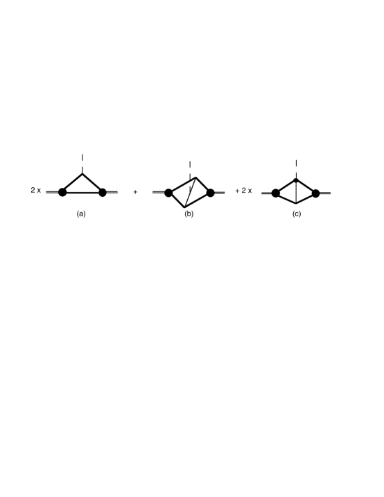
FIG. 8.: The gravitional coupling to the $\Phi\Phi$ bound state in Bethe-Salpeter ladder approximation.

How can we demonstrate the gauge invariance of a generic $\varphi^{4}$-type theory? No separate proof is necessary since the $\varphi^{3}$-type theories are gauge invariant and from any $\Phi^{\dagger}\Phi\phi$ model a generic $\varphi^{4}$-type theory can be obtained directly by making the $\phi$ fields heavy and shrinking the internal $\phi$ propagators to a point (in this example the theory will have a point-like $(\Phi^{\dagger}\Phi)^{2}$ structure). In this way we obtain a effective field theory without loss of gauge invariance. After this reasoning we can assume that all $\varphi^{4}$-type theories are gravitionally gauge invariant.

These examples illustrate gravitational gauge invariance explicitly. All of the diagrams of a given order, and certain infinite classes of diagrams, are gravitionally gauge invariant. A consequence of this is that the gravitational field must couple to the total energy-momentum tensor of a composite system, and this coupling, which depends on the bound state mass, must be consistent with other ways of computing the bound state mass. In the following sections we will study the implications of this consistency requirement for an effective $\varphi^{4}$-type field theory of gravitation.

E Gravitational Coupling in an Effective Field Theory

In this subsection we work out details of the gravitational coupling for an effective field theory (EFT) with a $(\Phi^{\dagger}\Phi)^{2}$ structure. As discussed above, this EFT is obtained from the $\Phi^{\dagger}\Phi\phi$ theory by letting the mass $m$ of the $\phi$ particle go to infinity, and shrinking all $\phi$ propagators to a point. This EFT would be a valid approximation if the $\Phi$ particles have low momenta and the $\phi$ particles are very heavy.

FIG. 9.: The $\Phi$ four-point coupling.

FIG. 10.: The $\Phi$-graviton five-point coupling.

This theory involves three couplings: an effective $(\Phi^{\dagger}\Phi)^{2}$ four point coupling, a $\Phi^{\dagger}\Phi h$ coupling, and a new effective $(\Phi^{\dagger}\Phi)^{2}\,h$ interaction. The first two vertices were discussed previously. The effective $(\Phi^{\dagger}\Phi)^{2}$ coupling, derived from the OBE model discussed above by shrinking the $\phi$ propagator to a point, is

$$-i{\cal V}_{4}=i\frac{\lambda^{2}}{m^{2}}=ig\,,$$ (70)

where $g$ is the effective $\varphi^{4}$ coupling illustrated in Fig. 9. According to the relation (36), this vertex implies the existence of a $(\Phi^{\dagger}\Phi)^{2}\,h$ five-point coupling of the form:

$$-i{\cal V}^{e}_{\mu\nu}=i\eta_{\mu\nu}{\cal V}_{4}=-i\eta_{\mu\nu}\frac{\lambda^{2}}{m^{2}}=-i\eta_{\mu\nu}g\,.$$ (71)

which is shown in Fig. 10. On the other hand, consistency requires that this five-point vertex also be obtained by shrinking the three diagrams shown in Fig. 11.

FIG. 11.: The three OBE $\Phi$-graviton diagrams which give the effective $\Phi$-graviton five-point coupling illustrated in Fig. 10.

To prove this consistency, we compute each of the diagrams in Fig. 11. Diagram 11(a), in the limit of low external momenta and low momentum transfer, becomes:

$$-i{\cal M}_{a}= \lambda^{2}\Delta_{m}(k)(-i{\cal J}^{m}_{\mu\nu})\Delta_{m}(k-q)$$ (72)

$$\simeq \frac{\lambda^{2}}{m^{2}}(i\eta_{\mu\nu}m^{2})\frac{1}{m^{2}}$$ (73)

$$\simeq i\eta_{\mu\nu}\frac{\lambda^{2}}{m^{2}}\,,$$ (74)

where $k=p_{1}-p_{1}^{\prime}$ and $q$ is the momentum of the outgoing graviton. Note that, at small momenta, Eq. (29) gives $-{\cal J}^{m}_{\mu\nu}\simeq\eta_{\mu\nu}m^{2}$. The contribution from the second diagram, 11(b), is:

$$-i{\cal M}_{b}= -i\Delta_{m}(k-q)(i\lambda\eta_{\mu\nu})(-i\lambda)$$ (75)

$$\simeq -i\eta_{\mu\nu}\frac{\lambda^{2}}{m^{2}}\,.$$ (76)

The contribution from diagram 11(c) in the low momemtum limit is equal to 11(b), and hence the total contribution from diagrams (a)–(c) is

$$-i({\cal M}_{a}+{\cal M}_{b}+{\cal M}_{c})\simeq-i\eta_{\mu\nu}\frac{\lambda^{2}}{m^{2}}=-i\eta_{\mu\nu}g\,,$$ (77)

in full agreement with the Eq. (71). We have shown that the five-point vertex of EFT emerges from the low momentum limit of the “full” theory. We will now use this understanding to obtain an effective description of the bound state.

In the following discussion, we will skip back and forth between the “exact” theory (which includes the OBE description of the interaction) and the EFT (in which the interaction is contracted to a point). We emphasize that these theories are equivalent at small momentum.

At low momenta, the dressed $\Phi\Phi$ scattering amplitude can be calculated in two ways that are equivalent at low momenta: by adding the ladder diagrams of Fig. 6, or by summing the bubbles resulting from the effective four-point interaction illustrated in Fig. 9. In either case, the infinite sum generates the bound state. The gravitational interaction with the bound state can also be described in two different ways, which are equivalent at low momenta. The first of these, illustrated in Fig. 8, is the description in the “exact” theory. The second, shown in Fig. 12, is the description in the EFT.

FIG. 12.: Graviton coupling to the bound state in the $(\Phi^{\dagger}\Phi)^{2}$ EFT.

In either theory, the momentum conservation implied by the gauge invariance of the gravitational interaction implies that the effective graviton-bound state interaction at low momentum transfer must be proportional to the energy momentum tensor of the bound state

$$-i{\cal J}_{M_{b}}^{\mu\nu}(p^{\prime},p)=i\left[p^{\mu}p^{\prime\nu}+p^{\nu}p^{\prime\mu}+g^{\mu\nu}(M_{b}^{2}-p\cdot p^{\prime})\right]\,.$$ (78)

The interactions shown in Figs. 8 and 12 must reproduce this result as the momentum of the graviton $q\to 0$. This requirement places a constraint in the bound state wave function. As we have shown, it is sufficient to study this constraint in the context of the EFT, and this is the subject of the following sections.

III The Mass of a Composite System of Scalars

Using the EFT discussed in the previous section, the tensor (78) must be the sum of the two contributions shown in Fig. 12

$$-i{\cal J}_{M_{b}}^{\mu\nu}(P+q,P)=-2i{\cal J}_{a}^{\mu\nu}(P+q,P)-i{\cal J}_{b}^{\mu\nu}(P+q,P)\,,$$ (79)

where ${\cal J}_{a}^{\mu\nu}$ and ${\cal J}_{b}^{\mu\nu}$ are the contributions from diagrams 12(a) and 12(b), respectively. The factor of 2 multiplying ${\cal J}_{a}$ displays the fact that it occurs twice, once for each constituent. These diagrams are

$$-i{\cal J}_{a}^{\mu\nu}(P+q,P)=-{\cal N}^{2}\int\frac{d^{d}k}{(2\pi)^{d}}\Delta_{M}(P-k)\Delta_{M}(k+q){\cal J}^{\mu\nu}_{M}(k+q,k)\Delta_{M}(k)\,,$$ (80)

where ${\cal N}$ as the bound state vertex function (constant in the EFT), and

$$-i{\cal J}_{b}^{\mu\nu}(P+q,P)=ig\eta^{\mu\nu}{\cal N}^{2}b\left((P+q)^{2}\right)b(P^{2})\,,$$ (81)

where, in 1+1 dimension, the bubble $b$ is

$$b(P^{2})=i\int\frac{d^{d}k}{(2\pi)^{d}}\frac{1}{(M^{2}-k^{2})[M^{2}-(P-k)^{2}]}\,,$$ (82)

as given in Ref. [1].

In Ref. [1] we showed that the vertex function (or normalization constant) ${\cal N}$ and the coupling constant $g$ are related to the bound state mass by

$${\cal N}=\left(-\frac{\partial b(M_{b}^{2})}{\partial M_{b}^{2}}\right)^{-1/2}\qquad\qquad g=\frac{1}{b(M_{b}^{2})}\,,$$ (83)

Requiring the initial and final bound states to be on shell, so the $P^{2}=M_{b}^{2}$ and $(P+q)^{2}=M_{b}^{2}$, permits us to rewrite Eq. (81):

$$-i{\cal J}_{b}^{\mu\nu}=i\eta^{\mu\nu}{\cal N}^{2}b(M_{b}^{2})\,.$$ (84)

Before we use Eq. (79) to calculate the bound state mass, we will prove that this expression is gauge invariant. First, compute $-iq_{\mu}{\cal J}_{a}^{\mu\nu}$

$$-iq_{\mu}{\cal J}_{a}^{\mu\nu} (P+q,P)$$ (85)

$$= -{\cal N}^{2}\int\frac{d^{d}k}{(2\pi)^{d}}\Delta_{M}(P-k)\Delta_{M}(k+q)q_{\mu}{\cal J}^{\mu\nu}_{M}(k+q,k)\Delta_{M}(k)$$ (86)

$$= -{\cal N}^{2}\int\frac{d^{d}k}{(2\pi)^{d}}k^{\nu}\Delta_{M}(P-k)\Delta_{M}(k)+{\cal N}^{2}\int\frac{d^{d}k}{(2\pi)^{d}}(k+q)^{\nu}\Delta_{M}(P-k)\Delta_{M}(k+q)$$ (87)

$$= -iq^{\nu}{\cal N}^{2}\frac{1}{2}\,b(M_{b}^{2})\,.$$ (88)

The transition from the second line was done by using the Ward-Takahashi identity. In the last step we symmetrized the integrands ($k\to k+P/2$ in the ifrst integral and $k\to k+(P-q)/2$ in the second), droped the odd $k^{\nu}$ term, and extracted the final result using the definition (82). Recall that this term must be multiplied by 2, and is cancelled exactly by the term from Eq. (84), which is

$$-iq_{\mu}{\cal J}_{b}^{\mu\nu}=iq^{\nu}{\cal N}^{2}b(M_{b}^{2})\,.$$ (89)

Hence, the sum of the diagrams from Fig. 12 is gauge invariant.

We now use Eq. (79) to “calculate” the square of the bound state mass in 1+1 dimension. Setting $q=0$ and contracting the indices in the Eq. (78) projects out the bound state mass:

$$\eta_{\mu\nu}{\cal J}_{M_{b}}^{\mu\nu}(P,P)=-2M_{b}^{2}\,.$$ (90)

Our goal is to demonstrate that Eq. (79) is indeed consistent with the above result.

First notice that, for off-shell particles in 1+1 $d$,

$$\eta_{\mu\nu}{\cal J}_{M}^{\mu\nu}(k,k)\Delta_{M}^{2}(k)= 2M^{2}\frac{\partial\Delta_{M}(k)}{\partial M^{2}}\,$$ (91)

and hence the contraction of Eq. (79) gives

$$-i\eta_{\mu\nu}{\cal J}_{M_{b}}^{\mu\nu}(P,P)= 2iM_{b}^{2}$$ (92)

$$= -2{\cal N}^{2}\int\frac{d^{d}k}{(2\pi)^{d}}\Delta_{M}(P-k)2M^{2}\frac{\partial\Delta_{M}(k)}{\partial M^{2}}+2i{\cal N}^{2}b(M_{b}^{2})$$ (93)

$$= 2i{\cal N}^{2}\left(M^{2}\frac{\partial}{\partial M^{2}}+1\right)b(M_{b}^{2})\,.$$ (94)

Replacing ${\cal N}^{2}$ by the normalization condition (83) allows us to transform this result into the following condition

$$\left[M^{2}_{b}\frac{\partial}{\partial M_{b}^{2}}+M^{2}\frac{\partial}{\partial M^{2}}+1\right]b(M_{b}^{2})=0\,.$$ (95)

To verify the validity of Eq. (95), we recall that the explicit form of $b$ (taken from Ref. [1], with $m_{1}=m_{2}=M$) is

$$b(M_{b}^{2})=-\frac{1}{4\pi}\int\frac{dx}{M^{2}-M^{2}_{b}x(1-x)}\,.$$ (96)

This satisfies the condition (95). Consequently, we have shown that the normalization condition, Eq. (81), also insures that the graviton couples to the total mass of the bound state, as required by energy- momentum conservation. Since the normalization condition originally came from baryon number conservation (as discussed in Ref. [1]), we conclude that energy-momentum conservation and baryon number conservation are different aspects of the same constraint.

IV Bound State of a Spin $1/2$ Fermion and a Scalar Boson

In this section we extend the preceding results to the case of a bound state of a scalar and a spin $1/2$ fermion, still in $1+1$ dimensions. As above, we assume an effective four-point contact interaction of the form $\lambda(\Psi^{\dagger}\Psi)(\Phi^{\dagger}\Phi)$, as described in Ref. [1]. We start by reviewing the results of the bound state calculations from Ref. [1], and then describe the graviton-spinor interaction. We conclude the section with a detailed treatment of the bound state.

A Bound State Formalism and Normalization

The scattering amplitude (droping the initial and final spinors) for this $\varphi^{4}$-type interaction depends only on the total momentum, $p$, and can be written

$${\cal M}= \frac{\lambda}{1-\lambda\left(A(p^{2})+\not{p}B(p^{2})\right)}$$ (97)

$$= \frac{\lambda(1-\lambda A(p^{2})+\lambda B(p^{2})\not{p})}{(1-\lambda A(p^{2}))^{2}-\lambda^{2}B^{2}(p^{2})p^{2}}\,,$$ (98)

where the spin 1/2 bubble is $A(p^{2})+B(p^{2})\not{p}$, and the functions $A(p^{2})$ and $B(p^{2})$ are

$$A(p^{2})=-\frac{m_{1}}{4\pi}\int^{1}_{0}\frac{dx}{m^{2}_{1}x+m^{2}_{2}(1-x)-p^{2}x(1-x)}$$ (99)

$$B(p^{2})=-\frac{1}{4\pi}\int^{1}_{0}\frac{(1-x)dx}{m^{2}_{1}x+m^{2}_{2}(1-x)-p^{2}x(1-x)}\,,$$ (100)

with $m_{1}$ the mass of the fermion and $m_{2}$ the mass of the boson. If the bound state mass is $M_{b}$, the scattering amplitude ${\cal M}$ should have a pole at $p^{2}=M_{b}^{2}$, which implies

$$1-\lambda A(M_{b}^{2})=\lambda M_{b}B(M_{b}^{2})\,.$$ (101)

Using this condition to fix $A(M_{b}^{2})$, expanding both the numerator and denominator of (98) in powers of $p^{2}-M_{b}^{2}$, and keeping the lowest order terms only, gives

$${\cal M}\simeq-{\cal N}^{2}\frac{M_{b}+\not{p}}{M_{b}^{2}-p^{2}}=-\frac{{\cal N}^{2}}{M_{b}-\not{p}}\,,$$ (102)

where

$${\cal N}=\frac{1}{\sqrt{-2M_{b}(A^{\prime}(M_{b}^{2})+M_{b}B^{\prime}(M_{b}^{2}))-B(M_{b}^{2})}}\,,$$ (103)

is the bound state normalization constant or the bound state vertex function (which is again a constant in this model). The prime in Eq. (103) denotes the derivative with respect to $M_{b}^{2}$. Using the condition (103), the equations (100) for $A$ and $B$, and the identity

$$\int^{1}_{0}dx\frac{m_{1}^{2}x^{2}-m_{2}^{2}(1-x)^{2}}{[m_{1}^{2}x+m_{2}^{2}(1-x)-M_{b}^{2}x(1-x)]^{2}}=0$$ (104)

we can rewrite the normalization condition (103) as:

$$\frac{{\cal N}^{2}}{4\pi}\int^{1}_{0}dx\frac{x\left[M_{b}(1-x)+m_{1}\right]^{2}}{[m_{1}^{2}x+m_{2}^{2}(1-x)-M_{b}^{2}x(1-x)]^{2}}=1.$$ (105)

We use this form to show that energy-momentum conservation is compatible with the normalization condition.

B Interaction of Gravitons and Spinors

A rigorous description of the interaction of the graviton with spinors can be found in Ref. [10]. This description uses the concept of a vierbein or tetrad, ${\bf e}_{\mu}$, related to the metric tensor as follows:

$${\bf e}_{\mu}(x)\cdot{\bf e}_{\nu}(x)=e^{a}_{\mu}(x)e^{a}_{\nu}(x)=g_{\mu\nu}(x)\,.$$ (106)

Likewise the Dirac matrices in curved space $\gamma^{\mu}(x)$ are related to the Dirac matrices in flat space ${\tilde{\gamma}}^{a}$ via:

$$\gamma^{\mu}(x)=e^{a\mu}(x){\tilde{\gamma}}^{a}\,,$$ (107)

where $e^{a\mu}(x)$ and $e^{a}_{\mu}(x)$ are the inverse of each other:

$$e^{a\mu}(x)e^{b}_{\mu}(x)=\delta^{ab}\,.$$ (108)

In the presence of gravity, the flat space Dirac matrices in the Lagrangian are replaced by the $\gamma^{\mu}(x)$, and normal derivatives are replaced by covariant derivatives (involving the affine connections). The covariant derivatives are no longer equal to the normal derivatives, as in the scalar case. Finally, the action is obtained by integrating the resulting Lagrangian density, multiplied by $\sqrt{-g}=\det[e^{a}_{\mu}]$, over $x$. From this action one is able to derive the Feynman rules by varying the symmetric part of the perturbation of the vierbein, which is the gravitational field.

However, since such a rigorous treatment would be very long and difficult, here we will give a less rigorous and simpler, more intuitive development. Our discussion starts with the observation that the graviton should couple to the energy-momentum tensor of the Dirac field. This tensor is easily calculated, and would lead to the following Feynman rule for the graviton coupling to a spin 1/2 particle:

$$-i{\cal J}_{0}^{\mu\nu}(p^{\prime},p)=\frac{i}{2}\left[\gamma^{\mu}(p+p^{\prime})^{\nu}-\eta^{\mu\nu}(\not{p}^{\prime}+\not{p}-2m_{1})\right]\,.$$ (109)

Here $p$ is the momentum of the incoming fermion, $p^{\prime}$ is the momentum of the outgoing fermion, and $q=p^{\prime}-p$ is the wave number of the graviton. This Feynman rule is symmetric in the in- and outgoing fermion momenta, but not in the Lorentz indices, so it must be fundamentally wrong. Its only virtue is that it satisfies the Ward-Takahashi identity in the first index $\mu$:

$$q_{\mu}{\cal J}_{0}^{\mu\nu}(p^{\prime},p)=\left[p^{\nu}S_{m_{1}}^{-1}(p^{\prime})-p^{\prime\nu}S_{m_{1}}^{-1}(p)\right]\,,$$ (110)

where the fermion propagator is

$$S^{-1}_{m_{1}}(p)=m_{1}-\not{p}\,.$$ (111)

To get around this problem, we correct our former Feynman rule by adding to it another term $t^{\mu\nu}(p^{\prime},p)$:

$${\cal J}_{0}^{\mu\nu}(p^{\prime},p)\rightarrow{\cal J}^{\mu\nu}(p^{\prime},p)={\cal J}_{0}^{\mu\nu}(p^{\prime},p)+t^{\mu\nu}(p^{\prime},p)\,.$$ (112)

The following conditions will uniquely fix the additional term $t^{\mu\nu}(p^{\prime},p)$:

• ${\cal J}^{\mu\nu}$ must be symmetric in its Lorentz indices,

• ${\cal J}^{\mu\nu}$ must satisfy the Ward-Takahashi identity in both indices (implying that $t^{\mu\nu}(p^{\prime},p)$ must be divergenceless in the first index),

• ${\cal J}^{\mu\nu}$ must be Hermitian, implying that $\gamma^{0}[{\cal J}^{\mu\nu}(p^{\prime},p)]^{T}\gamma^{0}={\cal J}^{\nu\mu}(p,p^{\prime})$,

• $t^{\mu\nu}(p^{\prime},p)$ must be traceless so that the mass, which is projected out by taking the trace of ${\cal J}^{\mu\nu}$, is unmodified.

These conditions lead to the following unique form for $t^{\mu\nu}$:

$$t^{\mu\nu}(p^{\prime},p)= -\frac{1}{2}\left[\gamma^{\nu}\left(P^{\mu}-\frac{P\cdot q}{q^{2}}q^{\mu}\right)-\frac{P\cdot q}{q^{2}}q^{\nu}\gamma^{\mu}+P\cdot q\not{q}\frac{q^{\mu}q^{\nu}}{q^{4}}\right]$$ (115)

$$+\frac{1}{4}\left(P^{\mu}-\frac{P\cdot q}{q^{2}}q^{\mu}\right)\left(\gamma^{\nu}-\frac{\not{q}}{q^{2}}q^{\nu}\right)$$

$$+\frac{1}{4}\left(P^{\nu}-\frac{P\cdot q}{q^{2}}q^{\nu}\right)\left(\gamma^{\mu}-\frac{\not{q}}{q^{2}}q^{\mu}\right),$$

with $P=p+p^{\prime}$.

Because the Ward-Takahashi identity now holds for both indices, our formal investigation of scalar particles can be repeated step by step. In particular, since the proof of gauge invariance relied on the Ward-Takahashi identities, it should hold here as well.

Since the bound state of a spin $1/2$ fermion and a scalar boson is also a spin $1/2$ fermion, we expect the graviton-bound state interaction to be also given by (112). Replacing $m_{1}$ by $M_{b}$, and letting $q\to 0$, gives the following relation for the bound state mass in 1+1 dimensions

$$\eta_{\mu\nu}{\cal J}^{\mu\nu}(p,p)=-\left[M_{b}+S_{M_{b}}^{-1}(p)\right]\to-M_{b}\,,$$ (116)

where the last relation follows for on-shell particles, as discussed below.

C Mass of a Composite Fermion

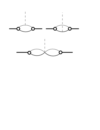
FIG. 13.: Interaction of the graviton with a bound state of two unequal mass particles in the EFT.

As in the scalar EFT, the three diagrams shown in Fig. 13 give the EFT interaction of a graviton with the spin 1/2 bound state described above. [Since the two constituent particles have different properties, the single diagram 12(a) now becomes the first two diagrams shown in Fig. 13.] In the limit when $q\rightarrow 0$, the bound state mass can be obtained from

$$\eta_{\mu\nu}{\cal J}_{M_{b}}^{\mu\nu}(p,p)= -{\bar{\cal U}}(p)\left[M_{b}+S^{-1}_{M_{b}}(p)\right]{\cal U}(p)=$$ (117)

$$= -M_{b}\,{\bar{\cal U}}(p){\cal U}(p)=-M_{b}\,.$$ (118)

Using the relation (91) and the similar relation

$$S_{m_{1}}(k)\,\eta_{\mu\nu}{\cal J}_{m_{1}}^{\mu\nu}(k,k)\,S_{m_{1}}(k)=-m_{1}\,S^{2}_{m_{1}}(k)-S_{m_{1}}(k)=\left(m_{1}\frac{d}{dm_{1}}-1\right)S_{m_{1}}(k)\,,$$ (119)

the first two Feynman diagrams in Fig. 13 become, as $q\rightarrow 0$,

$$\eta_{\mu\nu}{\cal J}_{1+2}^{\mu\nu}(p,p)= -i{\bar{\cal U}}(p){\cal N}^{2}\int\frac{d^{d}k}{(2\pi)^{d}}\Bigl{\{}\Delta_{m_{2}}(p-k)\left(m_{1}\frac{d}{dm_{1}}-1\right)S_{m_{1}}(k)$$ (121)

$$\qquad+S_{m_{1}}(p-k)\,2m_{2}^{2}\frac{d}{dm_{2}^{2}}\Delta_{m_{2}}(k)\Bigr{\}}{{\cal U}}(p)$$

$$= -{\bar{\cal U}}(p){\cal N}^{2}\left(-1+m_{1}\frac{\partial}{\partial m_{1}}+2m_{2}^{2}\frac{\partial}{\partial m_{2}^{2}}\right)\left(A(M_{b}^{2})+\not{p}B(M_{b}^{2})\right){\bar{\cal U}}(p)$$ (122)

$$= -{\cal N}^{2}\left(-1+m_{1}\frac{\partial}{\partial m_{1}}+2m_{2}^{2}\frac{\partial}{\partial m_{2}^{2}}\right)\left(A(M_{b}^{2})+M_{b}B(M_{b}^{2})\right)\,.$$ (123)

As in the scalar case, the third diagram becomes

$$\eta_{\mu\nu}{\cal J}_{3}^{\mu\nu}(p,p)= -2\lambda{\cal N}^{2}{\bar{\cal U}}(p)\left(A(M_{b}^{2})+\not{p}B(M_{b}^{2})\right)^{2}{{\cal U}}(p)$$ (124)

$$= -2\lambda{\cal N}^{2}\left(A(M_{b}^{2})+M_{b}B(M_{b}^{2})\right)^{2}=-2{\cal N}^{2}\left(A(M_{b}^{2})+M_{b}B(M_{b}^{2})\right)\,,$$ (125)

where Eq. (101) was used in the last step. Adding (123) and (125) and equating them to (118) gives the following relation

$$M_{b}={\cal N}^{2}\left(1+m_{1}\frac{\partial}{\partial m_{1}}+2m_{2}^{2}\frac{\partial}{\partial m_{2}^{2}}\right)\left(A(M_{b}^{2})+M_{b}B(M_{b}^{2})\right)\,.$$ (126)

Substituting the expressions (100) for $A$ and $B$ into this equation, and using the identity (104), transforms the equation into

$$M_{b}=\frac{{\cal N}^{2}}{4\pi}\int^{1}_{0}\frac{M_{b}\,x\left[M_{b}(1-x)+m_{1}\right]^{2}dx}{\left[m_{1}^{2}x+m_{2}^{2}(1-x)-M_{b}^{2}x(1-x)\right]^{2}}\,$$ (127)

which is Eq. (105). Consequently the bound state normalization condititon insures the conservation of energy-momentum in this example as well.

V CONCLUSIONs

We have shown for two specific examples in 1+1 dimension that the bound state normalization condition and the energy-momentum conservation condition are, in fact, identical constraints. Similarily, it has been shown[1] for the same systems (and it is true in general) that the normalization condition and charge conservation (or baryon conservation) are also equivalent. For systems with no conserved vector current (charge or baryon number) the conservation of the energy-momentum tensor current associated with gravity may be of special significance.

While our discussion did not apply to higher dimensions, where form factors or cutoffs are needed to regularize the EFT, we conjecture that energy-momentum conservation and the bound state normalization condition must also be equivalent in these cases.

We conclude this paper by returning to our opening discussion of momentum conservation in DIS. While the interaction of a graviton with a bound state would seem to be unrelated to DIS, our proof of energy-momentum conservation ought to imply that the covariant discription of DIS conserves momentum. In fact, for the two body bound states in 1+1 dimension that we have been discussing, the demonstration is very simple.

In the scalar model investigated in Ref. [1], the bound state consisted of a charged particle of mass $m_{1}$ and a neutral particle of mass $m_{2}$. The charge distribution function is

$$f(x)=\frac{{\cal N}^{2}}{4\pi}\frac{x(1-x)}{\left[m_{1}^{2}x+m_{2}^{2}(1-x)-M^{2}\,x(1-x)\right]^{2}}\,,$$ (128)

and charge conservation (and the bound state normalization condition) lead to the requirement that

$$\int_{0}^{1}dxf(x)=1\,.$$ (129)

Note that the distribution amplitude (128) is symmetric under the interchange of $x\to 1=x$ and $m_{1}\to m_{2}$, so that if both $m_{1}$ and $m_{2}$ were charged, we could define two “flavor” distributions

$$f_{1}(x)= f(x)$$ (130)

$$f_{2}(x)= f(1-x)$$ (131)

both normalized to unity. This would insure charge or baryon number conservation

$$b_{1}\int_{0}^{1}dxf_{1}(x)+b_{2}\int_{0}^{1}dxf_{2}(x)=b_{1}+b_{2}$$ (132)

as in Eq. (1). Note that these conditions also insure that momentum is conserved. In this notation, Eq. (2) is written

$$\int_{0}^{1}dx\,xf_{1}(x)+\int_{0}^{1}dx\,xf_{2}(x)=\int_{0}^{1}dx\,xf_{1}(x)+\int_{0}^{1}dx\,(1-x)f_{1}(x)=1$$ (133)

in complete agreement with Eq. (2). We conclude that momentum is conserved in covariant models of DIS.

VI acknowledgments

This research has been supported in part by the DOE under grant No. DE-FG02-97ER41032, and by DOE contract DE-AC05-84ER40150 administered by SURA in support of the Thomas Jefferson National Accelerator Facility. One of us (Z.B.) is a recipient of the graduate fellowship awarded by SURA and the Thomas Jefferson National Accelerator Facility. Support provided by the DOE and the SURA fellowship are gratefully acknowledged. One of us (F.G.) wishes to acknowledge interesting conversations on this topic with Geoffrey West at the Institute for Nuclear Theory, Seattle Washington.

REFERENCES

- [1] Z. Batiz and F. Gross, Phys. Rev. C58, 2963 (1998).
- [2] S. Weinberg, (Wiley, New York, 1972).
- [3] M. Kaku, , (Oxford University Press, 1993).
- [4] H. Ohanian, R. Ruffini, (Norton, New York, 1994).
- [5] F. Gross and D. O. Riska, Phys. Rev. C 36, 1928 (1987).
- [6] R. P. Feynman, Acta Phys. Polon., 24, 697 (1963).
- [7] G. West, unpublished (1991).
- [8] Ç. Şavklı, PhD. Dissertation, Univ. of Pittsburgh (1996).
- [9] M. E. Peskin, D. V. Schroeder, (Addison-Wesley, Reading MA, 1997).
- [10] T. W. B. Kibble, Journal of Math. Phys., 4, 1433 (1963).