Dynamical Test of Constituent Quark Models with $\pi N$ Reactions

Abstract

A dynamical approach is developed to predict the $\pi N$ scattering amplitudes starting with the constituent quark models. The first step is to apply a variational method to solve the three-quark bound state problem. The resulting wave functions are used to calculate the $N^{*}\rightarrow\pi N,\eta N,\pi\Delta$ vertex functions by assuming that the $\pi$ and $\eta$ mesons couple directly to quarks. These vertex functions and the predicted baryon bare masses then define a Hamiltonian for $\pi N$ reactions. We apply a unitary transformation method to derive from the constructed Hamiltonian a multi-channel and multi-resonance reaction model for predicting the $\pi N$ scattering amplitudes up to $W=2$ GeV. With the parameters constrained by the $\Delta(1232$) excitation, we have examined the extent to which the $\pi N$ scattering in $S_{11}$ channel can be described by the constituent quark models based on the one-gluon-exchange or one-meson-exchange mechanisms. It is found that the data seem to favor the spin-spin interaction due to one-meson-exchange and the tensor interaction due to one-gluon-exchange. A phenomenological quark-quark potential has been constructed to reproduce the $S_{11}$ amplitude.

I INTRODUCTION

The constituent quark models have long been used to investigate the structure of nucleon resonances. Most of the earlier works[1, 2, 3, 4] were based on phenomenological forms of residual quark-quark ($qq$) interactions. With the development of Quantum Chromodynamics(QCD), a more fundamental approach was developed[5, 6, 7] by assuming that the residual $qq$ interactions can be parameterized as the Fermi-Breit form of one-gluon-exchange mechanism[8]. In recent years, an alternative approach has been developed[9, 10, 11] based on the assumption that the residual $qq$-interaction is due to the exchange of octet Goldstone bosons. With appropriate phenomenological tuning, both approaches can reproduce the general structure of the baryon spectra listed by Particle Data Group (PDG)[12]. Some attempts[13, 14, 15] have also been made to develop hybrid models including both one-gluon-exchange and one-meson-exchange quark-quark interactions. To make progress, it is important to develop an approach to distinguish all of these constituent quark models using additional experimental data.

The main question we want to address in this work is how the constituent quark models can be tested against the $\pi N$ scattering data. It is common to compare their predicted masses and decay widths with the data listed by PDG. All calculations of decay widths have been done[16, 17, 18, 19, 20, 21] perturbatively. For example, the width of the decay of $N^{*}$ into a $\pi N$ state is calculated by evaluating the matrix element $\langle N^{*}|O(k)|N\rangle$ with an appropriate operator $O(k)$ describing how pions are coupled to quarks. The interactions between the outgoing mesons and baryons are neglected. It has been found that such a perturbative calculation can at best describe the general qualitative trend of the data, but not the quantitative details. For example, the widths of $N(1535)\rightarrow\pi N,\eta N,\pi\Delta$ predicted by Ref.[20] are ($14.7\pm 0.5,14.6\pm 0.4,1.4\pm 0.3$) MeV^1/2 , which do not seem in quantitative agreement with the empirical values ($8.0\pm 2.8,8.1\pm 0.8,0.$) MeV^1/2 determined in Ref.[22].

It is important to note here that the PDG’s values are extracted from the experimental $\pi N$ amplitudes which contain both resonant and non-resonant components. In most partial waves, the non-resonant mechanisms are important ; one can see this from the fact that most of the resonances identified by PDG are in fact not visible in $\pi N$ and $\gamma N$ cross section data. By the unitarity condition, therefore the extracted resonance parameters ”inherently” contain non-resonant contributions. Furthermore, the separation of non-resonant components from the full amplitudes is a model-dependent procedure. The available amplitude analyses[22, 23, 24, 25, 26, 27] have yielded very different resonance parameters in many cases. Clearly, except in a region where the non-resonant contributions are negligibly small, the comparison of the PDG values (or values from other amplitude analyses) with the decay widths calculated perturbatively from the constituent quark models could be very misleading. In particular, a perturbative calculation of decay widths is obviously not valid for cases in which two nearby resonances in the same partial wave can couple with each other through their coupling with the meson-nucleon continuum. Similar precautions must also be taken in comparing the predicted masses with the PDG values. These issues concerning the comparison of the PDG data with the predictions from constituent quark models were discussed in Ref.[28].

To have a more direct test of constituent quark models, we will explore in this work a nonperturbative approach that takes account of the unitarity condition and can relate the $\pi N$ scattering amplitudes directly to the predicted internal quark wave functions of baryons. Our approach is guided by a dynamical model of $\pi N$ and $\gamma N$ reactions developed in Ref.[29] (SL model). It was shown there that the $\pi N$ and $\gamma N$ reactions up to the $\Delta(1232)$ energy region can be described by the following Hamiltonian

$$H=H_{0}+\Gamma_{\Delta\leftrightarrow\pi N,\gamma N}+v_{\pi N,\pi N}+v_{\pi N,\gamma N}\,,$$ (1)

where $\Gamma_{\Delta\rightarrow\pi N,\gamma N}$ describes the $\Delta\leftrightarrow\pi N,\gamma N$ transitions, and $v_{\alpha,\beta}$ are the non-resonant interactions. It was found that the unitarity condition and the non-resonant interaction $v_{\alpha,\beta}$ can shift the mass of $\Delta$ by about 60 MeV and account for as much as about 40 $\%$ of the M1 strength of the $\Delta\rightarrow\gamma N$ decay. This provides an explanation of a long-standing discrepancy between the M1 value predicted by the constituent quark model and the PDG value. It is therefore natural to conjecture that $H_{0}$ of Eq. (1) can be identified with the model Hamiltonian of a constituent quark model, and $\Gamma_{\Delta\rightarrow\pi N,\gamma N}$ correspond to the decay amplitudes calculated perturbatively using the resulting baryon wave functions. This assumption is then similar to what was used in a dynamical study[30] of the $\pi N$ scattering amplitude in $S_{11}$ channel within a constituent quark model. However, Ref.[30] did not consider the non-resonant interaction $v_{\alpha,\beta}$ and employed very simple internal wave functions for the $N^{*}(S_{11})$ states. In this work, we will extend the Hamiltonian Eq. (1) to consider the multi-channel and multi-resonance cases. As a first step, we will focus on the $S_{11}$ channel. We will concentrate on analyzing the dynamical content of our approach in this rather complex channel.

There have been some attempts to understand the constituent quark models within QCD. Manohar and Georgi[31] argued that in the kinematic region between the chiral symmetry breaking scale $\Lambda_{\chi{\rm SB}}\sim 1$ GeV and the QCD confinement scale $\Lambda_{\rm QCD}\sim 0.1-0.3$ GeV, the effective theory for hadrons is defined by the Lagrangian

$$L(g,G,\phi)=\bar{\psi}(i\partial^{\mu}\gamma_{\mu}-m_{q})\psi-ig\bar{\psi}G^{\mu}\gamma_{\mu}\psi-\frac{g_{A}}{2f}\bar{\psi}\gamma^{\mu}\gamma_{5}\psi\partial_{\mu}\phi+\cdot\cdot\cdot\cdot$$ (2)

where $m_{q}$ is the constituent quark mass, $\psi$, $G^{\mu}$, and $\phi$ are the fields for constituent quarks , gluons, and Goldstone bosons, respectively. The most crucial dynamical assumption of this approach is that the Goldstone bosons are coupled directly to the constituent quarks by the flavor SU(3) symmetry characterized by the coupling constant $g_{A}/(2f)$. This is consistent with the notion that the Goldstone bosons result from the spontaneously breaking of the approximate chiral symmetry that characterizes the QCD Lagrangian.

The Lagrangian Eq. (2) implies that the constituent quarks could interact with each other through both the exchanges of gluons and Goldstone bosons. The usual one-gluon-exchange (OGE) and one-meson-exchange (OME) $qq$-interaction can be calculated from Eq. (2) using perturbation theory. This conjecture is supported by a recent Lattice QCD calculation[32]. In Ref.[32], it was found that the mass splitting between $N$ and $\Delta$ is largely due to the meson-exchange mechanism. The need of both flavor-independent (i.e. OGE) and flavor-dependent (i.e. OME) $qq$-interactions is also suggested by the baryon mass formula determined in an algebraic approach[21]. In this work, we will take this point of view and will consider a general constituent quark model which can have both OGE and OME mechanisms. This model can be reduced to the previously developed OGE or OME models in some limits.

The meson-quark couplings were also included in other hadron models such as the chiral/cloudy bag models[33]. However the Lagrangian Eq. (2) with $m_{q}\sim 200-300$ MeV for up and down quarks is closest to a framework within which one can hope to understand the dynamical origins of the most often used constituent quark models based on $qq$-potentials. Perhaps one can apply the dynamical approach developed in this work to also examine other hadron models. But this is beyond the scope of this paper.

In section II, we present the model Hamiltonian for baryons and our method for solving the three-quark bound state problem. The calculations of meson-baryon-baryon vertex functions are given in section III. A formalism for $\pi N$ reactions is developed in section IV. In section V, we analyze the dynamical content of our approach within a simple model. The results and discussions are presented in section VI. Section VII is devoted to conclusions and discussions on future developments.

II INTERNAL STRUCTURE OF BARYONS

A Baryon Hamiltonian

In this exploratory study, we take the simplest, but often used, approach and assume that the baryon structure can be described in terms of three nonrelativistic constituent quarks. The model Hamiltonian is of the following familiar form

$$h_{B}=K+V_{\rm conf}+V_{qq}\ .$$ (3)

The kinetic energy $K$ is defined by

$$K=\sum_{i=1}^{3}\frac{\mathchoice{{\hbox{\boldmath$\displaystyle p$}}}{{\hbox{\boldmath$\textstyle p$}}}{{\hbox{\boldmath$\scriptstyle p$}}}{{\hbox{\boldmath$\scriptscriptstyle p$}}}^{2}_{i}}{2m_{q}}+3m_{q}-\frac{\mathchoice{{\hbox{\boldmath$\displaystyle P$}}}{{\hbox{\boldmath$\textstyle P$}}}{{\hbox{\boldmath$\scriptstyle P$}}}{{\hbox{\boldmath$\scriptscriptstyle P$}}}^{2}}{6m_{q}}\ ,$$ (4)

where $\mathchoice{{\hbox{\boldmath$\displaystyle p$}}}{{\hbox{\boldmath$\textstyle p$}}}{{\hbox{\boldmath$\scriptstyle p$}}}{{\hbox{\boldmath$\scriptscriptstyle p$}}}_{i}$ is the momentum of the $i$th quark and $\textstyle P$ is the center of mass momentum of the three-quark system. The constituent quark mass $m_{q}$ is taken to be 340 MeV, which is close to the value used for describing the nucleon magnetic moments within the simple $(0s)^{3}$ configuration. The confinement potential $V_{\rm conf}$ is assumed to be of the usual linear form

$$V_{\rm conf} = \sum_{i<j}\alpha_{c}r_{ij}\ ,$$ (5)

where $r_{ij}=|\mathchoice{{\hbox{\boldmath$\displaystyle r$}}}{{\hbox{\boldmath$\textstyle r$}}}{{\hbox{\boldmath$\scriptstyle r$}}}{{\hbox{\boldmath$\scriptscriptstyle r$}}}_{i}-\mathchoice{{\hbox{\boldmath$\displaystyle r$}}}{{\hbox{\boldmath$\textstyle r$}}}{{\hbox{\boldmath$\scriptstyle r$}}}{{\hbox{\boldmath$\scriptscriptstyle r$}}}_{j}|$ and $\alpha_{c}$ is a constant.

For the residual $qq$-interaction $V_{qq}$ in Eq. (3), we first consider the cases that either the one-gluon-exchange(OGE) model or the one-meson-exchange(OME) model is used. Both models are derived from taking the static limits of the one-particle-exchange Feynman amplitudes. For the OGE model, following the previous works, we drop its spin-orbit component and retain only spin-spin and tensor components. The OME model has the same structure except that it contains a flavor (isospin) dependent factor $\mathchoice{{\hbox{\boldmath$\displaystyle\tau$}}}{{\hbox{\boldmath$\textstyle\tau$}}}{{\hbox{\boldmath$\scriptstyle\tau$}}}{{\hbox{\boldmath$\scriptscriptstyle\tau$}}}_{i}\cdot\mathchoice{{\hbox{\boldmath$\displaystyle\tau$}}}{{\hbox{\boldmath$\textstyle\tau$}}}{{\hbox{\boldmath$\scriptstyle\tau$}}}{{\hbox{\boldmath$\scriptscriptstyle\tau$}}}_{j}$. We thus consider the following general form of $V_{qq}$

$$V_{qq} = \sum_{i<j}\left[\mathchoice{{\hbox{\boldmath$\displaystyle\sigma$}}}{{\hbox{\boldmath$\textstyle\sigma$}}}{{\hbox{\boldmath$\scriptstyle\sigma$}}}{{\hbox{\boldmath$\scriptscriptstyle\sigma$}}}_{i}\cdot\mathchoice{{\hbox{\boldmath$\displaystyle\sigma$}}}{{\hbox{\boldmath$\textstyle\sigma$}}}{{\hbox{\boldmath$\scriptstyle\sigma$}}}{{\hbox{\boldmath$\scriptscriptstyle\sigma$}}}_{j}V_{\sigma}(r_{ij})+\mathchoice{{\hbox{\boldmath$\displaystyle\sigma$}}}{{\hbox{\boldmath$\textstyle\sigma$}}}{{\hbox{\boldmath$\scriptstyle\sigma$}}}{{\hbox{\boldmath$\scriptscriptstyle\sigma$}}}_{i}\cdot\mathchoice{{\hbox{\boldmath$\displaystyle\sigma$}}}{{\hbox{\boldmath$\textstyle\sigma$}}}{{\hbox{\boldmath$\scriptstyle\sigma$}}}{{\hbox{\boldmath$\scriptscriptstyle\sigma$}}}_{j}\mathchoice{{\hbox{\boldmath$\displaystyle\tau$}}}{{\hbox{\boldmath$\textstyle\tau$}}}{{\hbox{\boldmath$\scriptstyle\tau$}}}{{\hbox{\boldmath$\scriptscriptstyle\tau$}}}_{i}\cdot\mathchoice{{\hbox{\boldmath$\displaystyle\tau$}}}{{\hbox{\boldmath$\textstyle\tau$}}}{{\hbox{\boldmath$\scriptstyle\tau$}}}{{\hbox{\boldmath$\scriptscriptstyle\tau$}}}_{j}V_{\sigma\tau}(r_{ij})+S_{ij}V_{T}(r_{ij})+S_{ij}\mathchoice{{\hbox{\boldmath$\displaystyle\tau$}}}{{\hbox{\boldmath$\textstyle\tau$}}}{{\hbox{\boldmath$\scriptstyle\tau$}}}{{\hbox{\boldmath$\scriptscriptstyle\tau$}}}_{i}\cdot\mathchoice{{\hbox{\boldmath$\displaystyle\tau$}}}{{\hbox{\boldmath$\textstyle\tau$}}}{{\hbox{\boldmath$\scriptstyle\tau$}}}{{\hbox{\boldmath$\scriptscriptstyle\tau$}}}_{j}V_{T\tau}(r_{ij})\right]\ ,$$ (6)

with

$$S_{ij}=\mathchoice{{\hbox{\boldmath$\displaystyle\sigma$}}}{{\hbox{\boldmath$\textstyle\sigma$}}}{{\hbox{\boldmath$\scriptstyle\sigma$}}}{{\hbox{\boldmath$\scriptscriptstyle\sigma$}}}_{i}\cdot\hat{r}_{ij}\mathchoice{{\hbox{\boldmath$\displaystyle\sigma$}}}{{\hbox{\boldmath$\textstyle\sigma$}}}{{\hbox{\boldmath$\scriptstyle\sigma$}}}{{\hbox{\boldmath$\scriptscriptstyle\sigma$}}}_{j}\cdot\hat{r}_{ij}-\frac{1}{3}\mathchoice{{\hbox{\boldmath$\displaystyle\sigma$}}}{{\hbox{\boldmath$\textstyle\sigma$}}}{{\hbox{\boldmath$\scriptstyle\sigma$}}}{{\hbox{\boldmath$\scriptscriptstyle\sigma$}}}_{i}\cdot\mathchoice{{\hbox{\boldmath$\displaystyle\sigma$}}}{{\hbox{\boldmath$\textstyle\sigma$}}}{{\hbox{\boldmath$\scriptstyle\sigma$}}}{{\hbox{\boldmath$\scriptscriptstyle\sigma$}}}_{j}\ .$$ (7)

Here, $\mathchoice{{\hbox{\boldmath$\displaystyle\sigma$}}}{{\hbox{\boldmath$\textstyle\sigma$}}}{{\hbox{\boldmath$\scriptstyle\sigma$}}}{{\hbox{\boldmath$\scriptscriptstyle\sigma$}}}_{i}$ and $\mathchoice{{\hbox{\boldmath$\displaystyle\tau$}}}{{\hbox{\boldmath$\textstyle\tau$}}}{{\hbox{\boldmath$\scriptstyle\tau$}}}{{\hbox{\boldmath$\scriptscriptstyle\tau$}}}_{i}$ are respectively the spin and isospin operators for the $i$th quark. The radial parts of the potentials in Eq. (6) are defined by the momentum space potentials

$$V_{i}(r) = \int\frac{dqq^{2}}{2\pi^{2}}j_{0}(qr)\tilde{V}_{i}(q)\$$ (8)

for $i=\sigma,\sigma\tau$, and

$$V_{i}(r) = \int\frac{dqq^{2}}{2\pi^{2}}j_{2}(qr)\tilde{V}_{i}(q)\$$ (9)

for $i=T,T\tau$. The differences between the OGE model and OME model are in the choices of $\tilde{V}_{i}(q)$ for evaluating Eqs. (8)-(9).

1 OGE Model

The OGE model is obtained by taking

$$\tilde{V}_{\sigma}(q) = -\frac{4\pi\alpha_{s}}{4}\langle\lambda_{i}\cdot\lambda_{j}\rangle\frac{1}{6m_{q}^{2}}F_{\rm g}(q)\ ,$$ (10)

$$\tilde{V}_{T}(q) = -\frac{4\pi\alpha_{s}}{4}\langle\lambda_{i}\cdot\lambda_{j}\rangle\frac{1}{4m_{q}^{2}}F_{\rm g}(q)\ ,$$ (11)

$$\tilde{V}_{\sigma\tau}(q) = 0\ ,$$ (12)

$$\tilde{V}_{T\tau}(q) = 0\ ,$$ (13)

where $\lambda_{i}$ is the color SU(3) generator with

$$\langle\lambda_{1}\cdot\lambda_{2}\rangle=-\frac{8}{3}\ ,$$ (14)

for color singlet baryons considered here, and $\alpha_{s}$ is the quark-gluon coupling constant. In Eqs. (10)-(11), we have introduced a form factor of the form

$$F_{\rm g}(q)=\frac{\Lambda_{\rm g}^{2}}{\Lambda_{\rm g}^{2}+\mathchoice{{\hbox{\boldmath$\displaystyle q$}}}{{\hbox{\boldmath$\textstyle q$}}}{{\hbox{\boldmath$\scriptstyle q$}}}{{\hbox{\boldmath$\scriptscriptstyle q$}}}^{2}}\$$ (15)

to regularize the interactions at short distances. This is consistent with the notion that the constituent quarks are not point particles within an effective theory. This regularization of the $qq$-potential is essential in obtaining convergent solutions for the bound state problem defined by the Hamiltonian $h_{B}$ (Eq. (3)). If the potentials are not regularized by form factors, the ground state energy is not bound from below.

2 OME Model

Since we only consider baryons with strangeness $S=0$, the OME model is defined only by the exchange of $\pi$ and $\eta$ mesons. Because $\eta$ is isospin singlet, it only contributes to the isospin independent parts of the potential. On the other hand, the exchange of the isovector pion leads to isospin dependent terms. The resulting OME model is defined by

$$\tilde{V}_{\sigma}(q) = -\left(\frac{f_{\eta qq}}{m_{\eta}}\right)^{2}\frac{1}{3}\frac{\mathchoice{{\hbox{\boldmath$\displaystyle q$}}}{{\hbox{\boldmath$\textstyle q$}}}{{\hbox{\boldmath$\scriptstyle q$}}}{{\hbox{\boldmath$\scriptscriptstyle q$}}}^{2}}{\mathchoice{{\hbox{\boldmath$\displaystyle q$}}}{{\hbox{\boldmath$\textstyle q$}}}{{\hbox{\boldmath$\scriptstyle q$}}}{{\hbox{\boldmath$\scriptscriptstyle q$}}}^{2}+m_{\eta}^{2}}F_{\eta}(q)\ ,$$ (16)

$$\tilde{V}_{T}(q) = \left(\frac{f_{\eta qq}}{m_{\eta}}\right)^{2}\frac{\mathchoice{{\hbox{\boldmath$\displaystyle q$}}}{{\hbox{\boldmath$\textstyle q$}}}{{\hbox{\boldmath$\scriptstyle q$}}}{{\hbox{\boldmath$\scriptscriptstyle q$}}}^{2}}{\mathchoice{{\hbox{\boldmath$\displaystyle q$}}}{{\hbox{\boldmath$\textstyle q$}}}{{\hbox{\boldmath$\scriptstyle q$}}}{{\hbox{\boldmath$\scriptscriptstyle q$}}}^{2}+m_{\eta}^{2}}F_{\eta}(q)\ ,$$ (17)

$$\tilde{V}_{\sigma\tau}(q) = -\left(\frac{f_{\pi qq}}{m_{\pi}}\right)^{2}\frac{1}{3}\frac{\mathchoice{{\hbox{\boldmath$\displaystyle q$}}}{{\hbox{\boldmath$\textstyle q$}}}{{\hbox{\boldmath$\scriptstyle q$}}}{{\hbox{\boldmath$\scriptscriptstyle q$}}}^{2}}{\mathchoice{{\hbox{\boldmath$\displaystyle q$}}}{{\hbox{\boldmath$\textstyle q$}}}{{\hbox{\boldmath$\scriptstyle q$}}}{{\hbox{\boldmath$\scriptscriptstyle q$}}}^{2}+m_{\pi}^{2}}F_{\pi}(q)\ ,$$ (18)

$$\tilde{V}_{T\tau}(q) = \left(\frac{f_{\pi qq}}{m_{\pi}}\right)^{2}\frac{\mathchoice{{\hbox{\boldmath$\displaystyle q$}}}{{\hbox{\boldmath$\textstyle q$}}}{{\hbox{\boldmath$\scriptstyle q$}}}{{\hbox{\boldmath$\scriptscriptstyle q$}}}^{2}}{\mathchoice{{\hbox{\boldmath$\displaystyle q$}}}{{\hbox{\boldmath$\textstyle q$}}}{{\hbox{\boldmath$\scriptstyle q$}}}{{\hbox{\boldmath$\scriptscriptstyle q$}}}^{2}+m_{\pi}^{2}}F_{\pi}(q)\ ,$$ (19)

where $f_{Mqq}$ is the meson-quark coupling constant, $m_{M}$ denotes the meson mass. Here, as in the OGE model, we introduce a form factor

$$F_{M}(q)=\frac{\Lambda^{2}_{M}}{\Lambda^{2}_{M}+\mathchoice{{\hbox{\boldmath$\displaystyle q$}}}{{\hbox{\boldmath$\textstyle q$}}}{{\hbox{\boldmath$\scriptstyle q$}}}{{\hbox{\boldmath$\scriptscriptstyle q$}}}^{2}}\$$ (20)

to regularize the potentials at short distances.

If we assume that the $\pi NN$ vertex function can be calculated from the $\pi qq$ interaction (as defined later in section III), the $\pi$-quark coupling constant $f_{\pi qq}$ can be related to the $\pi NN$ coupling constant. Within the naive $(0s)^{3}$ configuration for the nucleon, one finds that

$$\frac{f_{\pi qq}}{m_{\pi}}=\frac{3}{5}\frac{g_{\pi NN}}{2M_{N}}\ ,$$ (21)

where $M_{N}$ is the observed mass of the nucleon and we use the empirical value $g_{\pi NN}^{2}/4\pi=14$. The coupling constant $f_{\eta qq}$ can be calculated from $f_{\pi qq}$ by using the flavor SU(3) symmetry,

$$\frac{f_{\eta qq}}{m_{\eta}}=\frac{1}{\sqrt{3}}\frac{f_{\pi qq}}{m_{\pi}}\ .$$ (22)

Since there may be SU(3) symmetry breaking mechanisms, the coupling constant $f_{\eta qq}$ could be different from its SU(3) value. We however do not consider this possibility in defining the OME model and simply use Eq. (22).

B Solution of three-quark bound state problem

With the Hamiltonian $h_{B}$ (Eq. (3)) defined above, our first task is to solve the following three-body bound state problem in the $\mathchoice{{\hbox{\boldmath$\displaystyle P$}}}{{\hbox{\boldmath$\textstyle P$}}}{{\hbox{\boldmath$\scriptstyle P$}}}{{\hbox{\boldmath$\scriptscriptstyle P$}}}=0$ rest frame of the system

$$h_{B}|\Psi^{B}\rangle=m_{B}|\Psi^{B}\rangle\ ,$$ (23)

where $|\Psi^{B}\rangle$ is the baryon wave function with the label $B$ denoting collectively the spin-parity $J^{\pi}$ and isospin $T$ ; $m_{B}$ is the mass eigenvalue. We use the diagonalization method developed in Ref.[34] to solve Eq. (23). The basis states for the diagonalization are formed from harmonic oscillator wave functions. This choice has two advantages: (1) By using appropriate Jacobi coordinates, the center of mass motion can be separated exactly from the intrinsic wave functions, (2) The resulting wave functions have the desired S₃ symmetry.

In the diagonalization method, the baryon wave function is expanded as

$$|\Psi^{J^{\pi}T}\rangle=\sum_{i}a^{J^{\pi}T}_{i}|J^{\pi}T;i\rangle,$$ (24)

where the basis wave functions are of the following antisymmetrized form:

$$|J^{\pi}T;i\rangle=\sum_{\alpha}c_{\alpha}^{i}\left[|\phi_{NL}^{\alpha_{\rm space}}\rangle\otimes|\chi_{S}^{\alpha_{\rm spin}}\rangle\right]_{(J)}\cdot|\eta_{T}^{\alpha_{\rm flavor}}\rangle\cdot|\varphi^{\rm A}\rangle\ .$$ (25)

Here $\alpha=\{\alpha_{\rm space},\alpha_{\rm spin},\alpha_{\rm flavor}\}$ stands for the S₃ symmetry of each part of the wave function. $|\phi_{NL}^{\alpha_{\rm space}}\rangle$ and $|\chi_{S}^{\alpha_{\rm spin}}\rangle$ are the spatial and spin wave functions with the orbital angular momentum $L$, quanta of harmonic oscillator $N$, and spin $S$. They couple to give the total angular momentum $J$ of the baryon. $|\eta_{T}^{\alpha_{\rm flavor}}\rangle$ and $|\varphi^{\rm A}\rangle$ are the iso-spin and color wave functions, respectively. The color wave function $|\varphi^{\rm A}\rangle$ is totally antisymmetric. By taking appropriate coefficients $c_{\alpha}^{i}$, the basis state $|J^{\pi}T;i\rangle$ defined by Eq. (25) is totally antisymmetric.

The coefficients $a^{J^{\pi}T}_{i}$ in Eq. (24) and the mass eigenvalues $m_{J^{\pi}T}$ are obtained from diagonalizing the matrix

$$H_{i,j}=\langle J^{\pi}T;i|h_{B}|J^{\pi}T;j\rangle.$$ (26)

In practice diagonalization is performed within a limited number of basis states. Then the solution of Eq. (23) is a function of the oscillator range parameter $b$. We treat it as a variational parameter and find $b$ by imposing the condition:

$$\frac{\partial m_{B}}{\partial b}=0\ .$$ (27)

The basis state is chosen so that the mass eigenvalue $m_{J^{\pi}T}$ does not change by further extension of the basis states. In practice we include the basis states up to 11$\hbar\omega$.

For later discussions, we write down here the lowest basis wave functions for $N$, $\Delta$, and $N^{*}(S_{11})$ (simply called $N^{*}$ from now on)

$$|\Psi^{N}\rangle \equiv |\frac{1}{2}^{+}\frac{1}{2};1\rangle=\frac{1}{\sqrt{2}}|\phi_{00}^{\rm S}\rangle\left(|\chi_{1/2}^{\rm MS}\rangle|\eta^{\rm MS}_{1/2}\rangle+|\chi^{\rm MA}_{1/2}\rangle|\eta^{\rm MA}_{1/2}\rangle\right)|\varphi^{\rm A}\rangle\ ,$$ (28)

$$|\Psi^{\Delta}\rangle \equiv |\frac{3}{2}^{+}\frac{3}{2};1\rangle=|\phi^{\rm S}_{00}\rangle|\chi_{3/2}^{\rm S}\rangle|\eta^{\rm S}_{3/2}\rangle|\varphi^{\rm A}\rangle\ ,$$ (29)

$$|\Psi^{N^{*}_{1}}S=1/2\rangle \equiv |\frac{1}{2}^{-}\frac{1}{2};1\rangle=\frac{1}{2}\left\{\left[|\phi_{11}^{\rm MS}\rangle\otimes|\chi_{1/2}^{\rm MS}\rangle-|\phi_{11}^{\rm MA}\rangle\otimes|\chi^{\rm MA}_{1/2}\rangle\right]_{(1/2)}|\eta_{1/2}^{\rm MS}\rangle\right.$$ (31)

$$\mbox{}\ \ \ \ \ \ \ \ \ \ \ \ \ \ \ \left.-\left[|\phi_{11}^{\rm MS}\rangle\otimes|\chi_{1/2}^{\rm MA}\rangle+|\phi_{11}^{\rm MA}\rangle\otimes|\chi^{\rm MS}_{1/2}\rangle\right]_{(1/2)}|\eta_{1/2}^{\rm MA}\rangle\right\}|\varphi^{\rm A}\rangle\ ,$$

$$|\Psi^{N^{*}_{2}}S=3/2\rangle \equiv |\frac{1}{2}^{-}\frac{1}{2};2\rangle=\frac{1}{\sqrt{2}}\left\{\left[|\phi^{\rm MS}_{11}\rangle\otimes|\chi^{\rm S}_{3/2}\rangle\right]_{(1/2)}|\eta^{\rm MS}_{1/2}\rangle+\left[|\phi^{\rm MA}_{11}\rangle\otimes|\chi^{\rm S}_{3/2}\rangle\right]_{(1/2)}|\eta^{\rm MA}_{1/2}\rangle\right\}|\varphi^{\rm A}\rangle\ ,$$ (32)

where $\phi^{\rm S}_{NL}$ denotes a state which is totally symmetric with respect to the interchange of any pair of quarks, and $\phi^{\rm MS(MA)}_{NL}$ denote states with mixed symmetries. Similar upper indices are also used to specify the symmetry properties of the spin wave function $|\chi\rangle$ and isospin wave function $|\eta\rangle$. The spatial wave function can be explicitly written as

$$\langle\mathchoice{{\hbox{\boldmath$\displaystyle r$}}}{{\hbox{\boldmath$\textstyle r$}}}{{\hbox{\boldmath$\scriptstyle r$}}}{{\hbox{\boldmath$\scriptscriptstyle r$}}},\mathchoice{{\hbox{\boldmath$\displaystyle\rho$}}}{{\hbox{\boldmath$\textstyle\rho$}}}{{\hbox{\boldmath$\scriptstyle\rho$}}}{{\hbox{\boldmath$\scriptscriptstyle\rho$}}}|\phi^{\rm S}_{00}\rangle = [R_{00}(r)Y_{0}(\hat{r})\otimes R_{00}(\rho)Y_{0}(\hat{\rho})]_{(0)}\ ,$$ (33)

$$\langle\mathchoice{{\hbox{\boldmath$\displaystyle r$}}}{{\hbox{\boldmath$\textstyle r$}}}{{\hbox{\boldmath$\scriptstyle r$}}}{{\hbox{\boldmath$\scriptscriptstyle r$}}},\mathchoice{{\hbox{\boldmath$\displaystyle\rho$}}}{{\hbox{\boldmath$\textstyle\rho$}}}{{\hbox{\boldmath$\scriptstyle\rho$}}}{{\hbox{\boldmath$\scriptscriptstyle\rho$}}}|\phi^{\rm MS}_{11}\rangle = -[R_{00}(r)Y_{0}(\hat{r})\otimes R_{01}(\rho)Y_{1}(\hat{\rho})]_{(1)}\ ,$$ (34)

$$\langle\mathchoice{{\hbox{\boldmath$\displaystyle r$}}}{{\hbox{\boldmath$\textstyle r$}}}{{\hbox{\boldmath$\scriptstyle r$}}}{{\hbox{\boldmath$\scriptscriptstyle r$}}},\mathchoice{{\hbox{\boldmath$\displaystyle\rho$}}}{{\hbox{\boldmath$\textstyle\rho$}}}{{\hbox{\boldmath$\scriptstyle\rho$}}}{{\hbox{\boldmath$\scriptscriptstyle\rho$}}}|\phi^{\rm MA}_{11}\rangle = [R_{01}(r)Y_{1}(\hat{r})\otimes R_{00}(\rho)Y_{0}(\hat{\rho})]_{(1)}\ ,$$ (35)

where

$$r = \mathchoice{{\hbox{\boldmath$\displaystyle r$}}}{{\hbox{\boldmath$\textstyle r$}}}{{\hbox{\boldmath$\scriptstyle r$}}}{{\hbox{\boldmath$\scriptscriptstyle r$}}}_{1}-\mathchoice{{\hbox{\boldmath$\displaystyle r$}}}{{\hbox{\boldmath$\textstyle r$}}}{{\hbox{\boldmath$\scriptstyle r$}}}{{\hbox{\boldmath$\scriptscriptstyle r$}}}_{2}\ ,$$ (36)

$$\rho = \mathchoice{{\hbox{\boldmath$\displaystyle r$}}}{{\hbox{\boldmath$\textstyle r$}}}{{\hbox{\boldmath$\scriptstyle r$}}}{{\hbox{\boldmath$\scriptscriptstyle r$}}}_{3}-\frac{\mathchoice{{\hbox{\boldmath$\displaystyle r$}}}{{\hbox{\boldmath$\textstyle r$}}}{{\hbox{\boldmath$\scriptstyle r$}}}{{\hbox{\boldmath$\scriptscriptstyle r$}}}_{1}+\mathchoice{{\hbox{\boldmath$\displaystyle r$}}}{{\hbox{\boldmath$\textstyle r$}}}{{\hbox{\boldmath$\scriptstyle r$}}}{{\hbox{\boldmath$\scriptscriptstyle r$}}}_{2}}{2}\ ,$$ (37)

and $R_{nl}$, $Y_{l}$ are the radial wave function and spherical harmonics respectively. The spin and isospin wave functions in Eqs. (28)-(32) can be constructed by using the well known procedure.

III meson-baryon-baryon vertex functions

Within the constituent quark model, the decay of a baryon ($B$) into a meson-baryon ($M^{\prime}B^{\prime}$) state is determined by the matrix element

$$\Gamma_{B^{\prime}M^{\prime},B}^{\dagger}({\mathchoice{{\hbox{\boldmath$\displaystyle k$}}}{{\hbox{\boldmath$\textstyle k$}}}{{\hbox{\boldmath$\scriptstyle k$}}}{{\hbox{\boldmath$\scriptscriptstyle k$}}}})=\langle\Psi^{B^{\prime}};M^{\prime}|H_{M}({\mathchoice{{\hbox{\boldmath$\displaystyle k$}}}{{\hbox{\boldmath$\textstyle k$}}}{{\hbox{\boldmath$\scriptstyle k$}}}{{\hbox{\boldmath$\scriptscriptstyle k$}}}})|\Psi^{B}\rangle\ ,$$ (38)

where $\Psi^{B}$ is a bound state wave function generated from the above structure calculation, and $H_{M}({\mathchoice{{\hbox{\boldmath$\displaystyle k$}}}{{\hbox{\boldmath$\textstyle k$}}}{{\hbox{\boldmath$\scriptstyle k$}}}{{\hbox{\boldmath$\scriptscriptstyle k$}}}})$ is an appropriate operator describing how a meson $M$ with a momentum $\textstyle k$ is emitted or absorbed by constituent quarks. In most of the previous works[16, 17, 18, 19, 21], one assumes that $H_{M}(\mathchoice{{\hbox{\boldmath$\displaystyle k$}}}{{\hbox{\boldmath$\textstyle k$}}}{{\hbox{\boldmath$\scriptstyle k$}}}{{\hbox{\boldmath$\scriptscriptstyle k$}}})$ is a one-body operator with the parameters determined phenomenologically by fitting some of the partial decay widths listed by PDG. Calculations have also been done[20] by using the ${}^{3}P_{0}$ model for $H_{M}(\mathchoice{{\hbox{\boldmath$\displaystyle k$}}}{{\hbox{\boldmath$\textstyle k$}}}{{\hbox{\boldmath$\scriptstyle k$}}}{{\hbox{\boldmath$\scriptscriptstyle k$}}})$.

In this work we assume that $H_{M}(\mathchoice{{\hbox{\boldmath$\displaystyle k$}}}{{\hbox{\boldmath$\textstyle k$}}}{{\hbox{\boldmath$\scriptstyle k$}}}{{\hbox{\boldmath$\scriptscriptstyle k$}}})$ is a one-body operator which can be derived directly from the effective Lagrangian Eq. (2) by taking the nonrelativistic limit of the Feynman amplitude $\bar{u}_{{\mathchoice{{\hbox{\boldmath$\displaystyle p$}}}{{\hbox{\boldmath$\textstyle p$}}}{{\hbox{\boldmath$\scriptstyle p$}}}{{\hbox{\boldmath$\scriptscriptstyle p$}}}}^{\prime}}\gamma_{5}\gamma^{\mu}k_{\mu}u_{{\mathchoice{{\hbox{\boldmath$\displaystyle p$}}}{{\hbox{\boldmath$\textstyle p$}}}{{\hbox{\boldmath$\scriptstyle p$}}}{{\hbox{\boldmath$\scriptscriptstyle p$}}}}}$ for the $q\leftrightarrow Mq$ transition. To be consistent with the nonrelativistic treatment of constituent quarks, we keep only the terms up to the order of $p/m_{q}$. In coordinate space, the resulting $q+\pi\rightarrow q$ transition operator is

$$H_{\pi qq}=\frac{i}{\sqrt{(2\pi)^{3}2\omega_{\pi}}}\frac{f_{\pi qq}}{m_{\pi}}\sum_{i=1}^{3}e^{i{\mathchoice{{\hbox{\boldmath$\displaystyle k$}}}{{\hbox{\boldmath$\textstyle k$}}}{{\hbox{\boldmath$\scriptstyle k$}}}{{\hbox{\boldmath$\scriptscriptstyle k$}}}}\cdot{\mathchoice{{\hbox{\boldmath$\displaystyle r$}}}{{\hbox{\boldmath$\textstyle r$}}}{{\hbox{\boldmath$\scriptstyle r$}}}{{\hbox{\boldmath$\scriptscriptstyle r$}}}}_{i}}\tau^{\alpha}\mathchoice{{\hbox{\boldmath$\displaystyle\sigma$}}}{{\hbox{\boldmath$\textstyle\sigma$}}}{{\hbox{\boldmath$\scriptstyle\sigma$}}}{{\hbox{\boldmath$\scriptscriptstyle\sigma$}}}_{i}\cdot\left[\mathchoice{{\hbox{\boldmath$\displaystyle k$}}}{{\hbox{\boldmath$\textstyle k$}}}{{\hbox{\boldmath$\scriptstyle k$}}}{{\hbox{\boldmath$\scriptscriptstyle k$}}}-\frac{\omega_{\pi}}{2m_{q}}({\mathchoice{{\hbox{\boldmath$\displaystyle p$}}}{{\hbox{\boldmath$\textstyle p$}}}{{\hbox{\boldmath$\scriptstyle p$}}}{{\hbox{\boldmath$\scriptscriptstyle p$}}}}_{i}+{\mathchoice{{\hbox{\boldmath$\displaystyle p$}}}{{\hbox{\boldmath$\textstyle p$}}}{{\hbox{\boldmath$\scriptstyle p$}}}{{\hbox{\boldmath$\scriptscriptstyle p$}}}}^{\prime}_{i})\right]F(k)\ ,$$ (39)

where $\alpha$ denotes the $z$-component of pion isospin and $\mathchoice{{\hbox{\boldmath$\displaystyle p$}}}{{\hbox{\boldmath$\textstyle p$}}}{{\hbox{\boldmath$\scriptstyle p$}}}{{\hbox{\boldmath$\scriptscriptstyle p$}}}_{i}$ ($\mathchoice{{\hbox{\boldmath$\displaystyle p$}}}{{\hbox{\boldmath$\textstyle p$}}}{{\hbox{\boldmath$\scriptstyle p$}}}{{\hbox{\boldmath$\scriptscriptstyle p$}}}_{i}^{\prime}$) is the derivative operator acting on the initial (final) baryon wave function; $\textstyle k$ and $\omega_{\pi}=\sqrt{m_{\pi}^{2}+\mathchoice{{\hbox{\boldmath$\displaystyle k$}}}{{\hbox{\boldmath$\textstyle k$}}}{{\hbox{\boldmath$\scriptstyle k$}}}{{\hbox{\boldmath$\scriptscriptstyle k$}}}^{2}}$ are the momentum and energy of pion, respectively. The operator $H_{\eta qq}$ for the isoscalar $\eta$ meson can be obtained from Eq. (39) by replacing the label $\pi$ by $\eta$ and dropping the isospin operator $\tau^{\alpha}$.

We note that the operator structure of Eq. (39) is the same as that used in Refs.[18, 21]. In Refs.[18, 21], however the coefficients in front of each term are treated as free parameters. Here the relative importance between these two terms are fixed by the non-relativistic reduction of the effective Lagrangian Eq. (2). To take into account SU(3) breaking, we will allow the parameter $f_{\eta qq}$ to deviate from its SU(3) value given by Eq. (22). Furthermore, we also introduce an additional form factor $F(k)$ to account for the effect due to the finite size of constituent quarks and mesons. This is consistent with the procedure used above in defining the $qq$-potential $V_{qq}$. However, the constituent quark form factor for the interaction Eq. (39) could be different from that for the effective $qq$-potential, since the mesons associated with $H_{\pi qq}$ are time-like whereas those associated with $V_{qq}$ are space-like. The constituent quark form factors used in the meson-quark interactions will be introduced in the section discussing our results.

With the operator Eq. (39), we find that the $M+B_{i}\rightarrow B_{f}$ vertex function can be written as

$$\langle\Psi^{B_{f}}|H_{\pi qq}|\Psi^{B_{i}};M\rangle = \sqrt{4\pi}\sum_{JM}\langle J_{i}JM_{i}M|J_{f}M_{f}\rangle\langle T_{i}TT_{iz}T_{z}|T_{f}T_{fz}\rangle$$ (40)

$$\times i^{J}Y_{JM}^{*}(\hat{q})\Gamma_{B_{f}B_{i}}^{JT}(q)\delta(\mathchoice{{\hbox{\boldmath$\displaystyle p$}}}{{\hbox{\boldmath$\textstyle p$}}}{{\hbox{\boldmath$\scriptstyle p$}}}{{\hbox{\boldmath$\scriptscriptstyle p$}}}_{f}-\mathchoice{{\hbox{\boldmath$\displaystyle p$}}}{{\hbox{\boldmath$\textstyle p$}}}{{\hbox{\boldmath$\scriptstyle p$}}}{{\hbox{\boldmath$\scriptscriptstyle p$}}}_{i}-\mathchoice{{\hbox{\boldmath$\displaystyle k$}}}{{\hbox{\boldmath$\textstyle k$}}}{{\hbox{\boldmath$\scriptstyle k$}}}{{\hbox{\boldmath$\scriptscriptstyle k$}}})\ ,$$ (41)

where $\mathchoice{{\hbox{\boldmath$\displaystyle p$}}}{{\hbox{\boldmath$\textstyle p$}}}{{\hbox{\boldmath$\scriptstyle p$}}}{{\hbox{\boldmath$\scriptscriptstyle p$}}}_{i}$, $J_{i}$ and $T_{i}$ ($\mathchoice{{\hbox{\boldmath$\displaystyle p$}}}{{\hbox{\boldmath$\textstyle p$}}}{{\hbox{\boldmath$\scriptstyle p$}}}{{\hbox{\boldmath$\scriptscriptstyle p$}}}_{f}$, $J_{f}$ and $T_{f}$) are the momentum, spin and isospin of the initial (final) baryon, respectively. Their $z$-components are denoted by $M_{i}$ and $T_{iz}$ ($M_{f}$ and $T_{fz}$). $T$, $T_{Z}$ and $\textstyle k$ are the isospin and momentum of meson $M$ ($\pi$ or $\eta$); $\textstyle q$ is the relative momentum of the initial meson-baryon system. In the center of mass frame (the rest frame of the final baryon $B_{f}$), we obviously have the simplification that $\mathchoice{{\hbox{\boldmath$\displaystyle p$}}}{{\hbox{\boldmath$\textstyle p$}}}{{\hbox{\boldmath$\scriptstyle p$}}}{{\hbox{\boldmath$\scriptscriptstyle p$}}}_{i}=-\mathchoice{{\hbox{\boldmath$\displaystyle k$}}}{{\hbox{\boldmath$\textstyle k$}}}{{\hbox{\boldmath$\scriptstyle k$}}}{{\hbox{\boldmath$\scriptscriptstyle k$}}}$ and $\mathchoice{{\hbox{\boldmath$\displaystyle q$}}}{{\hbox{\boldmath$\textstyle q$}}}{{\hbox{\boldmath$\scriptstyle q$}}}{{\hbox{\boldmath$\scriptscriptstyle q$}}}=\mathchoice{{\hbox{\boldmath$\displaystyle k$}}}{{\hbox{\boldmath$\textstyle k$}}}{{\hbox{\boldmath$\scriptstyle k$}}}{{\hbox{\boldmath$\scriptscriptstyle k$}}}$. $\Gamma_{B_{f}B_{i}}^{JT}(k)$ contains the $k$-dependence of the vertex function

$$\Gamma_{B_{f}B_{i}}^{JT}(k) = \frac{3}{\sqrt{(2\pi)^{3}2\omega_{\pi}}}\frac{f_{Mqq}}{m_{\pi}}\sqrt{4\pi}\sum_{L}\sqrt{\frac{2L+1}{2J+1}}(-1)^{J+L}F(k)$$ (44)

$$\times\left\{-(-i)^{L+1-J}\langle L100|J0\rangle\left(1-\frac{\omega_{M}}{6m_{q}}\right)k\langle B_{f}|||j_{L}(\textstyle{\frac{2}{3}}k\rho)[Y_{L}\otimes\sigma]_{(J)}\tau^{T}|||B_{i}\rangle\right.$$

$$\left.\ \ \ \ \ -\frac{\omega_{M}}{m_{q}}\langle B_{f}|||j_{J}(\textstyle{\frac{2}{3}}k\rho)[[Y_{J}\otimes\nabla]_{(L)}\otimes\sigma]_{(J)}\tau^{T}|||B_{i}\rangle\right\}\ .$$

If the simple wave functions Eqs. (28)-(32) are used to evaluate Eq.(40), we obtain the following analytic expressions for the $\pi N\rightarrow N^{*}_{i}$ vertex functions

$$\Gamma^{01}_{N^{*}_{1}N}(k) = 2\Gamma_{\pi}(k)\ ,$$ (45)

$$\Gamma^{01}_{N^{*}_{2}N}(q) = -\Gamma_{\pi}(k)\ ,$$ (46)

with

$$\Gamma_{\pi}(k) = \frac{4}{\sqrt{3}b}\sqrt{\frac{4\pi}{(2\pi)^{3}2\omega_{\pi}}}\left(\frac{f_{\pi qq}}{m_{\pi}}\right)\left[y+\left(-\frac{1}{2}+\frac{y}{6}\right)\frac{\omega_{\pi}}{m_{q}}\right]\exp(-y)F(k),$$ (47)

where $y=b^{2}k^{2}/12$. Likewise the $\eta N\rightarrow N^{*}_{i}$ vertex functions are found to be

$$\Gamma^{00}_{N^{*}_{1}N}(k)= \Gamma^{00}_{N^{*}_{2}N}(k)=-\Gamma_{\eta}(k).$$ (48)

$\Gamma_{\eta}$ can be obtained from $\Gamma_{\pi}$ defined in Eq.(43) by replacing the label $\pi$ by $\eta$. Note that the relative importance of the decay vertex functions of $N^{*}_{1}$ and $N^{*}_{2}$ is completely determined by the differences in their wave functions given in Eqs. (30)-(31).

IV Dynamical model for $\pi N$ reactions

With the vertex functions defined by Eq. (41), we follow the procedures of the SL model to develop a dynamical model for $\pi N$ reactions. The starting Hamiltonian is assumed to be

$$H=H_{0}+H_{I}\ ,$$ (49)

where the free Hamiltonian takes the following second-quantization form

$$H_{0}=\sum_{B}\int d\mathchoice{{\hbox{\boldmath$\displaystyle p$}}}{{\hbox{\boldmath$\textstyle p$}}}{{\hbox{\boldmath$\scriptstyle p$}}}{{\hbox{\boldmath$\scriptscriptstyle p$}}}\,\varepsilon_{B}(\mathchoice{{\hbox{\boldmath$\displaystyle p$}}}{{\hbox{\boldmath$\textstyle p$}}}{{\hbox{\boldmath$\scriptstyle p$}}}{{\hbox{\boldmath$\scriptscriptstyle p$}}})b^{\dagger}_{B}(\mathchoice{{\hbox{\boldmath$\displaystyle p$}}}{{\hbox{\boldmath$\textstyle p$}}}{{\hbox{\boldmath$\scriptstyle p$}}}{{\hbox{\boldmath$\scriptscriptstyle p$}}})b_{B}(\mathchoice{{\hbox{\boldmath$\displaystyle p$}}}{{\hbox{\boldmath$\textstyle p$}}}{{\hbox{\boldmath$\scriptstyle p$}}}{{\hbox{\boldmath$\scriptscriptstyle p$}}})+\sum_{M}\int d\mathchoice{{\hbox{\boldmath$\displaystyle k$}}}{{\hbox{\boldmath$\textstyle k$}}}{{\hbox{\boldmath$\scriptstyle k$}}}{{\hbox{\boldmath$\scriptscriptstyle k$}}}\,\omega_{M}(\mathchoice{{\hbox{\boldmath$\displaystyle k$}}}{{\hbox{\boldmath$\textstyle k$}}}{{\hbox{\boldmath$\scriptstyle k$}}}{{\hbox{\boldmath$\scriptscriptstyle k$}}})a^{\dagger}_{M}(\mathchoice{{\hbox{\boldmath$\displaystyle k$}}}{{\hbox{\boldmath$\textstyle k$}}}{{\hbox{\boldmath$\scriptstyle k$}}}{{\hbox{\boldmath$\scriptscriptstyle k$}}})a_{M}(\mathchoice{{\hbox{\boldmath$\displaystyle k$}}}{{\hbox{\boldmath$\textstyle k$}}}{{\hbox{\boldmath$\scriptstyle k$}}}{{\hbox{\boldmath$\scriptscriptstyle k$}}})\ .$$ (50)

Here, $b^{\dagger}_{B}$($b_{B}$) and $a^{\dagger}_{M}$($a_{M}$) are the creation (annihilation) operators for the baryons and mesons respectively, and

$$\varepsilon_{B}(\mathchoice{{\hbox{\boldmath$\displaystyle p$}}}{{\hbox{\boldmath$\textstyle p$}}}{{\hbox{\boldmath$\scriptstyle p$}}}{{\hbox{\boldmath$\scriptscriptstyle p$}}}) = \sqrt{m_{B}^{2}+\mathchoice{{\hbox{\boldmath$\displaystyle p$}}}{{\hbox{\boldmath$\textstyle p$}}}{{\hbox{\boldmath$\scriptstyle p$}}}{{\hbox{\boldmath$\scriptscriptstyle p$}}}^{2}}\ ,$$ (51)

$$\omega_{M}(\mathchoice{{\hbox{\boldmath$\displaystyle k$}}}{{\hbox{\boldmath$\textstyle k$}}}{{\hbox{\boldmath$\scriptstyle k$}}}{{\hbox{\boldmath$\scriptscriptstyle k$}}}) = \sqrt{m_{M}^{2}+\mathchoice{{\hbox{\boldmath$\displaystyle k$}}}{{\hbox{\boldmath$\textstyle k$}}}{{\hbox{\boldmath$\scriptstyle k$}}}{{\hbox{\boldmath$\scriptscriptstyle k$}}}^{2}}\ .$$ (52)

The baryon mass $m_{B}$ is generated from the structure calculation described in section II, while we use the experimental value for the meson mass $m_{M}$.

The interaction term in Eq. (49) is written in terms of the vertex functions defined in section III

$$H_{I}=\sum_{BB^{\prime}M}\int d\mathchoice{{\hbox{\boldmath$\displaystyle p$}}}{{\hbox{\boldmath$\textstyle p$}}}{{\hbox{\boldmath$\scriptstyle p$}}}{{\hbox{\boldmath$\scriptscriptstyle p$}}}d\mathchoice{{\hbox{\boldmath$\displaystyle p$}}}{{\hbox{\boldmath$\textstyle p$}}}{{\hbox{\boldmath$\scriptstyle p$}}}{{\hbox{\boldmath$\scriptscriptstyle p$}}}^{\prime}d\mathchoice{{\hbox{\boldmath$\displaystyle k$}}}{{\hbox{\boldmath$\textstyle k$}}}{{\hbox{\boldmath$\scriptstyle k$}}}{{\hbox{\boldmath$\scriptscriptstyle k$}}}\left[\langle\Psi^{B^{\prime}}|H_{Mqq}|\Psi^{B};M\rangle b^{\dagger}_{B^{\prime}}(\mathchoice{{\hbox{\boldmath$\displaystyle p$}}}{{\hbox{\boldmath$\textstyle p$}}}{{\hbox{\boldmath$\scriptstyle p$}}}{{\hbox{\boldmath$\scriptscriptstyle p$}}}^{\prime})b_{B}(\mathchoice{{\hbox{\boldmath$\displaystyle p$}}}{{\hbox{\boldmath$\textstyle p$}}}{{\hbox{\boldmath$\scriptstyle p$}}}{{\hbox{\boldmath$\scriptscriptstyle p$}}})a_{M}(\mathchoice{{\hbox{\boldmath$\displaystyle k$}}}{{\hbox{\boldmath$\textstyle k$}}}{{\hbox{\boldmath$\scriptstyle k$}}}{{\hbox{\boldmath$\scriptscriptstyle k$}}})+\mbox{h.c.}\right].$$ (53)

The above interaction Hamiltonian is similar to that of the SL model, except that the anti-baryon states are absent here. As discussed in Ref.[29], it is a non-trivial many-body problem to calculate $\pi N$ reactions with the use of $H_{I}$. To obtain a manageable reaction theory, we follow Refs.[29, 35] and apply the unitary transformation up to the second order in $H_{I}$ to derive an effective Hamiltonian. The essence of the unitary transformation method applied in Ref.[29] is to absorb the unphysical transition $B\rightarrow M^{\prime}B^{\prime}$ with $m_{B}<m_{B^{\prime}}+m_{M^{\prime}}$ into non-resonant potentials. The resulting effective Hamiltonian then takes the following form

$$H_{\rm eff} = H_{0}+\Gamma+\Gamma^{\dagger}+\hat{v}\ ,$$ (54)

where $H_{0}$ is defined in Eq. (50). The vertex $\Gamma^{\dagger}$ contains only the physical decay process $B\rightarrow M^{\prime}B^{\prime}$ with $m_{B}>m_{M^{\prime}}+m_{B^{\prime}}$

$$\Gamma^{\dagger}=\sum_{MBB^{\prime}}\int d\mathchoice{{\hbox{\boldmath$\displaystyle k$}}}{{\hbox{\boldmath$\textstyle k$}}}{{\hbox{\boldmath$\scriptstyle k$}}}{{\hbox{\boldmath$\scriptscriptstyle k$}}}d\mathchoice{{\hbox{\boldmath$\displaystyle p$}}}{{\hbox{\boldmath$\textstyle p$}}}{{\hbox{\boldmath$\scriptstyle p$}}}{{\hbox{\boldmath$\scriptscriptstyle p$}}}d\mathchoice{{\hbox{\boldmath$\displaystyle p$}}}{{\hbox{\boldmath$\textstyle p$}}}{{\hbox{\boldmath$\scriptstyle p$}}}{{\hbox{\boldmath$\scriptscriptstyle p$}}}^{\prime}\ \langle\Psi^{B^{\prime}};M^{\prime}|H_{Mqq}|\Psi^{B}\rangle b^{\dagger}_{B^{\prime}}(\mathchoice{{\hbox{\boldmath$\displaystyle p$}}}{{\hbox{\boldmath$\textstyle p$}}}{{\hbox{\boldmath$\scriptstyle p$}}}{{\hbox{\boldmath$\scriptscriptstyle p$}}}^{\prime})a^{\dagger}_{M^{\prime}}(\mathchoice{{\hbox{\boldmath$\displaystyle k$}}}{{\hbox{\boldmath$\textstyle k$}}}{{\hbox{\boldmath$\scriptstyle k$}}}{{\hbox{\boldmath$\scriptscriptstyle k$}}}^{\prime})b_{B}(\mathchoice{{\hbox{\boldmath$\displaystyle p$}}}{{\hbox{\boldmath$\textstyle p$}}}{{\hbox{\boldmath$\scriptstyle p$}}}{{\hbox{\boldmath$\scriptscriptstyle p$}}})\theta(m_{B}-(m_{B^{\prime}}+m_{M^{\prime}}))\ .$$ (55)

where $\theta(x)=1(0)$ for $x>0(x<0)$. The non-resonant $MB\rightarrow M^{\prime}B^{\prime}$ two-body interactions are defined by

$$\hat{v}=\sum_{MM^{\prime}BB^{\prime}}\int d\mathchoice{{\hbox{\boldmath$\displaystyle k$}}}{{\hbox{\boldmath$\textstyle k$}}}{{\hbox{\boldmath$\scriptstyle k$}}}{{\hbox{\boldmath$\scriptscriptstyle k$}}}d\mathchoice{{\hbox{\boldmath$\displaystyle k$}}}{{\hbox{\boldmath$\textstyle k$}}}{{\hbox{\boldmath$\scriptstyle k$}}}{{\hbox{\boldmath$\scriptscriptstyle k$}}}^{\prime}d\mathchoice{{\hbox{\boldmath$\displaystyle p$}}}{{\hbox{\boldmath$\textstyle p$}}}{{\hbox{\boldmath$\scriptstyle p$}}}{{\hbox{\boldmath$\scriptscriptstyle p$}}}d\mathchoice{{\hbox{\boldmath$\displaystyle p$}}}{{\hbox{\boldmath$\textstyle p$}}}{{\hbox{\boldmath$\scriptstyle p$}}}{{\hbox{\boldmath$\scriptscriptstyle p$}}}^{\prime}\langle\Psi^{B^{\prime}};M^{\prime}|\hat{v}|\Psi^{B};M\rangle a^{\dagger}_{M^{\prime}}(\mathchoice{{\hbox{\boldmath$\displaystyle k$}}}{{\hbox{\boldmath$\textstyle k$}}}{{\hbox{\boldmath$\scriptstyle k$}}}{{\hbox{\boldmath$\scriptscriptstyle k$}}}^{\prime})a_{M}(\mathchoice{{\hbox{\boldmath$\displaystyle k$}}}{{\hbox{\boldmath$\textstyle k$}}}{{\hbox{\boldmath$\scriptstyle k$}}}{{\hbox{\boldmath$\scriptscriptstyle k$}}})b^{\dagger}_{B^{\prime}}(\mathchoice{{\hbox{\boldmath$\displaystyle p$}}}{{\hbox{\boldmath$\textstyle p$}}}{{\hbox{\boldmath$\scriptstyle p$}}}{{\hbox{\boldmath$\scriptscriptstyle p$}}}^{\prime})b_{B}(\mathchoice{{\hbox{\boldmath$\displaystyle p$}}}{{\hbox{\boldmath$\textstyle p$}}}{{\hbox{\boldmath$\scriptstyle p$}}}{{\hbox{\boldmath$\scriptscriptstyle p$}}}).$$ (56)

By translation invariance, the potential matrix element has the following form

$$\langle\Psi^{B^{\prime}};M^{\prime}|\hat{v}|\Psi^{B};M\rangle=\delta(\mathchoice{{\hbox{\boldmath$\displaystyle p$}}}{{\hbox{\boldmath$\textstyle p$}}}{{\hbox{\boldmath$\scriptstyle p$}}}{{\hbox{\boldmath$\scriptscriptstyle p$}}}^{\prime}+\mathchoice{{\hbox{\boldmath$\displaystyle k$}}}{{\hbox{\boldmath$\textstyle k$}}}{{\hbox{\boldmath$\scriptstyle k$}}}{{\hbox{\boldmath$\scriptscriptstyle k$}}}^{\prime}-\mathchoice{{\hbox{\boldmath$\displaystyle p$}}}{{\hbox{\boldmath$\textstyle p$}}}{{\hbox{\boldmath$\scriptstyle p$}}}{{\hbox{\boldmath$\scriptscriptstyle p$}}}-\mathchoice{{\hbox{\boldmath$\displaystyle k$}}}{{\hbox{\boldmath$\textstyle k$}}}{{\hbox{\boldmath$\scriptstyle k$}}}{{\hbox{\boldmath$\scriptscriptstyle k$}}})\langle\Psi^{B^{\prime}};M^{\prime}|v|\Psi^{B};M\rangle.$$ (57)

To construct the non-resonant interaction $v$, we are again guided by the SL model. We first notice that the low energy $S_{11}$ scattering amplitude can be reproduced very well by including the cross nucleon term and $\rho$-exchange term. We further notice that the $\rho$-exchange term in $s$-wave scattering is equivalent to Weinberg’s contact term. Thus for $S_{11}$ scattering considered in this work, it is sufficient to consider the non-resonant mechanisms illustrated in Fig. 1. However, we need to extend them to include the transitions to $\eta N$ and $\pi\Delta$ states.

We write

$$v=v_{t}+v_{u}.$$ (58)

We derive the u-channel interaction $v_{u}$ (the first term in the right-hand side of Fig. 1) by using the unitary transformation method presented in Ref.[29]. All transitions between $\pi N$, $\eta N$ and $\pi\Delta$ states are considered. The resulting matrix elements of $v_{u}$ are of the following form in the center of mass frame:

$$\langle\Psi^{B^{\prime}};M^{\prime}|v_{u}|\Psi^{B};M\rangle = \sum_{B_{n}}\langle\Psi^{B^{\prime}}|H_{Mqq}|\Psi^{B_{n}};M\rangle D(\mathchoice{{\hbox{\boldmath$\displaystyle k$}}}{{\hbox{\boldmath$\textstyle k$}}}{{\hbox{\boldmath$\scriptstyle k$}}}{{\hbox{\boldmath$\scriptscriptstyle k$}}}^{\prime},\mathchoice{{\hbox{\boldmath$\displaystyle k$}}}{{\hbox{\boldmath$\textstyle k$}}}{{\hbox{\boldmath$\scriptstyle k$}}}{{\hbox{\boldmath$\scriptscriptstyle k$}}})\langle\Psi^{B_{n}};M^{\prime}|H_{Mqq}|\Psi^{B}\rangle,$$ (59)

where $D(\mathchoice{{\hbox{\boldmath$\displaystyle k$}}}{{\hbox{\boldmath$\textstyle k$}}}{{\hbox{\boldmath$\scriptstyle k$}}}{{\hbox{\boldmath$\scriptscriptstyle k$}}}^{\prime},\mathchoice{{\hbox{\boldmath$\displaystyle k$}}}{{\hbox{\boldmath$\textstyle k$}}}{{\hbox{\boldmath$\scriptstyle k$}}}{{\hbox{\boldmath$\scriptscriptstyle k$}}})$ is given as

$$D(\mathchoice{{\hbox{\boldmath$\displaystyle k$}}}{{\hbox{\boldmath$\textstyle k$}}}{{\hbox{\boldmath$\scriptstyle k$}}}{{\hbox{\boldmath$\scriptscriptstyle k$}}}^{\prime},\mathchoice{{\hbox{\boldmath$\displaystyle k$}}}{{\hbox{\boldmath$\textstyle k$}}}{{\hbox{\boldmath$\scriptstyle k$}}}{{\hbox{\boldmath$\scriptscriptstyle k$}}}) = \frac{1}{2}\left[\frac{1}{\epsilon_{B}(\mathchoice{{\hbox{\boldmath$\displaystyle k$}}}{{\hbox{\boldmath$\textstyle k$}}}{{\hbox{\boldmath$\scriptstyle k$}}}{{\hbox{\boldmath$\scriptscriptstyle k$}}})+\omega_{M}(\mathchoice{{\hbox{\boldmath$\displaystyle k$}}}{{\hbox{\boldmath$\textstyle k$}}}{{\hbox{\boldmath$\scriptstyle k$}}}{{\hbox{\boldmath$\scriptscriptstyle k$}}})-(\epsilon_{B_{n}}(\mathchoice{{\hbox{\boldmath$\displaystyle k$}}}{{\hbox{\boldmath$\textstyle k$}}}{{\hbox{\boldmath$\scriptstyle k$}}}{{\hbox{\boldmath$\scriptscriptstyle k$}}}+\mathchoice{{\hbox{\boldmath$\displaystyle k$}}}{{\hbox{\boldmath$\textstyle k$}}}{{\hbox{\boldmath$\scriptstyle k$}}}{{\hbox{\boldmath$\scriptscriptstyle k$}}}^{\prime})+\omega_{M}(\mathchoice{{\hbox{\boldmath$\displaystyle k$}}}{{\hbox{\boldmath$\textstyle k$}}}{{\hbox{\boldmath$\scriptstyle k$}}}{{\hbox{\boldmath$\scriptscriptstyle k$}}})+\omega_{M^{\prime}}(\mathchoice{{\hbox{\boldmath$\displaystyle k$}}}{{\hbox{\boldmath$\textstyle k$}}}{{\hbox{\boldmath$\scriptstyle k$}}}{{\hbox{\boldmath$\scriptscriptstyle k$}}}^{\prime}))}\right.$$ (60)

$$+ \left.\frac{1}{\epsilon_{B^{\prime}}(\mathchoice{{\hbox{\boldmath$\displaystyle k$}}}{{\hbox{\boldmath$\textstyle k$}}}{{\hbox{\boldmath$\scriptstyle k$}}}{{\hbox{\boldmath$\scriptscriptstyle k$}}}^{\prime})+\omega_{M^{\prime}}(\mathchoice{{\hbox{\boldmath$\displaystyle k$}}}{{\hbox{\boldmath$\textstyle k$}}}{{\hbox{\boldmath$\scriptstyle k$}}}{{\hbox{\boldmath$\scriptscriptstyle k$}}}^{\prime})-(\epsilon_{B_{n}}(\mathchoice{{\hbox{\boldmath$\displaystyle k$}}}{{\hbox{\boldmath$\textstyle k$}}}{{\hbox{\boldmath$\scriptstyle k$}}}{{\hbox{\boldmath$\scriptscriptstyle k$}}}+\mathchoice{{\hbox{\boldmath$\displaystyle k$}}}{{\hbox{\boldmath$\textstyle k$}}}{{\hbox{\boldmath$\scriptstyle k$}}}{{\hbox{\boldmath$\scriptscriptstyle k$}}}^{\prime})+\omega_{M}(\mathchoice{{\hbox{\boldmath$\displaystyle k$}}}{{\hbox{\boldmath$\textstyle k$}}}{{\hbox{\boldmath$\scriptstyle k$}}}{{\hbox{\boldmath$\scriptscriptstyle k$}}})+\omega_{M^{\prime}}(\mathchoice{{\hbox{\boldmath$\displaystyle k$}}}{{\hbox{\boldmath$\textstyle k$}}}{{\hbox{\boldmath$\scriptstyle k$}}}{{\hbox{\boldmath$\scriptscriptstyle k$}}}^{\prime}))}\right]\ .$$ (61)

For $\pi N\rightarrow\pi\Delta$ transition with a nucleon intermediate state, $D(\mathchoice{{\hbox{\boldmath$\displaystyle k$}}}{{\hbox{\boldmath$\textstyle k$}}}{{\hbox{\boldmath$\scriptstyle k$}}}{{\hbox{\boldmath$\scriptscriptstyle k$}}}^{\prime},\mathchoice{{\hbox{\boldmath$\displaystyle k$}}}{{\hbox{\boldmath$\textstyle k$}}}{{\hbox{\boldmath$\scriptstyle k$}}}{{\hbox{\boldmath$\scriptscriptstyle k$}}})$ takes a different form

$$D(\mathchoice{{\hbox{\boldmath$\displaystyle k$}}}{{\hbox{\boldmath$\textstyle k$}}}{{\hbox{\boldmath$\scriptstyle k$}}}{{\hbox{\boldmath$\scriptscriptstyle k$}}}^{\prime},\mathchoice{{\hbox{\boldmath$\displaystyle k$}}}{{\hbox{\boldmath$\textstyle k$}}}{{\hbox{\boldmath$\scriptstyle k$}}}{{\hbox{\boldmath$\scriptscriptstyle k$}}}) = \frac{1}{\epsilon_{N}(\mathchoice{{\hbox{\boldmath$\displaystyle k$}}}{{\hbox{\boldmath$\textstyle k$}}}{{\hbox{\boldmath$\scriptstyle k$}}}{{\hbox{\boldmath$\scriptscriptstyle k$}}})+\omega_{\pi}(\mathchoice{{\hbox{\boldmath$\displaystyle k$}}}{{\hbox{\boldmath$\textstyle k$}}}{{\hbox{\boldmath$\scriptstyle k$}}}{{\hbox{\boldmath$\scriptscriptstyle k$}}})-(\epsilon_{N}(\mathchoice{{\hbox{\boldmath$\displaystyle k$}}}{{\hbox{\boldmath$\textstyle k$}}}{{\hbox{\boldmath$\scriptstyle k$}}}{{\hbox{\boldmath$\scriptscriptstyle k$}}}+\mathchoice{{\hbox{\boldmath$\displaystyle k$}}}{{\hbox{\boldmath$\textstyle k$}}}{{\hbox{\boldmath$\scriptstyle k$}}}{{\hbox{\boldmath$\scriptscriptstyle k$}}}^{\prime})+\omega_{\pi}(\mathchoice{{\hbox{\boldmath$\displaystyle k$}}}{{\hbox{\boldmath$\textstyle k$}}}{{\hbox{\boldmath$\scriptstyle k$}}}{{\hbox{\boldmath$\scriptscriptstyle k$}}})+\omega_{\pi}(\mathchoice{{\hbox{\boldmath$\displaystyle k$}}}{{\hbox{\boldmath$\textstyle k$}}}{{\hbox{\boldmath$\scriptstyle k$}}}{{\hbox{\boldmath$\scriptscriptstyle k$}}}^{\prime}))}.$$ (62)

Here $B$ and $M$ denote the baryon and meson states, respectively. An intermediate baryon state is denoted by $B_{n}$. The allowed intermediate states for each process are listed in Table I. The vertex functions in Eq. (59) can be evaluated by using Eqs. (41)-(44). To obtain the partial-wave matrix element from Eq. (59), we need to perform the standard angular momentum and iso-spin projections.

For the $\rho$-exchange term $v_{t}$, we assume that it can be replaced by the contact term illustrated in Fig. 1 and can be calculated from a contact $\pi\pi qq$ interaction and the nucleon wave functions generated from the structure calculations. The assumed meson-quark contact interaction is of the form

$$H_{\rm contact}=\frac{X_{t}}{4f_{\pi}^{2}}(q^{\dagger}\vec{\tau}q)\cdot\vec{\pi}\times\dot{\vec{\pi}}.$$ (63)

Taking the matrix element of $H_{\rm contact}$, we obtain

$$\langle\Psi^{N};\pi_{i^{\prime}}|v_{t}|\Psi^{N};\pi_{i}\rangle = \frac{X_{t}}{4f_{\pi}^{2}(2\pi)^{3}\sqrt{4\omega_{\pi}(\mathchoice{{\hbox{\boldmath$\displaystyle k$}}}{{\hbox{\boldmath$\textstyle k$}}}{{\hbox{\boldmath$\scriptstyle k$}}}{{\hbox{\boldmath$\scriptscriptstyle k$}}})\omega_{\pi}(\mathchoice{{\hbox{\boldmath$\displaystyle k$}}}{{\hbox{\boldmath$\textstyle k$}}}{{\hbox{\boldmath$\scriptstyle k$}}}{{\hbox{\boldmath$\scriptscriptstyle k$}}}^{\prime})}}i\epsilon_{ii^{\prime}k}\tau_{k}(\omega_{\pi}(\mathchoice{{\hbox{\boldmath$\displaystyle k$}}}{{\hbox{\boldmath$\textstyle k$}}}{{\hbox{\boldmath$\scriptstyle k$}}}{{\hbox{\boldmath$\scriptscriptstyle k$}}})+\omega_{\pi}(\mathchoice{{\hbox{\boldmath$\displaystyle k$}}}{{\hbox{\boldmath$\textstyle k$}}}{{\hbox{\boldmath$\scriptstyle k$}}}{{\hbox{\boldmath$\scriptscriptstyle k$}}}^{\prime}))F_{N}(\mathchoice{{\hbox{\boldmath$\displaystyle k$}}}{{\hbox{\boldmath$\textstyle k$}}}{{\hbox{\boldmath$\scriptstyle k$}}}{{\hbox{\boldmath$\scriptscriptstyle k$}}}-\mathchoice{{\hbox{\boldmath$\displaystyle k$}}}{{\hbox{\boldmath$\textstyle k$}}}{{\hbox{\boldmath$\scriptstyle k$}}}{{\hbox{\boldmath$\scriptscriptstyle k$}}}^{\prime})F_{t}(k)F_{t}(k^{\prime}).$$ (64)

Here $F_{N}(k)$ is the iso-vector form factor of the nucleon completely determined by the nucleon wave function generated from the structure calculation described in section II. $X_{t}$ and $F_{t}$ are a phenomenological strength parameter and a constituent quark form factor, respectively. These two quantities can be determined by fitting the $S_{11}$ scattering data in the low energy region where the $N^{*}$ excitation effects are negligible. They will be given in section VI.

By using the standard projection operator method[29], it is straightforward to derive from the effective Hamiltonian Eq. (54) a calculational framework for $\pi N$ reactions. The transition operator can be written as

$$T_{\alpha,\beta}=t_{\alpha,\beta}+\sum_{i,j}\tilde{\Gamma}^{\dagger}_{\alpha,N^{*}_{i}}\left[D^{-1}(E)\right]_{i,j}\tilde{\Gamma}_{N^{*}_{j},\beta}\ .$$ (65)

Here $\alpha,\beta$ denote the meson-baryon states $\pi N,\eta N$ and $\pi\Delta$. $N^{*}_{i}$ are mass eigenstates of Eq. (23). The first term in Eq. (65) is the non-resonant amplitude involving only the non-resonant interaction $v$

$$t_{\alpha,\beta}=v_{\alpha,\beta}+\sum_{\gamma}v_{\alpha,\gamma}G^{0}_{\gamma}(E)t_{\gamma\beta}\ ,$$ (66)

with

$$\left[G^{0}_{\gamma}(E)\right]^{-1}=E-\varepsilon_{B_{\gamma}}(\mathchoice{{\hbox{\boldmath$\displaystyle p$}}}{{\hbox{\boldmath$\textstyle p$}}}{{\hbox{\boldmath$\scriptstyle p$}}}{{\hbox{\boldmath$\scriptscriptstyle p$}}})-\omega_{M_{\gamma}}(\mathchoice{{\hbox{\boldmath$\displaystyle k$}}}{{\hbox{\boldmath$\textstyle k$}}}{{\hbox{\boldmath$\scriptstyle k$}}}{{\hbox{\boldmath$\scriptscriptstyle k$}}})+i\epsilon\ .$$ (67)

The second term in Eq. (65) is the resonant term determined by the dressed $N^{*}$ propagator and the dressed vertex functions:

$$\left[D(E)\right]_{i,j} = (E-m_{N^{*}_{i}})\delta_{ij}-\Sigma_{i,j}(E)\ ,$$ (68)

$$\tilde{\Gamma}_{N^{*}_{i},\alpha} = \sum_{\gamma}\Gamma_{N^{*}_{i},\gamma}\left[\delta_{\gamma\alpha}+G^{0}_{\gamma}(E)t_{\gamma,\alpha}\right]\ ,$$ (69)

$$\tilde{\Gamma}^{\dagger}_{\alpha,N^{*}_{i}} = \sum_{\gamma}\left[\delta_{\gamma\alpha}+t_{\alpha,\gamma}G^{0}_{\gamma}(E)\right]\Gamma^{\dagger}_{\gamma,N^{*}_{i}}\ .$$ (70)

In Eq. (68), the $N^{*}$ self-energy is defined by

$$\Sigma_{i,j}(E)=\sum_{\gamma}\Gamma_{N^{*}_{i},\gamma}G_{\gamma}^{0}(E)\tilde{\Gamma}^{\dagger}_{\gamma,N^{*}_{j}}\ .$$ (71)

The scattering equations defined in Eqs. (65)-(71) are illustrated in Fig. 2. They are solved in the partial-wave representation using the well-known numerical method in momentum space. For the $S_{11}$ channel, we consider three meson-baryon channels $\pi N$, $\eta N$, $\pi\Delta$ and two $N^{*}$ states. In the $\pi\Delta$ channel, we account for the width of the $\Delta$ by modifying the propagator Eq. (67) as

$$\epsilon_{\Delta}(\mathchoice{{\hbox{\boldmath$\displaystyle p$}}}{{\hbox{\boldmath$\textstyle p$}}}{{\hbox{\boldmath$\scriptstyle p$}}}{{\hbox{\boldmath$\scriptscriptstyle p$}}})+\epsilon_{M}(\mathchoice{{\hbox{\boldmath$\displaystyle k$}}}{{\hbox{\boldmath$\textstyle k$}}}{{\hbox{\boldmath$\scriptstyle k$}}}{{\hbox{\boldmath$\scriptscriptstyle k$}}})\rightarrow\epsilon_{\Delta}(\mathchoice{{\hbox{\boldmath$\displaystyle p$}}}{{\hbox{\boldmath$\textstyle p$}}}{{\hbox{\boldmath$\scriptstyle p$}}}{{\hbox{\boldmath$\scriptscriptstyle p$}}})+\Sigma_{\Delta}(E-\epsilon_{M}(\mathchoice{{\hbox{\boldmath$\displaystyle k$}}}{{\hbox{\boldmath$\textstyle k$}}}{{\hbox{\boldmath$\scriptstyle k$}}}{{\hbox{\boldmath$\scriptscriptstyle k$}}}))+\epsilon_{M}(\mathchoice{{\hbox{\boldmath$\displaystyle k$}}}{{\hbox{\boldmath$\textstyle k$}}}{{\hbox{\boldmath$\scriptstyle k$}}}{{\hbox{\boldmath$\scriptscriptstyle k$}}})\ ,$$ (72)

where the $\Delta$ self-energy, $\Sigma_{\Delta}(\omega)$, is evaluated using the $\Delta\rightarrow\pi N$ vertex function determined in Ref.[29].

V Results from a simple model

Within the constituent quark model, the nature of the effective $qq$-interactions has been investigated mainly by considering the mass spectrum of nucleon resonances. In this work we will apply the reaction model developed in previous sections to further pin down the effective $qq$-interactions by using the $\pi N$ scattering data. To see the merits of this approach, it is instructive to first consider the simplest case in which the $N$, $\Delta$ and $N^{*}$ are described by the lowest configurations in the harmonic oscillator basis. The spatial wave functions for $N$ and $\Delta$ are restricted to $s$-wave. The $N^{*}$ states in $S_{11}$ channel are due to $1\hbar\omega$ excitation and hence there are only two degenerated states $|\Psi^{N^{*}_{1}}S=1/2\rangle$ and $|\Psi^{N^{*}_{2}}S=3/2\rangle$. By using these simple wave functions given explicitly in Eqs. (28)-(32), we are able to obtain analytic expressions, which facilitates the understanding of the role of each term in the effective $qq$-interactions, Eq. (6). In particular, the flavor (isospin) structure of the tensor term will be shown to be crucial in determining the $\pi N$ scattering amplitudes.

With the simple s-wave wave functions Eqs. (28)-(29), the mass difference between $N$ and $\Delta$ is clearly determined solely by the spin-spin interactions of Eq. (6). It is easy to see

$$\delta=m_{\Delta}-m_{N}=6\langle V_{\sigma}\rangle_{s}-12\langle V_{\sigma\tau}\rangle_{s}.$$ (73)

Here $\langle V_{i}\rangle_{L}$ is the matrix element between two $qq$-states with relative angular momentum $L=0$ and $1$

$$\langle V_{i}\rangle_{L}=\int R_{0L}(r)V_{i}(r)R_{0L}(r)r^{2}dr.$$ (74)

The standard notations $s$ and $p$ are used for $L=0$ and $1$, respectively. For the OGE model defined by Eqs. (10)-(13), we have $V_{\sigma\tau}=0$ and $\langle V_{\sigma}\rangle_{s}$ $>$ 0. For the OME model defined by Eqs. (16)-(19), we have $V_{\sigma}=0$ and $\langle V_{\sigma\tau}\rangle_{s}$ $<$ 0. From the signs of the coefficients in Eq. (73), we can see that both the OME and OGE models can give a positive $\delta$ and can be tuned to account for the $\Delta$-$N$ mass splitting.

For $S_{11}$ states, we diagonalize a $2\times 2$ matrix which is obtained by using the wave functions $|\Psi^{N^{*}_{1}}S=1/2\rangle$ and $|\Psi^{N^{*}_{2}}S=3/2\rangle$ given in Eqs. (31)-(32) to evaluate Eq. (26). Since the spin-spin interactions in both the OGE and OME models are of short-range ($\sim\delta$-function in $r$-space), we can neglect their matrix elements between $p$-wave relative wave functions in $\phi^{\rm MS}_{11}$ and $\phi^{\rm MA}_{11}$. We then find that the difference between the two resulting mass eigenvalues has the following analytic form

$$\delta^{*}=m_{N^{*}_{H}}-m_{N^{*}_{L}}=\frac{\sqrt{(\delta+\alpha)^{2}+4\alpha^{2}}}{2},$$ (75)

where $N^{*}_{L}$ and $N^{*}_{H}$ denote respectively the lower and higher mass states. The parameter $\delta$ in Eq. (75) has already been fixed by the $\Delta$-$N$ mass difference in Eq. (73). The new parameter $\alpha$ is determined by the matrix elements of tensor potentials between two $p$-wave relative wave functions

$$\alpha=-6\langle V_{T}\rangle_{p}+18\langle V_{T\tau}\rangle_{p}.$$ (76)

The resulting wave functions for the two $N^{*}$ states can be written as

$$|\Psi^{N^{*}_{L}}\rangle = \cos\theta|\Psi^{N^{*}_{1}}S=1/2\rangle+\sin\theta|\Psi^{N^{*}_{2}}S=3/2\rangle,$$ (77)

$$|\Psi^{N^{*}_{H}}\rangle = -\sin\theta|\Psi^{N^{*}_{1}}S=1/2\rangle+\cos\theta|\Psi^{N^{*}_{2}}S=3/2\rangle.$$ (78)

The mixing angle $\theta$ also depends on $\delta$ and $\alpha$

$$\tan\theta=-\frac{2\alpha}{\alpha+\sqrt{(\delta+\alpha)^{2}+4\alpha^{2}}}.$$ (79)

The above expressions indicate explicitly how the structure of $\Delta$ is related to that of $N^{*}$ within this simple model. For either of the OGE or OME models, one can adjust their coupling parameters to fit the same $\Delta$-$N$ mass difference $\delta$. But the difference between their tensor potentials will lead to very different $\alpha$ (Eq.(76)), which determines the $N^{*}$ mass splitting $\delta^{*}$ (Eq. (75)) and wave functions (Eqs. (77)-(78)). We note that the signs of $\langle V_{T}\rangle_{p}$ evaluated using Eq. (11) for the OGE model and $\langle V_{T\tau}\rangle_{p}$ evaluated using Eq. (17) for the OME model are both positive. It is then clear from Eq. (76) that $\alpha$’s for the OGE model ($V_{T\tau}=0$) and for the OME model ($V_{T}=0$) are opposite in sign. Consequently, the phases, defined by Eq. (79), of the $N^{*}_{L}$ and $N^{*}_{H}$ wave functions will be opposite in sign. To see this more clearly, we show in Figs. 3-4 the dependences of $\delta^{*}/\delta$ and mixing coefficient $\sin\theta$ on the parameter $\alpha/\delta$, which measures the strength of the tensor potential. In the region $\alpha/\delta<-1$ where the tensor potential resembles that of the OGE model, the $N^{*}$ mass splitting can be smaller than the $N$-$\Delta$ mass splitting and the mixing coefficient $\sin\theta$ is positive. In the $\alpha/\delta>0$ region where $qq$-potential is close to the OME model, the $N^{*}$ mass splitting $\delta^{*}$ is most likely larger than the $N$-$\Delta$ mass splitting $\delta$ and the mixing coefficient $\sin\theta$ becomes negative. The results shown in Figs. 3 and 4 clearly indicate that the $N^{*}$ wave functions depend strongly on the flavor structure of the tensor potential. We can make the OGE, OME, or some mixture of OGE and OME models reproduce the same mass splittings $\delta$ and $\delta^{*}$, but they will yield very different $N^{*}$ internal wave functions; the difference is particularly visible in the relative phases between the $|\Psi^{N^{*}_{1}}S=1/2\rangle$ and $|\Psi^{N^{*}_{2}}S=3/2\rangle$ components.

We now turn to demonstrating how these different model wave functions can be distinguished by investigating the $\pi N$ scattering. For this discussion, we neglect the non-resonant interaction $v$ of Eq. (54) and the $\pi\Delta$ channel. The $\pi N$ scattering amplitude in $S_{11}$ channel is then determined only by the predicted $N^{*}$ masses and $N^{*}\rightarrow\pi N$, $\eta N$ vertex functions. By using the vertex functions defined by Eq. (41) and the $N^{*}$ wave functions Eqs. (31)-(32), we obtain in the center of mass frame ($\mathchoice{{\hbox{\boldmath$\displaystyle p$}}}{{\hbox{\boldmath$\textstyle p$}}}{{\hbox{\boldmath$\scriptstyle p$}}}{{\hbox{\boldmath$\scriptscriptstyle p$}}}_{f}=0,\mathchoice{{\hbox{\boldmath$\displaystyle p$}}}{{\hbox{\boldmath$\textstyle p$}}}{{\hbox{\boldmath$\scriptstyle p$}}}{{\hbox{\boldmath$\scriptscriptstyle p$}}}_{i}=-\mathchoice{{\hbox{\boldmath$\displaystyle k$}}}{{\hbox{\boldmath$\textstyle k$}}}{{\hbox{\boldmath$\scriptstyle k$}}}{{\hbox{\boldmath$\scriptscriptstyle k$}}},\mathchoice{{\hbox{\boldmath$\displaystyle k$}}}{{\hbox{\boldmath$\textstyle k$}}}{{\hbox{\boldmath$\scriptstyle k$}}}{{\hbox{\boldmath$\scriptscriptstyle k$}}}=\mathchoice{{\hbox{\boldmath$\displaystyle q$}}}{{\hbox{\boldmath$\textstyle q$}}}{{\hbox{\boldmath$\scriptstyle q$}}}{{\hbox{\boldmath$\scriptscriptstyle q$}}}$)

$$\langle\Psi^{N^{*}_{L}}|H_{\pi qq}|\Psi^{N};\pi\rangle = (-2\cos\theta+\sin\theta)\Gamma_{\pi}(k)$$ (80)

$$\langle\Psi^{N^{*}_{H}}|H_{\pi qq}|\Psi^{N};\pi\rangle = (2\sin\theta+\cos\theta)\Gamma_{\pi}(k)$$ (81)

for the $\pi N\rightarrow N^{*}$ transition, and

$$\langle\Psi^{N^{*}_{L}}|H_{\eta qq}|\Psi^{N};\eta\rangle = (\cos\theta+\sin\theta)\Gamma_{\eta}(k)$$ (82)

$$\langle\Psi^{N^{*}_{H}}|H_{\eta qq}|\Psi^{N};\eta\rangle = (-\sin\theta+\cos\theta)\Gamma_{\eta}(k)$$ (83)

for the $\eta N\rightarrow N^{*}$ transition. Here, $\Gamma_{\pi,\eta}(k)$ are defined by Eq. (47). The above equations clearly show that the couplings of $N^{*}$ states to $\pi N$ and $\eta N$ continuum are completely dictated by $\theta$, which is related to the strength of tensor potential $\alpha$ via Eq. (79). This is illustrated in Figs. 5 and 6. We see that in the $\alpha/\delta<0$ region where the tensor potential is close to the flavor independent OGE-type potential ($V_{T}$), the lower mass $N^{*}_{L}$ (solid curves) decays mainly into the $\eta N$ channel while the higher mass $N^{*}_{H}$ (dotted curves) favors the decay into the $\pi N$ channel. The situation is reversed in the $\alpha>0$ region where the $qq$-interaction is close to the flavor dependent OME model ($V_{T\tau}$).

The results shown in Figs. 5 and 6 suggest that the OGE and OME models will give very different $\pi N$ scattering amplitudes, even their parameters can be adjusted to give the same mass splittings $\delta=m_{\Delta}-m_{N}$ and $\delta^{*}=m_{N^{*}_{H}}-m_{N^{*}_{L}}$. This will be seen in our full calculations presented in the next section.

VI results and discussions

In this section, we will apply the formulation developed in section IV to explore to what extent the commonly used OGE and OME constituent quark models can be consistent with the $\pi N$ scattering amplitudes up to 2 GeV. This is obviously a very difficult task since we need to consider about 20 partial waves which are known to contain resonance excitations. As a start, we will focus on the $S_{11}$ partial wave. This partial wave involves strong coupling between $\pi N$ and $\eta N$ channels and contains two four-star resonances $N(1535)$ and $N(1650)$. A further complication of this partial wave is that the position of the first resonance is very close to the $\eta N$ production threshold ($W_{\rm th}=1485.7$ MeV). A detailed study of this channel is therefore a very useful first step to get some insights into our approach.

While we will only focus on the $S_{11}$ channel, the model must be also consistent with the data associated with the well-studied $\Delta(1236)$ resonance. Here we will use the information from the SL model[29] which is consistent with the present formulation and which can describe the $\pi N$ data up to the $\Delta$ excitation. In our interpretation, the bare mass $m_{\Delta}=1300$ MeV and bare $\Delta\rightarrow\pi N$ form factor determined within the SL model must be reproduced by our structure calculations. This is a rather strong constraint on the parameters of the spin-spin parts of the residual $qq$-interactions and the ranges associated with the form factors.

Another important ingredient in our investigation is the non-resonant interaction $v$ of Eq. (58). We demand that the constructed non-resonant interactions be consistent with the $S_{11}$ amplitude at low energies where the $N^{*}$ excitation effects are small. This also provided a significant constraint in our investigation. The $\Delta$ excitation and low energy $\pi N$ data were not considered in the constituent quark model calculation of $\pi N$ scattering in Ref.[30].

In contrast to usual constituent quark model calculations, the determination of the parameters in our approach is a highly nonlinear and nonperturbative procedure. For each constituent quark model considered, we first carry out extensive structure calculations to determine the ranges of its parameters in which the $\Delta$-$N$ mass difference of the SL model can be reproduced. For each possible set of parameters within thus determined ranges, we use the predicted wave functions for $N$, $\Delta$, and $N^{*}$ to calculate various vertex functions that arise from the $\pi qq$ and $\eta qq$ interactions. Using these vertex functions, we then calculate non-resonant potentials. The scattering equations Eqs. (65)-(71) can then be solved. The comparison of the predicted $\pi N$ amplitudes with the data up to about 2 GeV then tells us whether this set of parameters is acceptable. This kind of lengthy structure-reaction calculations have to be done many times for each considered constituent quark model until the best fit to the data has been obtained.

In the next few subsections we present our results.

A Structure calculations

The baryon mass eigenvalues and wave functions are obtained by diagonalizing the Hamiltonian $h_{B}$ defined by Eq. (3) in the space spanned by the wave functions defined by Eq. (25). The variational condition Eq. (27) is imposed to determine the oscillator parameter $b$. For all of the models considered in this work, we find that it is necessary to include configurations up to 11$\hbar\omega$.

In the one-gluon-exchange (OGE) model defined by Eqs. (10)-(13), the parameters are the vertex cutoff $\Lambda_{\rm g}$, quark-gluon coupling constant $\alpha_{s}$, and the strength $\alpha_{c}$ of a confinement potential. We find that the $\Delta$-$N$ mass splitting depends strongly on the parameters $\Lambda_{\rm g}$ and $\alpha_{s}$. This is illustrated in Fig. 7, where the nucleon mass is normalized to 940 MeV. We see that as $\alpha_{s}$ is increased from 0.8 (solid curve) to 1.6 (dot-dashed curve), $m_{\Delta}=1300$ MeV can be reproduced only when the cutoff $\Lambda_{\rm g}$ is reduced from about 1500 MeV to about 600 MeV. Similar results are obtained also for other values of the confinement parameter $\alpha_{c}$.

The $N^{*}$ masses are found to be sensitive to $\alpha_{c}$. In Fig. 8 we see that for a wide range of $\alpha_{s}$, the lower mass $m_{N^{*}_{L}}$ can change by about 200 MeV as $\alpha_{c}$ is increased from 3 fm^-2 (solid curve) to 5 fm^-2 (dot-dashed curve). However the mass splitting $m_{N^{*}_{H}}-m_{N^{*}_{L}}\sim 200$ MeV is less sensitive to $\alpha_{c}$, as illustrated in Fig. 9. Since the non-resonant interactions are weak in the $N^{*}$ region, we expect that the parameters must be chosen to yield $m_{N^{*}_{L}}\sim$ 1500 - 1600 MeV. From Figs. 7-8, we see that such values of $m_{N^{*}_{L}}$ and $m_{\Delta}=1300$ MeV can be obtained by choosing $\Lambda_{\rm g}\sim 1100$ MeV, $\alpha_{c}\sim 4$ fm^-2, and $\alpha_{s}\sim 1$.

In the one-meson-exchange (OME) model defined by Eqs. (16)-(19), the parameters are vertex cutoffs $\Lambda_{\pi}$, $\Lambda_{\eta}$, and the strength $\alpha_{c}$ of the confinement potential. Here the meson-quark coupling constants $f_{\pi qq}$ and $f_{\eta qq}$ are fixed by Eqs. (21)-(22) using the standard $\pi NN$ coupling constant $g_{\pi NN}$ and SU(3) symmetry.

Since the contribution of $\eta$-exchange potential is rather weak, the structure calculations are rather insensitive to the range of its cutoff $\Lambda_{\eta}$. We set $\Lambda_{\eta}=1000$ MeV for simplicity. The $\Delta$-$N$ mass splitting is then determined by the parameters $\Lambda_{\pi}$ and $\alpha_{c}$ alone. In Fig. 10, we see that $m_{\Delta}$ is rather sensitive to the cutoff $\Lambda_{\pi}$. We also find that the $N^{*}_{L}$ mass is sensitive to $\alpha_{c}$, as seen in Fig. 11. The dependence of the mass splitting $m_{N^{*}_{H}}-m_{N^{*}_{L}}$ on $\alpha_{c}$ is shown in Fig. 12. We notice here that $m_{N^{*}_{H}}-m_{N^{*}_{L}}\sim 300$MeV, which is about a factor 2 larger than the OGE model value [Fig. 9]. This is mainly due to the fact that the OME model has a much stronger tensor matrix element, as illustrated in Eq. (76) using the simple model. To obtain $m_{\Delta}=1300$ MeV and $m_{N^{*}_{L}}\sim 1600$ MeV, we need to use $\Lambda_{\pi}\sim 1100$ MeV and $\alpha_{c}\sim 2-3$ fm^-2.

The structure calculations discussed above only identify the possible ranges of the parameters for the OGE and OME models. To further pin down the parameters, we now turn to discussing our reaction calculations.

B Reaction calculations

As explained in section IV, the first step to perform reaction calculations is to use the wave functions from structure calculations to calculate various vertex functions using Eqs. (41)-(44). We first notice that all of the predicted $\Delta\rightarrow\pi N$ vertex functions are too hard compared with the bare vertex function of the SL model. See the dashed curves in Fig. 13. Furthermore, no sensible $\pi N$ scattering results can be obtained with such hard vertex functions. We therefore follow previous works to introduce a constituent quark form factor to further regularize the predicted vertex functions. The solid curve in Fig. 13, which is close to the SL model, is obtained by multiplying the dashed curve by the following constituent quark form factor

$$F(k)=\frac{1}{1+e^{(k-k_{0})/\Delta_{k}}}.$$ (84)

Another phenomenological aspect in our calculations is to allow the $\eta qq$ coupling constant to vary around its SU(3) value in calculating the $\eta$-$BB$ vertex functions. Namely, we set

$$\frac{f_{\eta qq}}{m_{\eta}}=\frac{X_{\eta qq}}{\sqrt{3}}\frac{f_{\pi qq}}{m_{\pi}},$$ (85)

where $X_{\eta qq}$ is a phenomenological parameter that is allowed to vary along with the parameters $k_{0}$ and $\Delta_{k}$ [Eq. (84)] in fitting the $\pi N$ amplitudes.

The next step is to fix the non-resonant potential $v_{t}$ defined by Eq. (64) in the low energy region where the $N^{*}$ excitation effects are negligible. We find that the data up to $W\sim 1300$ MeV can be described well if we take $X_{t}=0.7$ and set $F_{t}(k)$ as a dipole form with a $500$ MeV cutoff mass. A monopole constituent quark form factor with 1 GeV cutoff is also included to soften the vertex functions of the u-channel interaction $v_{u}$ (the first term of Fig. 1).

We have found that both the OGE and OME models, as defined in this work, can give a good description of the $S_{11}$ amplitudes up to $W<$ about 1500 MeV. They however can not describe the data at higher energies. The best results we have obtained are shown in Figs. 14-15. We see that the OGE model can reproduce the rapid change in phase at $W\sim 1500$ MeV, while the OME model fails completely. The resulting parameters are listed in Tables II-III for the structure calculations and in Table IV for the calculations of $N^{*}\rightarrow\pi N$, $\eta N$, $\pi\Delta$ form factors.

To understand the differences between the OGE and OME models, we show in Figs. 16-18 the vertex functions calculated using the best-fit parameters listed in Tables II and III. Generally the spin-flavor structure of $qq$-interaction strongly influences the predicted vertex functions. For the $N^{*}\rightarrow\pi N$ vertex functions (Fig. 16), $N^{*}_{L}$ and $N^{*}_{H}$ have almost the same strength in the OGE model, while $N^{*}_{L}$ decays more strongly than $N^{*}_{H}$ in the OME model. This can be understood by simply considering the two main 1$\hbar\omega$ components of $N^{*}$ given in the first two rows of Table V. The main difference between the wave functions of the OGE and OME models is in the relative sign between the $S=1/2$ and $S=3/2$ components. This is due to the flavor structure of tensor potential as illustrated in Fig. 4 in section V. This difference in the structure of $N^{*}$ wave functions also plays an important role for the $N^{*}\rightarrow\eta N$ strength, as seen in Fig. 17. In the OGE model the strength of $N^{*}_{L}\rightarrow\eta N$ is stronger than $N^{*}_{H}\rightarrow\eta N$, while the situation is opposite in the OME model. For the $N^{*}\rightarrow\pi\Delta$ vertex functions compared in Fig. 18, we again see a large difference between the two models. The OME model predicts a very weak strength for the higher mass $N^{*}_{H}$.

In a high energy region $W>1500$ MeV, we find that the predicted $\pi N$ scattering amplitudes are dominated by the resonant term of Eq. (65). Thus the energy dependence of scattering amplitudes in this region can be clearly understood by examining the $N^{*}$ propagator $D(E)$ defined by Eq. (68). Here we see that the coupling of the $N^{*}$ states to $\pi N$, $\eta N$ and $\pi\Delta$ continuum can shift their masses by $\Sigma(E)$. The poles of $D(E)$ are the resonance positions. These can be obtained by diagonalizing $D(E)$ in the space $N^{*}_{L}\oplus N^{*}_{H}$. The real parts of the resulting poles include the mass shifts due to the couplings between the two $N^{*}$ states via meson-baryon continuum, and the imaginary parts are the widths of the resonances. It is important to note here that these effects due to meson-baryon continuum are not included in the structure calculations described in section II or any of the existing constituent quark model calculations. In Fig. 19 we show the resulting mass eigenvalues of $D(E)$. The intersections between the mass eigenvalues and the dotted lines representing Re$(E^{*})=W$ are the resonance positions. In our fit, $X_{\eta qq}$ and the constituent quark form factors are adjusted for each model so that the resonance position for $N^{*}_{L}$ lies around 1535 MeV, the PDG value. However, the predicted position for $N^{*}_{H}$ depend very much on the model. In the OME model the resonance position of $N^{*}_{H}$ is $\sim 1900$ MeV which is clearly too high compared with the PDG value, $1650$ MeV. Even in the OGE model it is still too high $\sim 1800$ MeV. This is the main difficulty we have in fitting the data at high energies. If we choose parameters that fit a lower resonance position for $N^{*}_{H}$, $N^{*}_{L}$ becomes too light and the data below $W<1500$ MeV can not be fitted at all.

In addition to the resonance positions, the OGE and OME models differ also in the energy dependence of the imaginary parts of the self-energy $\Sigma(E)$. This is illustrated in Fig. 20. The strong energy dependence of the imaginary part for $N^{*}_{L}$ of the OGE model is due to its stronger coupling with the $\eta N$ channel, as seen in Fig. 17(a). This leads to a very strong energy dependence due to the opening of $\eta N$ threshold; see the solid curve of Fig. 20(a). The strong coupling of $N^{*}_{L}$ to the $\eta N$ channel is essential in reproducing the rapid change in phase shift around $W=1500$ MeV. This feature can not be generated by the OME model within which the $\eta N$ channel is mainly coupled to the higher mass $N^{*}_{H}$, as can be seen in Fig. 17(b) and 20(b). This is why the OGE model is better than the OME model in reproducing the data up to about 1550 MeV.

C Phenomenological model

The above results are qualitatively consistent with the results of the simple model given in section V. Our findings are perhaps consistent with a recent phenomenological study[37] of negative parity nucleon resonances. It was also found there that the effective $qq$-interaction is not simply given by the OME mechanism. As an attempt to improve the fit to the $S_{11}$ amplitude, we have also explored the mixture of OGE and OME models. It turns out that such a hybrid model also fails, mainly due to the very disruptive tensor component of the OME model in determining the phases of wave functions, as discussed in section V.

We therefore turn to investigating a purely phenomenological model. We first observe that the reason why the OGE model is better than the OME model in reproducing the main features of the energy-dependence of the data is that its tensor force yields correct relative phases between the two $N^{*}$ wave functions. Consequently, a successful phenomenological model should have a flavor independent tensor force similar to that of the OGE model. Second, we observe that the difficulty of the OGE model in reproducing the data at higher energies is mainly due to its very large mass splitting $m_{N^{*}_{H}}-m_{N^{*}_{L}}$. As discussed in section V within the simple model, this problem can not be fixed within the OGE model unless the $N$-$\Delta$ mass splitting is not constrained by the SL model. This difficulty can be avoided if we have a short range flavor-dependent spin-spin interaction like that of the OME model. Qualitatively speaking, the data of $\Delta$ excitation and $S_{11}$ $\pi N$ scattering seem to favor a tensor term due to one-gluon-exchange and a spin-spin interaction due to one-meson-exchange.

The above considerations have guided us to explore many phenomenological models. For example, we have found that the $\pi N$ $S_{11}$ amplitudes can be much better described by the following phenomenological model

$$\tilde{V}_{\sigma} = 0,$$ (86)

$$\tilde{V}_{\sigma\tau} = \frac{4\pi\alpha_{\sigma\tau}}{6m^{2}_{q}}F_{\rm ph}(q),$$ (87)

$$\tilde{V}_{T} = \frac{4\pi\alpha_{T}}{4m_{q}^{2}}F_{\rm ph}(q),$$ (88)

$$\tilde{V}_{T\tau} = 0.$$ (89)

The resulting parameters are listed in Table VI. It is interesting to first compare the $N^{*}$ wave functions of this model with those of the OGE model. We see in Table V that the relative phases between the $S=1/2$ and $S=3/2$ components in the $N^{*}$ wave functions are the same in the two models. We therefore expect that the $N^{*}\rightarrow\pi N,\eta N,\pi\Delta$ vertex functions also must be qualitatively very similar. However, we see from Table V that the phenomenological model apparently has a stronger tensor potential in mixing the $S=1/2$ and $S=3/2$ components. As discussed in section V using the simple model, we therefore expect that the differences between the $N^{*}_{L}$ and $N^{*}_{H}$ vertex functions must be larger than that of the OGE model. This is exactly what we see by comparing the results in Fig. 21 and Figs. 16(a), 17(a), and 18(a).

According to Tables II and VI, $m_{N^{*}_{H}}=1719.5$ MeV for the phenomenological model is lower than the value 1772.4 MeV of the OGE model. This about 50 MeV shift of $m_{N^{*}_{H}}$ is also crucial in improving the fit at higher energies.

The results from the phenomenological model are compared with the $\pi N$ data in Figs. 22-23. The predicted $\pi N$ $S_{11}$ phase shifts and $S_{11}$ amplitudes become closer to the data than the OGE model. Moreover the rapid energy-dependent behavior of the phase shift around $W\sim 1500$ MeV is reproduced. This behavior is closely related to the sharp structure in the width of the $N^{*}_{L}$ in the solid curve of Fig. 24(b). We also observe that Fig. 24(b) indicates that below the $\eta N$ threshold $\sim 1490$ MeV, the imaginary part of $D(E)$ for $N^{*}_{H}$ is smaller than that of $N^{*}_{L}$. The situation is opposite in the OME model (Fig. 20(a)). This change in the widths is also instrumental in getting better results at energies near $\eta N$ threshold.

The improvement due to the $N^{*}$ mass splitting is clearly reflected in the $\pi N$ scattering amplitudes in Fig. 23. Compared with the OGE model results (solid curves in Fig. 15), the peak positions are much better reproduced. However, there are still significant discrepancies near the second peak. This can be understood from the pole positions of T-matrix, displayed in Fig. 24. The position of the second resonance is at about 1700 MeV, still 50MeV higher than the PDG value, 1650 MeV. On the other hand, the first resonance position is very close to the PDG value, 1535 MeV.

Finally the total cross sections of the $\pi^{-}+p\rightarrow\eta+n$ reaction predicted by using our three models (OME, OGE and phenomenological) are compared with data in Fig. 25. Near the $\eta N$ production threshold, where $N^{*}_{L}$ is expected to dominate the cross section, both the OGE and phenomenological models explain the data well, while the results from the OME model are too small due to the weak coupling of its $N^{*}_{L}$ to the $\eta N$ channel. The phenomenological model seems to give the best description of $both$ the $\pi N$ amplitudes and the $\eta$ production cross sections. The discrepancy with the data at higher energies in Fig. 25 is mainly due to the neglect of non-$S_{11}$ partial waves.

Our results in this section suggest that the residual $qq$-interactions within the constituent quark model are much more complicated than the conventional OGE and OME models. Within the effective theory defined by the Lagrangian Eq. (2), higher order exchanges of mesons and gluons must be considered. The phenomenological model we have obtained is very suggestive. It remains to be seen whether this model is also consistent with the data of other partial waves.

VII Conclusions

We have developed a dynamical approach to predict $\pi N$ scattering amplitudes starting with the constituent quark models. This is an extension of the dynamical model developed in Ref.[29] to account for the multi-channel and multi-resonance cases. In this exploratory investigation, we focus on the $\pi N$ amplitude in the $S_{11}$ channel and only consider the most frequently used nonrelativistic constituent quark models based on either the one-gluon-exchange (OGE) or the one-meson-exchange (OME) quark-quark residual interactions.

The first step of our calculations is to choose appropriate parameters of the considered constituent quark models to reproduce the bare parameters associated with the $\Delta$ within the $\pi N$ model developed in Ref.[29]. Here, we apply a variational method to solve the three-quark bound state problem. The resulting wave functions are then used to calculate the $N^{*}\rightarrow\pi N,\eta N,\pi\Delta$ vertex functions by assuming that the $\pi$ and $\eta$ mesons couple directly to quarks. These vertex functions and the predicted baryon bare masses then define a Hamiltonian for $\pi N$ reactions. We apply the unitary transformation method of Ref.[29] to solve the $\pi N$ scattering problem. The final parameters of the considered constituent quark models are determined by fitting the $\pi N$ scattering data.

We have found that both the OGE and OME models can reproduce the $S_{11}$ scattering amplitudes only up to about $W=$ 1500 MeV. The OGE model is better in reproducing the rapid change in $\pi N$ phase near the $\eta$ production threshold, as shown in Fig. 14. However, both models fail to describe the data at higher energies. The dynamical origins of the difficulties are found to be due to the sensitivities of the predicted $N^{*}\rightarrow\pi N,\eta N$ vertex functions to the structure of the assumed residual quark-quark interactions. In particular, it is found that the flavor dependent ($\tau_{i}\cdot\tau_{j}$) tensor component of the OME model does not seem to be favored by the data. On the other hand, the OGE model can describe the data better if its spin-spin interaction includes a flavor dependent factor. To illustrate this, we have shown that the data can be reasonably well described (Figs. 22-23) by a phenomenological model which has a spin-spin interaction from the OME model and a tensor interaction from the OGE model.

In conclusion, our results indicate that the residual quark-quark interactions within the nonrelativistic constituent quark model could be much more complicated than the simple OGE and OME mechanisms. In the future, we need to consider relativistic effects and the residual quark-quark interactions due to multi-gluon and/or multi-meson exchanges. In addition, we need to investigate the two-body effects on the calculations of $N^{*}\rightarrow\pi N,\eta N,\pi\Delta$ vertex functions. Our investigations in these directions will be published elsewhere.

TABLE I.: Baryon states included in the u-channel non-resonant potential.

$B^{\prime}$	$M^{\prime}$	$B$	$M$	$B_{n}$	$B^{\prime}$	$M^{\prime}$	$B$	$M$	$B_{n}$
$N$	$\pi$	$N$	$\pi$	$N,\Delta,N^{*}$	$\Delta$	$\pi$	$N$	$\pi$	$N,\Delta$
$N$	$\eta$	$N$	$\pi$	$N,N^{*}$	$\Delta$	$\pi$	$N$	$\eta$	$\Delta$
$N$	$\eta$	$N$	$\eta$	$N,N^{*}$	$\Delta$	$\pi$	$\Delta$	$\pi$	$\Delta,N^{*}$

TABLE II.: Parameters and results of masses in the OGE model.

$\alpha_{c}$ [fm-2]	$\alpha_{s}$	$\Lambda_{\rm g}$ [MeV]	$M(N^{*}_{L})$	$M(N^{*}_{H})$
4.0	1.0	1087	1593.5	1772.4

TABLE III.: Parameters and results of masses in the OME model.

$\alpha_{c}$	$\Lambda_{\pi}$	$\Lambda_{\eta}$	$M(N^{*}_{L})$	$M(N^{*}_{H})$
2.5	1139	1000	1565.0	1885.8

TABLE IV.: Parameters of Fermi type form factors.

		$\pi N$		$\eta N$		$\pi\Delta$
	$X_{\eta qq}$	$k_{0}$	$\Delta_{k}$	$k_{0}$	$\Delta_{k}$	$k_{0}$	$\Delta_{k}$
OGE	0.67	5	5	5	6.5	2.40	0.60
OME	1.00	5	5	5	6.5	2.43	0.55
Phenom.	0.48	10	7	10	6	2.45	0.60

TABLE V.: Coefficients of 1$\hbar\omega$ configurations.

	OGE		OME		Phenom.
	$N^{*}_{L}$	$N^{*}_{H}$	$N^{*}_{L}$	$N^{*}_{H}$	$N^{*}_{L}$	$N^{*}_{H}$
$S=1/2$	$0.8075$	$-0.1992$	$-0.7463$	$0.2093$	$0.7081$	$-0.3074$
$S=3/2$	$0.2325$	$0.7552$	$0.2948$	$0.6034$	$0.3846$	$0.6623$

TABLE VI.: Parameters and results of masses in the phenomenological model.

$\alpha_{c}$	$\alpha_{\sigma\tau}$	$\alpha_{T}$	$\Lambda_{\rm ph}$	$M(N^{*}_{L})$	$M(N^{*}_{H})$
2.5	0.427	1.60	1200	1580.6	1719.5

FIG. 1.: Graphical representation of the non-resonant meson-baryon interaction.

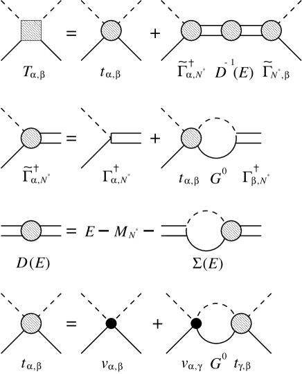
FIG. 2.: Graphical representation of the scattering equations defined by Eqs. (65) -(71).

FIG. 3.: Mass splitting $\delta^{*}$(Eq.(70)) of $N^{*}$ as a function of the matrix element $\alpha$(Eq.(71) of the tensor potential. Both are in units of $\Delta$-$N$ mass difference $\delta$.

FIG. 4.: Mixing coefficient of the $N^{*}$ eigenfunctions (Eqs.(72)-(73)) as a function of the matrix element $\alpha$(Eq.(71)) of the tensor potential.

FIG. 5.: $N^{*}\rightarrow\eta N$ strength as a function of the matrix element $\alpha$(Eq.(71)) of the tensor potential. The solid and dashed curves are the strengths for $N^{*}_{L}$ and $N^{*}_{H}$, respectively.

FIG. 6.: Same as Fig. 5 except for the $\pi N$ transition.

FIG. 7.: Mass of $\Delta$ as a function of the cutoff $\Lambda_{\rm g}$ in the OGE model. The solid, dashed and dot-dashed curves are results with $\alpha_{s}=0.8,1.0$ and $1.6$, respectively. Here the nucleon mass is normalized to $940$ MeV and $\alpha_{c}=4$ fm^-2 is used.

FIG. 8.: Mass of $N^{*}_{L}$ as a function of $\alpha_{s}$ in the OGE model. The solid, dashed and dot-dashed curves are results with $\alpha_{c}=3,4$ and $5$ fm^-2. For each value of $\alpha_{c}$ and $\alpha_{s}$, the cutoff parameter $\Lambda_{\rm g}$ is determined by requiring the mass of $\Delta$ to be $1300$ MeV.

FIG. 9.: Mass splitting of $N^{*}$’s in the OGE model. See caption of Fig. 8.

FIG. 10.: Mass of $\Delta$ as a function of $\Lambda_{\pi}$ in the OME model. The solid, dashed and dot-dashed curves are the results with $\alpha_{c}=2,3$ and $4$ fm^-2 and $\Lambda_{\eta}=1$ GeV.

FIG. 11.: Mass of $N^{*}_{L}$ as a function of $\alpha_{c}$ in the OME model. The cutoff $\Lambda_{\pi}$ for each $\alpha_{c}$ is determined so that the mass of $\Delta$ is $1300$ MeV.

FIG. 12.: Mass splitting of $N^{*}$ in the OME model. See caption of Fig. 11.

(a)

(b)

FIG. 13.: $\Delta\rightarrow\pi N$ vertex function in the OGE model (a) and the OME model (b). The solid and dashed curves are the vertex functions with and without the quark form factor $F(k)$, respectively. The dot-dashed curve is the vertex function of the SL model.

FIG. 14.: Phase shifts of the $\pi N$ scattering in $S_{11}$ channel. The solid and dashed curves are the results from the OGE and OME models, respectively. Open circles are the data of VPI SP98 [25].

(a)

(b)

FIG. 15.: Same as Fig. 14 except for the real parts (a) and the imaginary parts (b) of the $\pi N$ scattering amplitudes in $S_{11}$ channel.

(a)

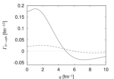
(b)

FIG. 16.: $N^{*}\rightarrow\pi N$ vertex functions calculated from the OGE model (a) and the OME model (b). The solid and dashed curves are for $N^{*}_{L}$ and $N^{*}_{H}$, respectively.

(a)

(b)

FIG. 17.: Same as Fig. 16 except for the $N^{*}\rightarrow\eta N$ vertex functions.

(a)

(b)

FIG. 18.: Same as Fig. 16 except for the $N^{*}\rightarrow\pi\Delta$ vertex functions.

(a)

(b)

FIG. 19.: Real parts of the eigenvalues of $D(E)$(Eq.(63)) calculated from the OGE model (a) and the OME model (b). The solid and dashed curves correspond to the masses for $N^{*}_{L}$ and $N^{*}_{H}$, respectively. The dotted line represents Re$(E^{*})=W_{\rm cm}$.

(a)

(b)

FIG. 20.: Same as Fig. 19 except for the imaginary parts of the eigenvalues of $D(E)$.

(a)

(b)

(c)

FIG. 21.: $N^{*}\rightarrow\pi N$ (a), $N^{*}\rightarrow\eta N$ (b), and $N^{*}\rightarrow\pi\Delta$ (c) vertex functions in the phenomenological model. The solid and dashed curves are for $N^{*}_{L}$ and $N^{*}_{H}$, respectively.

FIG. 22.: Phase shifts of the $\pi N$ scattering in $S_{11}$ channel calculated from the phenomenological model. Open circles are data from VPI SP98

(a)

(b)

FIG. 23.: Same as Fig. 22 except for the real parts (a) and imaginary parts (b) of the $\pi N$ scattering amplitudes of in $S_{11}$.

(a)

(b)

FIG. 24.: Real parts (a) and imaginary parts (b) of the eigenvalues of $D(E)$(Eq.(63)) calculated from the phenomenological model. The solid and dashed curves correspond to the masses for $N^{*}_{L}$ and $N^{*}_{H}$, respectively.

FIG. 25.: Total cross section of $\pi^{-}+p\rightarrow\eta+n$ reaction. The dashed, dot-dashed and solid curves are results of the OME, OGE and phenomenological models. Data are taken from Ref. [36].