Continued fraction representation of the Coulomb Green’s operator
and unified description of bound, resonant and scattering states

Abstract

If a quantum mechanical Hamiltonian has an infinite symmetric tridiagonal (Jacobi) matrix form in some discrete Hilbert-space basis representation, then its Green’s operator can be constructed in terms of a continued fraction. As an illustrative example we discuss the Coulomb Green’s operator in Coulomb–Sturmian basis representation. Based on this representation, a quantum mechanical approximation method for solving Lippmann–Schwinger integral equations can be established, which is equally applicable for bound-, resonant- and scattering-state problems with free and Coulombic asymptotics as well. The performance of this technique is illustrated with a detailed investigation of a nuclear potential describing the interaction of two $\alpha$ particles.

]

I Introduction

Green’s operators play a central role in theoretical physics, especially in quantum mechanics, as they appear in fundamental equations governing the dynamics of physical systems. The formalisms based on Green’s operators represent alternative, but essentially equivalent way of describing the same systems as methods based on differential equations. However, since Green’s operators are related to the integral equation formalism, their use is more advantageous in many cases than that of traditional differential approaches: boundary conditions, for example, are automatically incorporated in the formalism. Although the concept of Green’s operators frequently appears in basic textbooks on the level of fundamental equations, in practical calculations their use is usually avoided, and various approximations to the Schrödinger equation are preferred instead. The reason certainly is that the evaluation of Green’s operators is much more complicated than the direct treatment of the Hamiltonian using standard tools of theoretical and mathematical physics.

The discrete Hilbert-space basis representation of the Green’s operator is very advantageous since it makes the solution of the Lippmann–Schwinger-type integral equations possible on an easy-to-apply, yet very general way. If the integral equation possesses good mathematical properties, then the potential term can be well approximated on a finite subset of the Hilbert-space basis and the integral equation can be solved without any further approximation. This concept has already been elaborated in several different forms. In Refs. [1, 2] harmonic oscillator functions were used, which allowed the representation of the free Green’s operator, and thus the corresponding approximation method can handle problems with free asymptotics. In Refs. [3, 4, 5, 6] Coulomb–Sturmian basis was applied, which allowed the inclusion of the long-range Coulomb potential into the Green’s operator, and thus led to the exact treatment of the Coulomb asymptotics. This latter approach has also been extended to solving the three-body Coulomb problem in the Faddeev approach. So far good results have been reached for bound-state [7] and below-breakup scattering-state problems [8]. These results have showed the efficiency of the discrete Hilbert-space expansion method in solving fundamental integral equations. We note that in all the previous approaches [3, 4, 5, 6, 7, 8] the Coulomb Green’s matrix has been determined in a rather complicated way with the aid of special functions.

In Ref. [9] we have presented a rather general and easy-to-apply method for calculating the discrete Hilbert-space basis representation of the Green’s operators of those Hamiltonians, which have infinite symmetric tridiagonal (i.e. Jacobi) matrix forms. The procedure necessitates the evaluation of the Hamiltonian matrix on this basis, a rather common task in quantum mechanics. Then the elements of the Jacobi matrix are used as input in the calculation of the Green’s matrix in terms of a continued fraction. This way of calculating Green’s matrices simplifies the calculations considerably and the representation via continued fraction provides a readily computable way. The combination of this new way of calculating the Coulomb Green’s matrix with the technique of solving integral equations in discrete Hilbert–space-basis representation results a quantum mechanical approximation method which is rather general in the sense that it is equally applicable to solving bound-, resonant- and scattering-state problems with practically any potential of physical relevance. And all this is provided at a very little cost: in practice only matrix elements of the Hamiltonian are required.

The structure of this paper is the following. In section II we consider the Coulomb Green’s operator in Coulomb–Sturmian representation. We show that this Coulomb Green’s matrix can be given in terms of a continued fraction. In section III the solution method of the Lippmann–Schwinger equation in Coulomb-Sturmian space representation is explained, and the method is applied to describe bound, resonance and scattering solutions of a model nuclear potential. Finally conclusions are drawn in section IV.

II Continued fraction representation of the Coulomb Green’s operator

Let us consider the radial Coulomb Hamiltonian

$$H^{\rm C}_{l}=-\frac{\hbar^{2}}{2m}\left(\frac{\mbox{d}^{2}}{\mbox{d}r^{2}}+\frac{l(l+1)}{r^{2}}\right)+\frac{Z{\rm e}^{2}}{r}\ ,$$ (1)

where $m$, $l$, ${\rm e}$ and $Z$ stand for the mass, angular momentum, electron charge and charge number, respectively. The Coulomb–Sturmian (CS) functions, the Sturm–Liouville solutions of the Hamiltonian (1) [12], appear as

$$\langle r|n\rangle=\sqrt{\frac{n!}{(n+2l+1)!}}\ \exp(-br)(2br)^{l+1}L_{n}^{(2l+1)}(2br)\ ,$$ (2)

where $b$ is a scale parameter, $n$ is the radial quantum number and $L_{n}^{(\alpha)}$ denotes the generalized Laguerre polynomials [13]. With the biorthonormal partner defined by $\langle r|\widetilde{n}\rangle\equiv\langle r|n\rangle/r$ these functions form a discrete basis. We denote the Coulomb Green’s operator as $G^{\rm C}_{l}(z)=(z-H^{\rm C}_{l})^{-1}$ and we consider here its CS matrix elements $\underline{G}^{\rm C}_{nn^{\prime}}=\langle\widetilde{n}|G^{\rm C}_{l}|\widetilde{n^{\prime}}\rangle$.

The starting point in this procedure is the observation the the matrix $\underline{J}^{\rm C}_{nn^{\prime}}=\langle n|(z-H^{\rm C}_{l})|n^{\prime}\rangle$ possesses an infinite symmetric tridiagonal i.e. Jacobi structure,

$$\underline{J}^{\rm C}_{nn}=2(n+l+1)(k^{2}-b^{2})\frac{\hbar^{2}}{4mb}-Z{\rm e}^{2}$$ (3)

and

$$\underline{J}^{\rm C}_{nn-1}=-[n(n+2l+1)]^{1/2}(k^{2}+b^{2})\frac{\hbar^{2}}{4mb}\ ,$$ (4)

where $k=(2mz/\hbar^{2})^{1/2}$ is the wave number. The main result of Ref. [9] is that for Jacobi matrix systems the $N$’th leading submatrix $\underline{G}^{{\rm C}(N)}_{ij}$ of the infinite Green’s matrix can be determined by the elements of the Jacobi matrix

$$\underline{G}^{{\rm C}(N)}_{ij}=[\underline{J}^{\rm C}_{ij}+\delta_{jN}\,\,\delta_{iN}\,\,\underline{J}^{\rm C}_{NN+1}\,\,C]^{-1}\ ,$$ (5)

where $C$ is a continued fraction

$$C=-\frac{u_{N}}{d_{N}+\frac{\displaystyle u_{N+1}}{\displaystyle d_{N+1}+\frac{\displaystyle u_{N+2}}{\displaystyle d_{N+2}+\cdots}}}\ ,$$ (6)

with coefficients

$$u_{i}=-{\underline{J}^{\rm C}_{i,i-1}}/{\underline{J}^{\rm C}_{i,i+1}},\quad d_{i}=-{\underline{J}^{\rm C}_{i,i}}/{\underline{J}^{\rm C}_{i,i+1}}\ .$$ (7)

In Ref. [9] we have shown that the continued fraction $C$, as it stands, is convergent only for negative energies, but it can be continued analytically to the whole complex energy plane. Since the $u_{i}$ and $d_{i}$ coefficients possess the limit properties

$$u\equiv\lim_{i\rightarrow\infty}u_{i}=-1$$ (8)

and

$$d\equiv\lim_{i\rightarrow\infty}d_{i}=2(k^{2}-b^{2})/(k^{2}+b^{2})\ ,$$ (9)

the continued fraction appears as

$$C=-\frac{u_{N}}{d_{N}+\frac{\displaystyle u_{N+1}}{\displaystyle d_{N+1}+\cdots+\frac{\displaystyle u}{\displaystyle d+\frac{\displaystyle u}{\displaystyle d+\cdots}}}}\ .$$ (10)

The tail $w$ of $C$ satisfies the implicit relation

$$w=\frac{u}{d+w}\ ,$$ (11)

which is solved by

$$w_{\pm}=(b\pm{\mathrm{i}}k)^{2}/(b^{2}+k^{2})\ .$$ (12)

Replacing the tail of the continued fraction by its explicit analytical form $w_{\pm}$, we can speed up the convergence and, which is more important, turn a non-convergent continued fraction into a convergent one [11]. In fact, by using $w_{\pm}$ instead of the non-converging tail we perform an analytic continuation. In Ref. [9] we have shown that $w_{+}$ provides an analytic continuation of the Green’s matrix to the physical, while $w_{-}$ to the unphysical Riemann-sheet. This way Eq. (6) together with (5) provide the CS basis representation of the Coulomb Green’s operator on the whole complex energy plane. We note here that with the choice of $Z=0$ the Coulomb Hamiltonian (1) reduces to the kinetic energy operator and our formulas provide the CS basis representation of the Green’s operator of the free particle as well.

We can immediately test $\underline{G}^{C}$ by calculating eigenvalues belonging to attractive Coulomb interactions. Fig. 1 shows $|{\underline{G}^{C}}(E)|$. The poles coincide with the exact Coulomb energy levels up to machine accuracy. We stress that, from the point of view of determining the energy eigenvalues, the rank $N$ of the matrix and the specific choice of the CS basis parameter are irrelevant. Any representation of the Coulomb Green’s operator exhibits all the properties of the system and our Green’s matrix contains all the infinitely many eigenvalues. This is especially interesting if we compare with the usual procedure of calculating eigenvalues of a finite Hamiltonian matrix which could only provide an upper limit for the N lowest eigenvalues. Our procedure does not truncate the Coulomb Hamiltonian, because all the higher $\underline{J}_{nn^{\prime}}$ matrix elements are implicitly contained in the continued fraction. We note that $\underline{G}^{C}$ has already been calculated before [3, 4, 5, 6] by using $\mbox{}_{2}F_{1}$ hypergeometric functions [13]. In Ref. [9] we have shown that the two formalism lead to numerically identical results for all energies and the continued fraction representation possesses all the analytic properties of $G^{C}$ also in practice.

III Solution of the Lippmann-Schwinger integral equation in CS representation

In this section, after Refs. [3, 4, 5, 6], we recapitulate the solution of the Lippmann–Schwinger equation in CS representation. We suppose that the Hamiltonian $H_{l}$ is split into two terms

$$H_{l}=H_{l}^{\rm C}+V_{l}\ ,$$ (13)

where $V_{l}$ is the asymptotically irrelevant short-range potential. The Green’s operator of $H_{l}$ is defined by $G_{l}(z)=(z-H_{l})^{-1}$, and it is connected to $G_{l}^{\rm C}(z)$ via the resolvent relation

$$G_{l}(z)=G_{l}^{\rm C}(z)+G_{l}^{\rm C}(z)V_{l}G_{l}(z)\ .$$ (14)

The wave function $|\Psi^{(\pm)}_{l}\rangle$ describing a scattering process satisfies the inhomogeneous Lippmann–Schwinger equation [14]

$$|\Psi^{(\pm)}_{l}\rangle=|\Phi^{(\pm)}_{l}\rangle+G_{l}^{\rm C}(E\pm{\rm i}0)V_{l}|\Psi^{(\pm)}_{l}\rangle\ ,$$ (15)

where $|\Phi^{(\pm)}_{l}\rangle$ is the solution of the Hamiltonian $H^{\rm C}_{l}$ possessing scattering asymptotics. The bound- and resonant-state wave functions satisfy the homogeneous Lippmann–Schwinger equation

$$|\Psi_{l}\rangle=G_{l}^{\rm C}(E)V_{l}|\Psi_{l}\rangle$$ (16)

at real negative and complex $E$ energies, respectively.

We are going to solve these equations in a unified way by approximating only the potential term $V_{l}$. For this purpose we write the unit operator in the form

$${\bf 1_{l}}=\lim_{N\to\infty}{\bf{1}}_{lN}\ ,$$ (17)

where

$${\bf{1}}_{lN}=\sum_{n=0}^{N}|\tilde{n}\rangle\sigma_{n}^{N}\langle n|=\sum_{n=0}^{N}|n\rangle\sigma_{n}^{N}\langle\tilde{n}|\ .$$ (18)

The $\sigma$ factors have the properties $\lim_{n\to\infty}\sigma_{n}^{N}=0$ and $\lim_{N\to\infty}\sigma_{n}^{N}=1$, and make the limit in (17) smoother. They were introduced originally for improving the convergence properties of truncated trigonometric series [15], but they turned out to be also very efficient in solving integral equations in discrete Hilbert space basis representation [16]. The choice of $\sigma_{n}^{N}$

$$\sigma_{n}^{N}=\frac{1-\exp\{-[\alpha(n-N-1)/(N+1)]^{2}\}}{1-\exp(-\alpha^{2})}$$ (19)

with $\alpha\sim 5$ has proved to be appropriate in practical calculations.

Let us introduce an approximation of the potential operator

$$V_{l}={\bf 1_{l}}V_{l}{\bf 1_{l}}\approx{\bf{1}}_{lN}V_{l}{\bf{1}}_{lN}=V_{l}^{N}=\sum_{n,n^{\prime}=0}^{N}|\widetilde{n}\rangle\;\underline{V}_{nn^{\prime}}\;\mbox{}\langle\widetilde{n^{\prime}}|\ ,$$ (20)

where the matrix elements

$$\underline{V}_{nn^{\prime}}=\sigma^{N}_{n}\langle n|V_{l}|n^{\prime}\rangle\sigma^{N}_{n^{\prime}}\ ,$$ (21)

in general, have to be calculated numerically. This approximation is called separable expansion, because the operator $V_{l}^{N}$, e.g. in coordinate representation, appears in the form

$$\langle r|V^{N}|r^{\prime}\rangle=\sum_{n,n^{\prime}=0}^{N}\langle r|\widetilde{n}\rangle\;\underline{V}_{nn^{\prime}}\;\mbox{}\langle\widetilde{n^{\prime}}|r^{\prime}\rangle\ ,$$ (22)

i.e.  the dependence on $r$ and $r^{\prime}$ appears in a separated functional form.

With this separable potential Eqs. (15) and (16) reduce to

$$|\Psi^{(\pm)}_{l}\rangle=|\Phi^{(\pm)}_{l}\rangle+\sum_{n,n^{\prime}=0}^{N}G^{\rm C}_{l}(E\pm{\rm i}0)|\widetilde{n}\rangle\;\underline{V}_{nn^{\prime}}\;\mbox{}\langle\widetilde{n^{\prime}}|\Psi^{(\pm)}_{l}\rangle\ ,$$ (23)

and

$$|\Psi_{l}\rangle=\sum_{n,n^{\prime}=0}^{N}G_{l}^{\rm C}(E)|\widetilde{n}\rangle\;\underline{V}_{nn^{\prime}}\;\mbox{}\langle\widetilde{n^{\prime}}|\Psi_{l}\rangle\ ,$$ (24)

respectively. To derive equations for the coefficients $\underline{\Psi}_{l}^{(\pm)}=\langle\widetilde{n^{\prime}}|\Psi_{l}^{(\pm)}\rangle$ and $\underline{\Psi}_{l}=\langle\widetilde{n^{\prime}}|\Psi_{l}\rangle$, we have to act with states $\langle\widetilde{n^{\prime\prime}}|$ from the left. Then the following inhomogeneous and homogeneous algebraic equations are obtained, for scattering and bound-state problems, respectively:

$$[(\underline{G}^{\rm C}_{l}(E\pm{\rm i}0))^{-1}-\underline{V}_{l}]\underline{\Psi}_{l}^{(\pm)}=\underline{\Phi}_{l}^{(\pm)},$$ (25)

and

$$[(\underline{G}_{l}^{\rm C}(E))^{-1}-\underline{V}_{l}]\underline{\Psi}_{l}=0\ ,$$ (26)

where the overlap ${\Phi}_{nl}^{(\pm)}=\langle\widetilde{n}|\Phi_{l}^{(\pm)}\rangle$ can also be calculated analytically [4]. The homogeneous equation (26) is solvable if and only if

$$\det[(\underline{G}_{l}^{\rm C}(E))^{-1}-\underline{V}_{l}]=0$$ (27)

holds, which is an implicit nonlinear equation for the bound- and resonant-state energies. As far as the scattering states concerned the solution of (25) provides the overlap $\langle\widetilde{n}|\Psi_{l}\rangle$. From this quantity any scattering information can be inferred, for example the scattering amplitude corresponding to potential $V_{l}$ is given by [14]

$$A^{V}=\langle\Phi^{(-)}_{l}|V_{l}|\Psi^{(+)}_{l}\rangle=\underline{\Phi}_{l}^{(-)}\underline{V}_{l}\;\underline{\Psi}_{l}^{(+)}.$$ (28)

Note that also the Green’s matrix of the total Hamiltonian, which is equivalent to the complete solution of the physical system, can be constructed as the solution of Eq. (14)

$$\underline{G}_{l}(z)=[(\underline{G}_{l}^{\rm C}(z))^{-1}-\underline{V}_{l}]^{-1}\ .$$ (29)

Finally, it should also be emphasized, that in this approach only the potential operator is approximated, but the asymptotically important $H^{\rm C}$ term remains intact. The solutions are defined on the whole Hilbert space, not only on a finite subspace. The wave functions are not linear combinations of basis functions, but rather, as Eqs. (23) and (24) indicate, linear combinations of the states $G_{l}^{\rm C}(E)|\widetilde{n}\rangle$, which have been shown to possess correct Coulomb asymptotics [5].

A Bound, resonant and scattering states in a model nuclear potential

In this subsection we apply the above techniques to calculate bound-, resonant- and scattering-state solutions of potential problems. The particular example we consider is a potential representing the interaction of two $\alpha$ particles. This example is thoroughly discussed in the pedagogical work [17] in the context of a conventional approach based on the numerical solution of the Schrödinger equation. The interaction of two $\alpha$ particles can be approximated by the potential

$${V}_{\alpha-\alpha}(r)=-A\exp(-\beta r^{2})+\frac{Z^{2}{\rm e}^{2}}{r}\ {\rm erf}(\gamma r),$$ (30)

where ${\rm erf}(z)$ is the error function [13]. This potential is a composition of a bell-shaped deep, attractive nuclear potential, and a repulsive electrostatic field between two extended charged objects. The units used in the Hamiltonian of this system are suited to nuclear physical applications, i.e. the energy and length scale are measured in MeV and fm, respectively. In these units $\hbar/(2m)=10.375$ MeV fm² (with $m$ being the reduced mass of two $\alpha$ particles) and ${\rm e}^{2}=1.44$ MeV fm. The other parameters are $A=$122.694 MeV, $\beta=0.22$ fm^-2, $\gamma=0.75$ fm^-1 and $Z=2$ (the charge number of the $\alpha$ particles).

Since the $\alpha-\alpha$ potential possesses a Coulomb tail, for the asymptotically relevant operator we should take the Coulomb Hamiltonian $H^{\rm C}$ of Eq. (1) and the short-range potential is then defined by

$$V(r)=V_{\alpha-\alpha}(r)-\frac{Z^{2}{\rm e}^{2}}{r}=-A\exp(-\beta r^{2})-\frac{Z^{2}{\rm e}^{2}}{r}\ {\rm erfc}(\gamma r),$$ (31)

with ${\rm erfc}(z)=1-{\rm erf}(z)$. We approximate the short-range potential $V(r)$ according to Eq. (20) on the CS basis. From this point on, however, the properties of the physical system will be buried into the numerical values of the matrix elements. Thus the method is applicable to all types of potentials, as long as we can calculate their matrix elements somehow. Besides ordinary potentials this equally applies to complex, momentum-dependent, non-local, etc.  potentials relevant to practical problems of atomic, nuclear and particle physics. Furthermore, the present formalism is equally suited to problems including attractive or repulsive long-range Coulomb-like and short-range potentials.

It should also be emphasized again that in this approach only the potential operator $V$ is approximated and the resulting wave function possesses the correct asymptotics. So, if the parameter $b$ is chosen such that $V^{N}$ in (20) approaches $V$ uniformly, the convergence of the bound-, resonant- and scattering-state quantities with respect to increasing $N$ will also be uniform, thus $V^{N}$ provides more or less uniformly good approximation to $V$ on the whole spectrum of physical interest.

1 Bound states

First we consider only the nuclear part of potential (30) and switch off the Coulomb interaction by setting $Z=0$. According to Ref. [17], this potential supports altogether four bound states: three with $l=0$ and one with $l=2$. However, it is known that the first two $l=0$ and the single $l=2$ state are unphysical, because they are forbidden due to the Pauli principle. This fact is not taken into account in this simple potential model. Although from the physical point of view these Pauli-forbidden states have to be dismissed as unphysical, they are legitimate solutions of our simple model potential. The proper inclusion of the Pauli principle in the model would turn the potential into a non-local one. This problem has been considered within the present method in Ref. [4].

As illustrative examples we present the results of our calculations for the three $l=0$ states. We determined the energies of these states from Eq. (27), using the CS parameter $b=4$ fm^-1. Table I shows the convergence of the method with respect to $N$, the number of basis states used in the expansion. It can be seen that the method is very accurate, convergence up to 12 digits can easily been reached. We note that according to Ref. [17], the energy of the two lowest (i.e. the unphysical) $l=0$ states is $E=-76.903\ 6145$ and $-29.000\ 48$ MeV in the uncharged case, which is in reasonable agreement with our results.

2 Resonance states

Switching on the repulsive Coulomb interaction ($Z=2$) the bound states are shifted to higher energies. The most spectacular effect is that the third $l=0$ state, which is located at $E=-1.608\ 740\ 8214$ MeV in the uncharged case, moves to positive energies and becomes a resonant state. This is in agreement with the observations: the $\alpha-\alpha$ system (i.e. the ⁸Be nucleus) does not have a stable ground state, rather it decays with a half life of $7\times 10^{-17}$ sec.

In our calculations we determined the energy corresponding to this resonance and to other ones as well by the same techniques we used before to find bound states. In fact, we used the same computer code and the same CS parameter ($b=4$ fm^-1) as we used in the analysis of bound states. The method, again, requires locating the poles of the Green’s matrix, but not on the real energy axis, rather on the complex energy plane. In Table II we demonstrate the convergence of our method with respect to $N$ for the lowest $l=0$ and $l=2$ resonance states. In Fig. 2 we plotted the modulus of the determinant of the Green’s matrix (as in Eq. (29)) $|\underline{G}(E)|$ over the complex energy plane for $l=2$. The resonance is located at the pole of this function. Finally, we mention that there is a resonance state for $l=4$ at $E=11.791\ 038-{\rm i\ }1.788\ 957$ MeV.

Although it is not our aim here to reproduce experimental data with this simple potential model, we note that the corresponding experimental values [18] are $E_{{\rm r},l=0}=$0.09189 MeV, $E_{{\rm r},l=2}=$3.132 $\pm$ $0.030$ MeV, $E_{{\rm r},l=4}=$11.5 $\pm$ 0.3 MeV, and $\Gamma_{l=0}/2=(3.4\pm 0.9)\times 10^{-6}$ MeV, $\Gamma_{l=2}/2$=0.750 $\pm$ 0.010 MeV, $\Gamma_{l=4}/2\simeq$1.75 MeV.

3 Scattering states

In order to demonstrate the performance of our approach for scattering states we calculated scattering phase shifts $\delta_{l}(E)$ for ${V}_{\alpha-\alpha}(r)$ in (30). As described previously in this section, phase shifts can be extracted from the scattering amplitude given in Eq. (28). Specifying this formula for the Coulomb-like case and for a given partial wave $l$ we have

$$a_{l}=\frac{1}{k}\exp({\rm i}(2\eta_{l}+\delta_{l}))\sin\delta_{l}\ ,$$ (32)

where $a_{l}$ is the Coulomb-modified scattering amplitude corresponding to the short-range potential, $\eta_{l}={\rm arg}\Gamma(l+i\gamma+1))$ is the phase shift of the Coulomb scattering with $\gamma=Z^{2}{\rm e}^{2}m/\hbar^{2}k$ and $\delta_{l}$ is the phase shift due to the short-range potential.

The convergence of the method with respect to $N$ is demonstrated in Table III, where $\delta_{0}(E)$ is displayed at three different energy values $E$. As in our calculations for the bound and the resonance states, we used $b=4$ fm^-1here too.

In Fig. 3 we plotted the scattering phase shifts $\delta_{l}(E)$ for $l=0$, 2 and 4 up to $E=30$ MeV. In all three plots in Fig. 3 the location of the corresponding resonance is clearly visible as a sharp rise of the phase around the resonance energy $E_{\rm r}$. This rise is expected to be more sudden for sharp resonances, and this is, in fact, the case here too. The phase changes with an abrupt jump of $\pi$ for the sharp $l=0$ resonance, while it is slower for the broader $l=2$ and $l=4$ resonances. We also note that the phase shifts plotted in Fig. 3 are also in accordance with the Levinson theorem, which states that $\delta_{l}(0)=m\pi$, where $m$ is the number of bound states in the particular angular momentum channel. Indeed, as we have discussed earlier, there are two bound states for $l=0$, one for $l=2$ and none for $l=4$.

As an illustration of the importance of the smoothing factors we show in Fig. 4 the convergence of the phase shift $\delta_{0}(E)$ at a specific energy $E=10$ MeV with and without the smoothing factors $\sigma_{n}^{N}$ in (18), and consequently in (21). (Here and everywhere else the $\alpha$ parameter was chosen to be 5.2.) Clearly, the convergence is much poorer without the smoothing factors. We note that this also applies to the other quantities calculated for bound and resonance states.

Finally, we should call the attention upon the fact that this method is very accurate. Reasonable accuracy is reached already at relatively small basis, around $N=20$. The accuracy gained in larger bases is beyond most of the practical requirements. Test calculations have been performed on a linux PC (Intel PII, 266 MHz) using double precision arithmetic. The calculation of a typical bound- or resonant-state energy requires the evaluation of the potential matrix by Gauss-Laguerre quadrature and finding the zeros of the determinant (27), which incorporates the evaluation of the Coulomb Green’s matrix and the the calculation of a determinant by performing an LU decomposition in each steps. The determination of the energy value in the first column and last row of Table I, which meant $6$ steps in the zero search and handling of $40\times 40$ matrices, took $0.06$ sec. The corresponding resonance energy value in Table II required $12$ steps in the zero search on the complex energy plane and $0.8$ sec. The evaluation of the three phase shift values in the last row of Table III took $0.19$ sec., $0.11$ sec. and $0.08$ sec., respectively. So, this method is not only extremely accurate but also very fast.

IV Conclusions

In this work we have presented a continued fraction representation of the Coulomb Green’s operator on Coulomb–Sturmian basis. Numerical illustrations show that this representations is simple, readily computable and numerically exact on the whole complex energy plane. This result is based on the observation that in this basis the Coulomb Hamiltonian possesses a Jacobi matrix structure. These techniques can be transferred to other problems, where the Hamiltonian matrix also has a Jacobi form. Examples for this are the harmonic oscillator [9], the generalized Coulomb problem [19], which contains both the $D$ dimensional harmonic oscillator and the Coulomb problems as special limits and the relativistic Coulomb problem [20].

Once the representation of the Coulomb Green’s operator in the discrete CS basis is available, we can proceed to solve the Lippmann–Schwinger integral equation. In practice this means the approximation of the potential term on a finite subset of this basis. This is the only stage where approximations are made, otherwise this method is exact and analytic, and provides asymptotically correct solutions. Consequently, bound, resonance and scattering problems can be treated on an equal footing, while these phenomena are usually discussed in rather different ways in conventional quantum mechanical approaches. This unified treatment is also reflected by the fact that all the calculations are made using the same discrete basis, containing also the same basis and other parameters. Furthermore, this approach is applicable to a wide range of potential problems, including complex, momentum-dependent, non-local, etc. ones. These techniques were illustrated with calculations for a model nuclear potential describing the interaction of two $\alpha$ particles.

Once a discrete Hilbert-space basis representation of the Green’s operator of the free or Coulomb Hamiltonian is at our disposal, we can also construct the matrix representation of the Green’s operator of the total Hamiltonian by solving a resolvent equation. This provides a complete description of the two-body system. The Green’s operators, similarly to the wave functions, contain all the information about the system, and any physical property can be derived from them. The importance of this result is not purely formal, but it provides us with an effective tool in practical calculations for realistic physical problems. Moreover, from the Green’s matrices of simpler systems, the Green’s matrices of more complex composite systems can be constructed. These techniques have been used so far for solving Faddeev equations of some three-body Coulombic systems [7, 8] but they can certainly be adapted to other challenging problems as well.

TABLE I.: Convergence of the $l=0$ bound-state energy eigenvalues $E_{nl}$ in $V_{\alpha-\alpha}(r)$ in the uncharged ($Z=0$) case. $N$ denotes the number of basis states used in the expansion.

$N$	$E_{00}$ (MeV)	$E_{10}$ (MeV)	$E_{20}$ (MeV)
8	$-$76.903 557 1529	$-$29.005 234 9134	$-$1.739 478 2626
10	$-$76.903 609 9717	$-$29.000 352 3141	$-$1.637 269 0831
15	$-$76.903 614 3090	$-$29.000 469 8249	$-$1.608 824 6403
18	$-$76.903 614 3254	$-$29.000 470 2338	$-$1.608 742 5166
20	$-$76.903 614 3263	$-$29.000 470 2566	$-$1.608 741 0685
25	$-$76.903 614 3265	$-$29.000 470 2623	$-$1.608 740 8256
28	$-$76.903 614 3265	$-$29.000 470 2625	$-$1.608 740 8216
30	$-$76.903 614 3265	$-$29.000 470 2625	$-$1.608 740 8213
35	$-$76.903 614 3265	$-$29.000 470 2626	$-$1.608 740 8214
40	$-$76.903 614 3265	$-$29.000 470 2626	$-$1.608 740 8214

TABLE II.: Convergence of the energy eigenvalues $E_{{\rm res},l}$ for the $l=0$ and $l=2$ resonances in the $V_{\alpha-\alpha}(r)$ potential. $N$ denotes the number of basis states used in the expansion.

$N$	$E_{{\rm res},0}$ (MeV)	$E_{{\rm res},2}$ (MeV)
8	$-$0.000 854 9596 $+$i 0.000 000 0000	2.807 21 $-$i 0.607 11
10	$-$0.063 364 2503 $-$i 0.000 000 0681	2.866 30 $-$i 0.628 56
15	$-$0.091 785 0787 $-$i 0.000 002 8092	2.889 68 $-$i 0.620 99
18	$-$0.091 963 0277 $-$i 0.000 002 8572	2.889 34 $-$i 0.620 53
20	$-$0.091 969 7296 $-$i 0.000 002 8588	2.889 24 $-$i 0.620 56
25	$-$0.091 971 8479 $-$i 0.000 002 8592	2.889 23 $-$i 0.620 62
28	$-$0.091 971 9788 $-$i 0.000 002 8592	2.889 25 $-$i 0.620 62
30	$-$0.091 972 0064 $-$i 0.000 002 8592	2.889 25 $-$i 0.620 61
35	$-$0.091 972 0258 $-$i 0.000 002 8592	2.889 24 $-$i 0.620 61
40	$-$0.091 972 0290 $-$i 0.000 002 8592	2.889 25 $-$i 0.620 61

TABLE III.: Convergence of the $\delta_{0}(E)$ phase shift (in radians) in the $V_{\alpha-\alpha}(r)$ potential at three different energies. $N$ denotes the number of basis states used in the expansion.

$N$	$E=0.1$ MeV	$E=1$ MeV	$E=30$ MeV
8	6.283 230	8.817 731	7.783 217
10	9.424 059	8.862 581	4.817 163
15	9.424 018	8.859 651	4.835 479
18	9.424 022	8.859 467	4.829 861
20	9.424 023	8.859 441	4.828 882
25	9.424 024	8.859 419	4.828 563
28	9.424 024	8.859 414	4.828 555
30	9.424 024	8.859 412	4.828 554
35	9.424 024	8.859 411	4.828 552
40	9.424 024	8.859 411	4.828 552

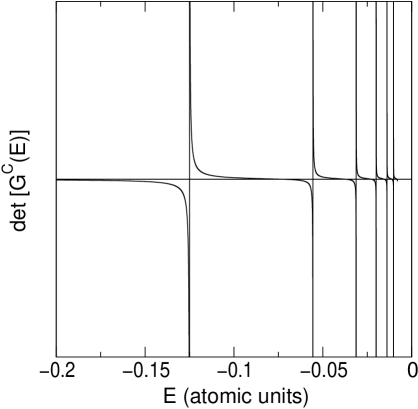
FIG. 1.: The determinant of a $3\times 3$ Coulomb Green’s matrix ${\rm det}[\underline{G}^{C}(E)]$ as the function of the energy $E$ for $l=1$. The bound states of the Coulomb problem are located at energies where the vertical lines cross the horizontal axis. (These lines are shown only for demonstrative purposes: they do not correspond to functional values of ${\rm det}[\underline{G}^{C}(E)]$.) Atomic units of $m={\rm e}=\hbar=1$ and $Z=-1$ were used. For the sake of clarity only the first 6 energy levels are shown. These are located at $E_{n}=-1/[2(n+l+1)]^{2}$ with $n\leq 5$.

FIG. 2.: The modulus of the determinant of the $\underline{G}(E)$ Green’s matrix for the $\alpha-\alpha$ potential on the complex energy plane for $l=2$. The pole at $E=2.889\ 25-{\rm i\ }0.620\ 61$ MeV corresponds to a resonance.

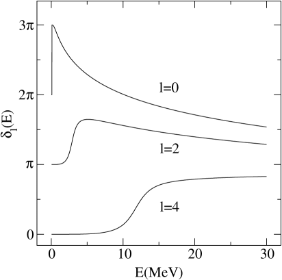
FIG. 3.: Scattering phase shifts $\delta_{l}(E)$ (in radians) in the $\alpha-\alpha$ potential for $l=0$, 2 and 4. The resonances in these partial waves appear as sharp rises in the corresponding phase shifts. In these calculations a basis with $N=35$ was used.

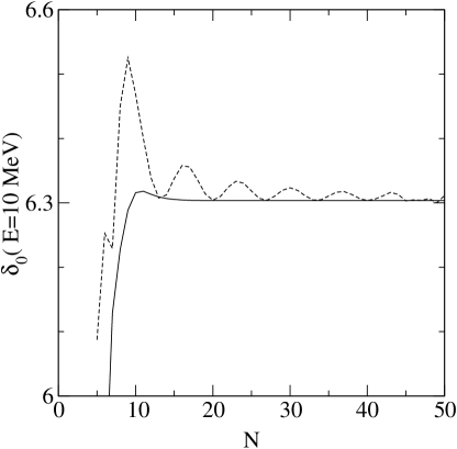
FIG. 4.: Convergence of the scattering phase shift $\delta_{0}(E)$ (in radians) at $E=10$ MeV calculated with (solid line) and without (dashed line) smoothing factors.

REFERENCES

- [1] J. Révai, JINR Preprint E4-9429, Dubna, 1975.
- [2] F. A. Gareev, M. Ch. Gizzatkulov, J. Révai, Nucl. Phys. A 286 512 (1977); E. Truhlik, Nucl. Phys. A 296 134 (1978); F. A. Gareev, S. N. Ershov, J. Révai, J. Bang, B. S. Nillsson, Phys. Scripta 19, 509 (1979); B. Gyarmati, A. T. Kruppa, and J. Révai, Nucl. Phys. A 326, 119 (1979); B. Gyarmati, A. T. Kruppa, Nucl. Phys. A 378, 407 (1982); B. Gyarmati, A. T. Kruppa, Z. Papp, and G. Wolf, Nucl. Phys. A 417, 393 (1984); A. T. Kruppa and Z. Papp, Comp. Phys. Comm. 36, 59 (1985); J. Révai, M. Sotona, and J. Žofka, J. Phys. G: Nucl. Phys. 11, 745 (1985); K. F. Pál, J. Phys. A: Math. Gen. 18, 1665 (1985).
- [3] Z. Papp, J. Phys. A 20, 153 (1987).
- [4] Z. Papp, Phys. Rev. C 38, 2457 (1988).
- [5] Z. Papp, Phys. Rev. A 46, 4437 (1992).
- [6] Z. Papp, Comp. Phys. Comm. 70, 426 (1992); ibid. 70, 435 (1992).
- [7] Z. Papp and W. Plessas, Phys. Rev. C, 54, 50 (1996); Z. Papp, Few-Body Systems, 24 263 (1998).
- [8] Z. Papp, Phys. Rev. C, 55, 1080 (1997).
- [9] B. Kónya, G. Lévai and Z. Papp, J. Math. Phys. 38, 4832 (1997).
- [10] W. B. Jones and W. J. Thron, Continued Fractions: Analytic Theory and Applications (Addison-Wesley, Reading, 1980).
- [11] L. Lorentzen and H. Waadeland, Continued Fractions with Applications (Noth-Holland, Amsterdam, 1992).
-
[12]
M. Rotenberg,
Ann. Phys. (N.Y.) 19, 262 (1962);
M. Rotenberg, Adv. At. Mol. Phys. 6, 233 (1970). - [13] M. Abramowitz and I. Stegun, Handbook of Mathematical Functions (Dover, New York, 1970).
- [14] R. G. Newton, Scattering Theory of Waves and Particles (Springer, New York, 1982).
- [15] C. Lanczos, Linear Differential Operators (D. van Nostrand, London, 1961).
- [16] I. Borbély, private communication in Ref.[1], 1975. The factors were subsequently used in all calculations of Refs. [1, 2, 3, 4, 5, 6, 7, 8].
- [17] E. W. Schmid, G. Spitz and W. Lösch, Theoretical Physics on the Personal Computer (Springer, Berlin, 1988), Chapter 13.
- [18] F. Ajzenberg-Selove, Nucl. Phys. A 490, 1 (1988).
- [19] G. Lévai, B. Kónya and Z. Papp, J. Math. Phys. 39, 5811 (1998).
- [20] B. Kónya and Z. Papp, J. Math. Phys. 40, 2307 (1999).