Crossed-boson exchange contribution
and Bethe-Salpeter equation

Abstract

The contribution to the binding energy of a two-body system due to the crossed two-boson exchange contribution is calculated, using the Bethe-Salpeter equation. This is done for distinguishable, scalar particles interacting via the exchange of scalar massive bosons. The sensitivity of the results to the off-shell behavior of the operator accounting for this contribution is discussed. Large corrections to the Bethe-Salpeter results in the ladder approximation are found. For neutral scalar bosons, the mass obtained for the two-body system is close to what has been calculated with various forms of the instantaneous approximation, including the standard non-relativistic approach. The specific character of this result is demonstrated by a calculation involving charged bosons, which evidences a quite different pattern. Our results explain for some part those obtained by Nieuwenhuis and Tjon on a different basis. Some discrepancy appears with increasing coupling constants, suggesting the existence of sizeable contributions involving more than two-boson exchanges.

PACS numbers: 11.10.St, 11.10.Qr, 12.20.Ds
Keywords: Bethe-Salpeter equation, crossed-boson exchange

1 Introduction

The necessity of introducing a contribution due to the crossed-boson exchange in the interaction kernel entering the Bethe-Salpeter equation [1] has been referred to many times in the literature [2]. This component of the interaction is indeed required if one wants the Bethe-Salpeter equation to reproduce results obtained with the Dirac or Klein-Gordon equations, which are known to provide a good account of the energy spectrum of charged particles in the field of a heavy system (one-body limit). At the same time it removes an undesirable contribution of the order $\alpha^{3}\,{\rm log}\alpha$ (or $\alpha^{3}$) expected from the simplest ladder approximation [3], indirectly supporting the validity of the instantaneous approximation in describing the one-boson exchange contribution to the two-body interaction. Transparent details about the derivation of the above result are scarcely found however and, thus, it may be thought that it is pertinent to QED or to the one-body limit. The role of the spin and charge of the exchanged boson, as well as its mass, is hardly mentioned.

Recently, Nieuwenhuis and Tjon [4], employing the Feynman Schwinger representation (FSR), performed a calculation of the energy for a system of two equal-mass constituents with zero spin exchanging a zero spin massive boson. They found a strong discrepancy with the ladder Bethe-Salpeter approximation, pointing to the contribution of crossed-boson exchanges. Their binding energies are also larger than those obtained from various equations inspired by the instantaneous (equal time) approximation. Using a non-relativistic but field-theory motivated approach, Amghar and Desplanques [5] found that the two-boson exchange contribution to the interaction was cancelled by the crossed two-boson exchange one, recovering the instantaneous approximation as an effective interaction. This result was extended to constituents with unequal masses but is restricted to spin- and charge-less bosons.

In the present work, we looked at the contribution of the crossed two-boson exchange contribution in the framework of the Bethe-Salpeter equation. To the best of our knowledge, this is the first time that such a calculation is performed. The present study is obviously motivated by the two above works, which provide separate benchmarks. In the first case, it may allow one to determine which part of the large discrepancy between the FSR results and those obtained from the Bethe-Salpeter equation is due to the crossed two-boson exchange. In the second case, it is interesting to see whether results of a relativistic framework confirm the qualitative features evidenced by a non-relativistic approach.

The plan of the paper is as follows. In the second section, we derive and discuss the expression we will use to describe the contribution of the crossed two-boson exchange. A particular attention is given to the off-shell extension of the corresponding operator. The third section is devoted to the description of the method used to solve the Bethe-Salpeter equation. Results for a system of two distinguishable, scalar constituents are presented and discussed in the fourth section.

While the present work has not much relationship to the main research activity of W. Glöckle, we don’t think it is orthogonal to his physics interests. Looking at his work, one can indeed find some publications dealing with punctual aspects pertinent to the relativistic description of a few body system. We feel that this contribution will nicely fit to his concerns in physics.

2 Expression of the crossed-boson exchange to the interaction kernel

For definiteness, we first remind the expression of the Bethe-Salpeter equation for two scalar particles of equal mass, interacting via the exchange of another scalar particle. It is given in momentum space by:

$$(m^{2}-(\frac{P}{2}+p)^{2})\,(m^{2}-(\frac{P}{2}-p)^{2})\Phi(p,P)=i\int\frac{d^{4}p^{\prime}}{(2\pi)^{4}}\,K(p,p^{\prime},P)\,\Phi(p^{\prime},P),$$ (1)

where the quantities $m$, $P$, $p$, $p$’ represent the mass of the constituents, their total and their relative momenta, respectively. $K(p,p^{\prime},P)$ represents the interaction kernel whose expression is precised below. It contains a well determined contribution due to a single boson exchange:

$$K^{(1)}=-\frac{g^{2}}{\mu^{2}-t}=-\frac{g^{2}}{\mu^{2}-(p-p^{\prime})^{2}-i\epsilon},$$ (2)

which has been extensively used in the literature. In this equation, the coupling, $g^{2}$, has the dimension of a mass squared. The quantity $\frac{g^{2}}{4m^{2}}$ is directly comparable to the coupling, $g^{2}_{MNN}$ currently used in hadronic physics or to $4\pi\,\alpha$ where $\alpha$ is the usual QED coupling. The full fernel $K$ also contains multi-boson exchange contributions that Eq. (2) cannot account for, namely of the non-ladder type. Examples of such contributions are shown in Fig. 1 involving crossed two- and three-boson exchanges.

Figure 1: Two- and three crossed-boson exchanges.

Dealing with the crossed two-boson exchange should not raise difficulties if the expression of its contribution was tractable. This one, as derived from the Feynman diagram 1a, is quite complicated and, moreover, not amenable to the mathematical methods generally employed in solving Eq. (1). There exists however an expression for the on-shell amplitude that has a structure similar to Eq. (2). It consists in writing a double dispersion relation with respect to the $t$ and $u$ variables [6]:

$$K^{(2)}(s,t,u)=-\frac{g^{4}}{8\pi^{2}}\int_{4\mu^{2}}^{\infty}\int_{4m^{2}}^{\infty}\frac{dt^{\prime}}{t^{\prime}-t-i\epsilon}\;\frac{du^{\prime}}{u^{\prime}-u-i\epsilon}\;\frac{1}{\sqrt{\kappa(u^{\prime},t^{\prime})}}\;\theta(\kappa(u^{\prime},t^{\prime})),$$ (3)

$$\rule[-2.84526pt]{0.0pt}{19.91692pt}{\rm with}\hskip 28.45274pt\kappa(u^{\prime},t^{\prime})=u^{\prime}\,t^{\prime}\,[(t^{\prime}-4\mu^{2})(u^{\prime}-4m^{2})-4\mu^{4}].\hskip 51.21495pt$$

The quantities $s$, $t$ and $u$ represent the standard Mandelstam variables. For a physical process, they verify the equality $s+t+u=4m^{2}$. The integration in Eq. (3) runs over the domain $t^{\prime}>4\mu^{2}$, $u^{\prime}>4m^{2}$ where the quantity $\kappa(u^{\prime},t^{\prime})$ entering the square root function is positive. One of the integrations in Eq. (3) can be performed analytically, allowing one to write:

$$K^{(2)} = -\frac{g^{4}}{8\pi^{2}}\int_{4\mu^{2}}^{\infty}\frac{dt^{\prime}}{t^{\prime}-t-i\epsilon}\;\frac{1}{\sqrt{\kappa(u,t^{\prime})}}\;\frac{1}{2}\;{\rm log}\left(\frac{\alpha(u,t^{\prime})+\frac{1}{2}\sqrt{\frac{t^{\prime}-4\mu^{2}}{t^{\prime}}}\sqrt{\kappa(u,t^{\prime})}}{\alpha(u,t^{\prime})-\frac{1}{2}\sqrt{\frac{t^{\prime}-4\mu^{2}}{t^{\prime}}}\sqrt{\kappa(u,t^{\prime})}}\right),$$

$${\rm with}\hskip 28.45274pt\alpha(u,t^{\prime})=\frac{1}{4}\,[(4m^{2}-u)(t^{\prime}-4\mu^{2})+4\mu^{4}-u(t^{\prime}-4\mu^{2})].$$

The expression for $\alpha(u,t^{\prime})$ has been written as the sum of two terms appearing in a product form in the second term of the numerator and denominator of the log function in Eq. (2). This suggests an alternative expression for the last factor in Eq. (2) (to be used with care):

$$\frac{1}{2}\;{\rm log}\left(\frac{\alpha(u,t^{\prime})+\frac{1}{2}\sqrt{\frac{t^{\prime}-4\mu^{2}}{t^{\prime}}}\sqrt{\kappa(u,t^{\prime})}}{\alpha(u,t^{\prime})-\frac{1}{2}\sqrt{\frac{t^{\prime}-4\mu^{2}}{t^{\prime}}}\sqrt{\kappa(u,t^{\prime})}}\right)={\rm log}\left(\frac{\sqrt{(4m^{2}-u)(t^{\prime}-4\mu^{2})+4\mu^{4}}+\sqrt{-u\,(t^{\prime}-4\mu^{2})}}{\sqrt{(4m^{2}-u)(t^{\prime}-4\mu^{2})+4\mu^{4}}-\sqrt{-u\,(t^{\prime}-4\mu^{2})}}\right).$$ (5)

Expressions for $K^{(2)}$ differing from the previous ones by the front factor may be found in the literature (two times smaller in ref. [6] and two times too large in ref. [7], which is perhaps due to the consideration of identical particles). For this reason, we felt obliged to enter somewhat into details above and precise our inputs.

Methods based on dispersion relations are powerful ones, allowing one to make off-shell extrapolations of on-energy shell amplitudes, sometimes far from the physical domain. This extrapolation is not unique however (how to extrapolate an amplitude which is equal to zero on-energy shell?) and it may thus result some uncertainty in a calculation involving a limited number of exchanged bosons.

Without considering all possibilities, the dependence on the variable $u$ of the crossed two-boson exchange contribution given by Eq. (2) can provide some insight on the above uncertainties. Indeed, the variable $u$, which is an independent one in Eq. (2), can be replaced by $4m^{2}-s-t$ on-energy shell, thus introducing a possible dependence on the variables $s$ and $t$. The dependence on $s$ makes the interaction energy dependent. There is nothing wrong with this feature but it is not certain that it is physically relevant. It may well be an economical way to account for higher order processes. On the other hand, the arbitrary character of its contribution should be removed by considering the contribution of these higher processes. In any case, the effect of the dependence on $s$ gives some order of magnitude for contributions not included in this work. The dependence on $t$ through the dependence on $u$ raises another type of problem. It is illustrated by rewriting the factor appearing in Eq. (3):

$$\frac{1}{(t^{\prime}-t)(u^{\prime}-u)}=\frac{1}{(t^{\prime}-t)(u^{\prime}+s-4m^{2}+t)}=\left(\frac{1}{t^{\prime}-t}+\frac{1}{u^{\prime}+s-4m^{2}+t}\right)\;\frac{1}{u^{\prime}+s-4m^{2}+t^{\prime}}.$$ (6)

While the first term in the bracket has mathematical properties similar to Eq. (2), the second term evidences different properties, poles appearing for negative values of $t$. This prevents us from applying the Wick rotation and, with it, the numerical methods employed to solve Eq. (1).

In the following, we will consider various choices about the off-shell extrapolation of Eq. (2). For non-relativistic systems, we expect the uncertainties to be small, in relation with the fact that the quantity $u$ appearing in the factor $(u^{\prime}-u)$ in the denominator of Eq. (3) is small in comparison with $u^{\prime}$ ($>4m^{2}$).

Our first choice assumes that $u=0$, as it was done in studies relative to the contribution of two-pion exchange to the nucleon-nucleon force [8]. It is quite conservative and possibly appropriate for a non-relativistic approach, which assumes that the potential is energy independent. The expression of $K^{(2)}$ is then given by:

$$K^{(2)}=-\frac{g^{4}}{8\pi^{2}}\int_{4\mu^{2}}^{\infty}\frac{dt^{\prime}}{t^{\prime}-t}\;\sqrt{\frac{t^{\prime}-4\mu^{2}}{t^{\prime}}}\;\;\frac{1}{2(\mu^{4}+m^{2}(t^{\prime}-4\mu^{2}))}.$$ (7)

A second choice consists in replacing the variable $u$ in Eq. (2) by the factor $4m^{2}-s-t^{\prime}$. Upon inspection, one finds that this is equivalent to neglecting the second term in the bracket of Eq. (6). The corresponding interaction kernel is given by:

$$K^{(2)}=-\frac{g^{4}}{8\pi^{2}}\int_{4\mu^{2}}^{\infty}\frac{dt^{\prime}}{t^{\prime}-t}\;\sqrt{\frac{t^{\prime}-4\mu^{2}}{t^{\prime}}}\;\;\frac{1}{A\,B}\;{\rm log}\frac{A+B}{A-B},\hskip 56.9055pt$$ (8)

$${\rm with}\;\;A=\sqrt{(t^{\prime}-2\mu^{2})^{2}+s\,(t^{\prime}-4\mu^{2})},\;B=\sqrt{(t^{\prime}+s-4m^{2})(t^{\prime}-4\mu^{2})}.$$

This expression depends on the variable $s$ and, thus, can provide some order of magnitude for the effect due to higher order processes. Its effect can be directly compared to that in the non-relativistic limit corresponding to $s=4m^{2}$, whose expression, also conservative, is given by:

$$K^{(2)}=-\frac{g^{4}}{8\pi^{2}}\int_{4\mu^{2}}^{\infty}\frac{dt^{\prime}}{t^{\prime}-t}\;\sqrt{\frac{t^{\prime}-4\mu^{2}}{t^{\prime}}}\;\;\frac{1}{A\,B}\;{\rm log}\frac{A+B}{A-B},\hskip 42.67912pt$$ (9)

$${\rm with}\;\;A=\sqrt{(t^{\prime}-2\mu^{2})^{2}+4m^{2}\,(t^{\prime}-4\mu^{2})},\;B=\sqrt{t^{\prime}\,(t^{\prime}-4\mu^{2})}.$$

A last expression of interest corresponds to the non-relativistic limit where $m\rightarrow\infty$. Not surprisingly, it is identical to that obtained by considering time ordered diagrams in the same limit and may be written as:

$$K^{(2)}=-\frac{g^{4}}{8\pi^{2}}\int_{4\mu^{2}}^{\infty}\frac{dt^{\prime}}{t^{\prime}-t}\;\sqrt{\frac{t^{\prime}-4\mu^{2}}{t^{\prime}}}\;\;\frac{1}{2m^{2}(t^{\prime}-4\mu^{2})}.$$ (10)

In this last expression, the possible effect of off-shell extrapolations might be studied by replacing the factor $m^{2}$ by $\frac{s}{4}$.

As a theoretical model, the Bethe-Salpeter equation is most often used with an interaction kernel derived from the exchange of a scalar neutral particle. Anticipating on the conclusion that the contribution of the crossed two-boson exchange in this case could be strongly misleading, we also considered the case of the exchange of bosons that would carry some “isospin” [5]. In particular, for the case of two isospin $\frac{1}{2}$ constituents and an isospin 1 exchange particle, a factor $\vec{\tau}_{1}.\vec{\tau}_{2}$ would appear in the single boson exchange contribution, Eq. (2), while a factor $(3+2\vec{\tau}_{1}.\vec{\tau}_{2})$ should be inserted in the expressions involving the crossed two-boson exchange, Eqs. (7) - (10). The factor relative to the iterated one-boson exchange would be $(3-2\vec{\tau}_{1}.\vec{\tau}_{2})$. For a state with an “isospin” equal to 1, the factor $\vec{\tau}_{1}.\vec{\tau}_{2}$ is equal to 1 and thus the single boson exchange, Eq. (2), remains unchanged. It is easily checked that the factor relative to the iterated single boson exchange, $(3-2\vec{\tau}_{1}.\vec{\tau}_{2})$, is also equal to 1 (as well as for the multi-iterated exchanges). On the contrary, for the crossed two-boson exchange, the factor $(3+2\vec{\tau}_{1}.\vec{\tau}_{2})$ makes a strong difference. It is equal to 5 instead of 1. Its consequences and the possible role of crossed-boson exchange in restoring the validity of the instantaneous approximation lost in the ladder Bethe-Salpeter equation will be examined in Sect. 4.

3 Numerical method

In order to solve Eq. (1) we employ a variational method that, in a similar form, was already used for one of the first numerical solutions of Bethe-Salpeter equations [9]. This method has several advantages, like being little computer time consuming, and allowing for an easy control of the numerical solutions. The drawback lies in the fact, that in the weak binding limit, due to our particular choice of trial functions, the convergence of the eigenvalues becomes extremely slow, which implies less accurate solutions in this limit. This kind of problem is similar to the one encountered in ref. [10], where the rate of convergence was studied in detail. We have checked carefully, that in the region for which we report numerical solutions in this work, we reproduce the results of ref. [10] for calculations in the ladder approximation.

3.1 Solution of the equation in ladder approximation

We consider the problem of two scalar particles of equal mass $m$ which interact via the exchange of a third scalar particle of mass $\mu$. After removal of the center of mass coordinate and performing the Wick rotation to work in Euclidian space, one is left with an eigenvalue problem in four dimensions for the coupling constant $\lambda$. We use the parameter $\epsilon=E/2m$, $0<\epsilon<1$, where $E$ is the total energy of the bound state and we take $m$ as our mass unit. The Bethe-Salpeter equation in coordinate space takes the form

$$L\Psi=\lambda V\Psi,$$ (11)

where

$$L=\left(-\Box+1-\epsilon^{2}\right)^{2}-4\epsilon^{2}\frac{\partial^{2}}{\partial x_{0}^{2}},\qquad\qquad\Box=\sum_{i=1}^{4}\frac{\partial^{2}}{\partial x_{i}^{2}},$$ (12)

and the interaction in ladder approximation is

$$V(R)=\frac{1}{\pi^{2}}\int d^{4}q\frac{e^{-iq\cdot x}}{q^{2}+\mu^{2}}=\frac{4\mu}{R}K_{1}(\mu R),\qquad\qquad R=\left(\sum_{i=1}^{4}x_{i}^{2}\right)^{1/2}.$$ (13)

In the last equation, $K_{1}(x)$ is the modified Bessel function of the second kind. For $\mu=0$, the potential function $V(R)$ becomes simply $4/R^{2}$. The eigenvalue $\lambda$ in Eq. (11) is related to the coupling constant $g^{2}$ used in the previous section by $g^{2}=(4\pi)^{2}m^{2}\lambda$.

Equation (11) is invariant under rotations in the three-dimensional subspace (but not in the complete four-space except for $\epsilon=0$). One can therefore separate the angular part of the wavefunction, to get a partial differential equation in two variables. A more convenient way to proceed is to switch to spherical coordinates in four dimensions and introduce the four-dimensional spherical harmonics

$$|nlm\rangle=\sqrt{\frac{2^{2l+1}}{\pi}\frac{(n+1)(n-l)!\,l!^{2}}{(n+l+1)!}}\,\,\sin^{l}\chi\;\,C_{n-l}^{l+1}\,(\cos\chi)\,\,Y_{l}^{m}(\theta,\phi).$$ (14)

This choice is particularly suited for our problem, since apart from obeing simple orthonormality relations, these spherical harmonics are eigenfunctions of the d’Alembertian operator $\Box$. The $C_{n}^{l}\,(x)$ in Eq. (14) are Gegenbauer polynomials.

We expand the functions $\Psi$ of Eq. (11) in these four-dimensional spherical harmonic functions, which implies that we have to determine a set of functions of one variable $R$ only. We thus arrive at the structure of our trial function

$$\Psi=\sum_{n}R^{n}\,f_{nl}(R)\,\,|nlm\rangle$$ (15)

where the factor $R^{n}$ follows from the asymptotic behaviour of the wave function at the origin. Now we expand the functions $f_{nl}$ in terms of some basis functions, that are chosen of gaussian type:

$$f_{nl}(R)=\sum_{i}c_{i}\,\,e^{-\alpha_{i}R^{2}}$$ (16)

where the $\alpha_{i}$ are stochastically chosen parameters. Note that due to the transformation properties of the spherical harmonic functions, the sum in Eq. (15) always runs over either even or odd values of $n$, according to the quantum numbers of the state. In particular this allows us to calculate states of different relative time parity separately.

With the basis functions of Eq. (16) the matrix elements of $L$ are simply computed and for those of $V$ we just need the integrals

$$\int_{0}^{\infty}R^{2n}e^{-\alpha R^{2}}K_{1}(\mu R)\,dR=\frac{\Gamma(1+n)\,\Gamma(n)}{2\alpha^{n}\mu}\,\,e^{\frac{\mu^{2}}{8\alpha}}\,\,W_{-n,\frac{1}{2}}\left(\frac{\mu^{2}}{4\alpha}\right),$$ (17)

where $W_{\mu,\nu}(z)$ is Whittaker’s function.

3.2 Inclusion of crossed diagrams

The potential function of Eq. (13) was obtained from the one-meson exchange Feynman diagram, which gave a contribution (in Minkowski space and momentum representation)

$$K^{(1)}=(4\pi)^{2}m^{2}\frac{\lambda}{t-\mu^{2}},\;\;\;\;\;\;\;t=(p-p^{\prime})^{2},$$ (18)

where $\mu$ is the mass of the exchanged meson. With the results of Sect. 2, the contribution of the crossed diagram can be expressed with the help of a dispersion relation in the form

$$K^{(2)}=(4\pi)^{2}\,2m^{4}\int_{4\mu^{2}}^{\infty}\frac{\lambda^{2}}{t-t^{\prime}}\,\,F(t^{\prime})\,\,dt^{\prime},$$ (19)

where the spectral function $F(t^{\prime})$ is given by one of the $t$-independent forms under the integrals of Eqs. (7)-(10).

Now, since for all the cases considered here, $F(t^{\prime})$ is an analytic function everywhere in the integration domain, we are allowed to carry out the Wick rotation, and by making the transition to configuration space we obtain the generalization of Eq. (11),

$$L\Psi=\lambda V\Psi+\lambda^{2}W\Psi,$$ (20)

where the second potential function is given by

$$W(s,R)=\frac{8}{R}\int_{4\mu^{2}}^{\infty}\sqrt{t^{\prime}}\,\,K_{1}(R\sqrt{t^{\prime}})\,\,F(t^{\prime})\,\,dt^{\prime}.$$ (21)

We have indicated in Eq. (21) by the functional argument that contrary to V, the new function W may also depend on the total energy of the system, i.e. the Mandelstam variable $s$. For the choices of $F(t^{\prime})$ that we consider here, this is only the case for Eq. (8). As we see, Eq. (20) is no longer a simple eigenvalue problem, but it can easily be solved by iteration in the form

$$L\Psi=\lambda(V+\lambda W)\Psi\equiv\lambda U\Psi,$$ (22)

where at each step, the determined value of $\lambda$ is reinserted into $U$.

4 Results

4.1 Comparison with non-perturbative results

We first present results for the ground state mass as a function of the dimensionless coupling constant $g^{2}/4\pi m^{2}=4\pi\lambda$ for the case $\mu/m=0.15$. The reason for this choice is that recently Nieuwenhuis and Tjon [4] reported the first calculation of bound state properties beyond the ladder approximation using the Feynman- Schwinger representation (FSR). Since this formulation takes into account all ladder and crossed ladder diagrams, we may expect the results of the present approach to lie somewhere between those of the ladder and the Feynman- Schwinger calculations. If the perturbative series expansion of the Bethe-Salpeter kernel turns out to converge reasonably fast, which we would like to be the case, our results should actually be closer to those of the Feynman-Schwinger approach. This would imply that even higher order terms of the kernel could safely be neglected in perturbative calculations.

In Fig. (2) we show the ladder results and the Feynman-Schwinger results (taken from ref. [4]) together with the various off-shell extrapolations given by Eqs. (7) - (10). For small couplings, the differences between these various choices are small compared to the difference between the ladder and the Feynman-Schwinger results, allowing one to make safe statements about the contribution of the crossed two-boson exchange diagram. The binding energies so obtained are found just about halfway between the FSR- and the ladder results. The remaining, still considerable, discrepancy to the exact binding energies of the non-perturbative approach makes us believe, that even higher order terms than the crossed two-boson exchange term in the kernel are essential for doing reliable calculations within the Bethe-Salpeter framework at large coupling.

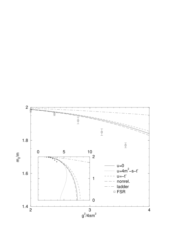
Figure 2: Ground state mass $m_{0}$ of the scalar theory as a function of the dimensionless coupling constant $g^{2}/4\pi m^{2}$ for $\mu/m=0.15$. The solid, dotted, dashed and long dashed lines correspond to the solutions with the spectral functions of Eqs. (7) to (10) respectively. The dashed-dotted line gives the ladder result, the boxes represent the non-perturbative results of Nieuwenhuis and Tjon [4]. The inset shows the evolution of the various solutions over the whole range of bound state energy values.

The inset of Fig. (2) shows the evolution of our solutions over the whole range of binding energies. As can be seen, the solution corresponding to the parametrization of Eq. (8) shows a double-valued structure with a lower branch where the binding energy decreases with increasing coupling. This is a consequence of the energy dependence of this choice, since replacing $s$ by $4m^{2}$, which corresponds to Eq. (9), renders the curve monotonically decreasing. It is however interesting to note that the lower branch does not start off at a coupling constant equal to 0 for $s=0$, as it is the case, for instance, for the Gross equation, (see below). Also the lower branch solution of the equal mass Klein-Gordon equation goes through 0 for $s=0$.

This qualitative difference to well known facts led us to investigate the $\mu$ dependence of our results. It was found that, from a value of the exchanged particles mass of about $\mu\sim 0.5$ on, the curves become monotonically decreasing even for the choice of Eq. (8). On the other hand, for $\mu\rightarrow 0$, the lower branch tends to $s=0$ for vanishing coupling.

This could have been immediately expected, since for $\mu=0$ the integral of Eq. (8) diverges, a reminiscent of the original infrared divergence of the box diagram. This is somehow a pity, since the case $\mu=0$, in the ladder approximation, corresponds to the Wick-Cutkosky model, which for $s=0$ admits analytic solutions in the form $\lambda=N(N+1)$ [13]. With the crossed box diagram included, all these solutions become degenerate at $\lambda=0$. We shall not comment any more on this subject, as we believe that further theoretical work is required in order to correctly account for the contribution of the crossed box diagram in the case $\mu=0$.

Nieuwenhuis and Tjon also give a detailed comparison of their results with those of various quasipotential equations. They considered the BSLT equation, the equal-time (ET) equation and the Gross equation [11]. Generally, these equations reduce the description from a 4-dimensional to a 3-dimensional one by making an ansatz for the propagators and the potentials involved. Specifically, the propagator factor of the Bethe-Salpeter equation in ladder approximation

$$S^{-1}(p)\Phi(p)=\frac{1}{(2\pi)^{4}}\,\int d^{4}p^{\prime}\,V(p-p^{\prime})\,\Phi(p^{\prime}),$$ (23)

(that is Eq. (1) after the Wick rotation) is replaced by the following forms in the various approaches (compare ref. [4]):

$$S_{\rm QPE}(p) \stackrel{{\scriptstyle\rm BSLT}}{{=}} \frac{1}{4\sqrt{\vec{p}^{2}+m^{2}}}\frac{2\pi\>\delta(p_{0})}{\vec{p}^{2}+m^{2}-\frac{1}{4}s},$$ (24)

$$\stackrel{{\scriptstyle\rm ET}}{{=}} \frac{1}{4\sqrt{\vec{p}^{2}+m^{2}}}\frac{2\pi\>\delta(p_{0})}{\vec{p}^{2}+m^{2}-\frac{1}{4}s}\times\left(2-\frac{s}{4(\vec{p}^{2}+m^{2})}\right)\!,$$ (25)

$$\stackrel{{\scriptstyle\rm Gross}}{{=}} \frac{1}{4\sqrt{s}\sqrt{\vec{p}^{2}+m^{2}}}\frac{2\pi\>\delta\left(p_{0}+\mbox{$\frac{1}{2}$}\sqrt{s}-\sqrt{\vec{p}^{2}+m^{2}}\right)}{\sqrt{\vec{p}^{2}+m^{2}}-\frac{1}{2}\sqrt{s}}.$$ (26)

In the potential function $V(p-p^{\prime})=K^{(1)}(p,p^{\prime},P)$ for the BSLT and ET equations, the time component is simply neglected:

$$V(p-p^{\prime})=g^{2}\frac{1}{(\vec{p}-\vec{p}^{\prime})^{2}+\mu^{2}},$$ (27)

whereas for the Gross equation $V$ takes the form

$$V(p-p^{\prime})=g^{2}\frac{1}{(\vec{p}-\vec{p}^{\prime})^{2}-(\omega-\omega^{\prime})^{2}+\mu^{2}},$$ (28)

with $\omega=\sqrt{\vec{p}^{2}+m^{2}}-\frac{1}{2}\sqrt{s}$ and $\omega^{\prime}=\sqrt{\vec{p}^{\prime 2}+m^{2}}-\frac{1}{2}\sqrt{s}$ .

In ref. [4] it was found that all the binding energies obtained in these quasipotential models are distributed between the energies of the FSR- and the ladder calculations. In Fig. (3) we compare our results with those of the equations specified above. For small coupling constants, we find that our binding energies, represented by the choice $u=0$ indicated in Fig (3), are remarkably close to those of the ET and Gross equation.

Since it is often conjectured that results like these may tend to support the validity of the instantaneous approximation, we would like to point out that this is true only for the specific model considered here. In fact, one can quickly convince oneself of the special nature of this approximate agreement by considering another specific case, where the involved particles would carry some sort of isospin. For the case already mentioned in Sect. 2, the contribution of the crossed box for a state of isospin 1 gets multiplied by a factor five, whereas the ladder terms remain unchanged. It can be seen in Fig. (3), that the corresponding curve even largely overshoots the Feynman-Schwinger points. The inset of Fig. (3) shows again the evolution of the curves over the whole range of binding energies and one can notice the unphysical lower branch of the Gross equation already mentioned above and discussed in ref. [4].

Let us finally notice that results quite similar to the ones presented here can also be obtained in a non-relativistic scheme. Details about this approach will be presented elsewhere [12].

Figure 3: Comparison of ground state masses obtained in various quasipotential equations with the results of the scalar theory in case of charge-less (solid line) and charged (dash-dotted line) particles. The latter one applies for a state of total isospin 1. Both curves correspond to the choice $u=0$ of Eq. (7). The boxes represent the non-perturbative Feynman-Schwinger results of ref. [4].

4.2 Excited states

In Fig. 4 we show the complete spectrum of lowest states for a spatial orbital angular momentum $l=0$ and an exchanged particle of mass $\mu=0.15$. The spectrum of the ladder approximation, on the left hand side, is very similar to the one of the Wick-Cutkosky model. There are normal and abnormal solutions, the latter ones corresponding to excitations in the relative time variable. For $s=0$ an approximate degeneracy appears. This can be traced back to the extra symmetry that occurs in the Wick-Cutkosky model, i.e. for $\mu=0$, when $s\rightarrow 0$ (O(5) instead of O(4)). Like in this model, the normal states tend to the correct non-relativistic limit when the coupling gets small, whereas the abnormal states exist only for larger values of the coupling constant. The only qualitative difference to the Wick-Cutkosky model is the fact that the different abnormal solutions do not tend to a common value of the coupling constant when the binding energy becomes small.

The spectrum gets considerably changed quantitatively by the inclusion of the crossed box diagram. On the right hand side of Fig. 4 we show the results for the energy independent choice $u=0$ of Eq. (7). First note the different scale in the coupling constant. Generally, the crossed box increases the binding energies for all states as compared with the ladder results.

Second, it has to be stated that we still find abnormal solutions with in fact similar properties as in the ladder approximation. Ever since the initial conjecture of Wick, it has been repeatedly claimed in the literature, that these abnormal states should be spurious consequences of the ladder approximation. The mere existence of these states beyond the ladder approximation is therefore already an interesting result per se.

Figure 4: Comparison of the complete spectrum of lowest states of the ladder approximation (left) and the one obtained by the inclusion of the crossed box diagram (right) for a spatial orbital angular momentum $l=0$. The solid lines give the normal solutions, dotted and dashed lines give abnormal solutions with even and odd time-parity, respectively.

As for the qualitative properties of the solutions, we see that the normal ones still behave normally, that is, they seem to have the correct weak binding limit. Also the abnormal solutions behave like in the ladder approximation in this limit, since they tend to different but larger values of the coupling constant. In the strong-binding limit however, the approximate degeneracy of states is severely lifted. This could have been expected, since the effect of the term on the right hand side of Eq. (7) is similar to the ladder term, Eq. (2), with a much higher effective mass $\mu$. An interesting feature is the fact that the abnormal solutions which are odd functions of relative time receive a more attractive contribution from the crossed box diagram than the even time-parity abnormal solutions. This is clearly seen in Fig. 4, where the odd time-parity solutions get shifted to the left, the even time-parity solutions to the right of the corresponding normal solutions. This even leads to the crossing of abnormal states, that in the ladder approximation would belong to different O(4) multiplets.

This crossing of states does not cause any numerical problems, since as outlined in Sect. 3, we calculate even- and odd time-parity solutions separately. There occurs however a problem for the even time-parity case. Since the normal solutions all tend to a value that is closer to zero than the limit of the abnormal solutions, the former ones necessarily cross some of the latter ones, if they initially belonged to a higher O(4) multiplet. This leads to a perturbation of the eigenvalues near the crossing region, which can be clearly seen from Fig. (4) in the case of the two positive time-parity abnormal solutions. The effect is in principle also present in the ladder approximation, but it seems somehow less pronounced there. In fact, taking a closer look at the crossing region, one finds rather a repulsion of the two solutions, with no real crossing taking place. In this region, it is obviously not possible to identify the two solutions due to configuration mixing. It is only by the smooth continuation of the curves after the crossing, that the solutions were identified in order to draw the graph of Fig. 4. The curve for the abnormal solution after the crossing is however not expected to be meaningfull anymore, since it gets repeatedly perturbed by all the normal states crossing it.

5 Conclusion

In this work, we have studied the contribution due to crossed two-boson exchange to the binding energy of a system made of two distinguishable particles. This was done in the framework of the Bethe-Salpeter equation. The present work completes that one by Nieuwenhuis and Tjon for the lowest $l=0$ state, allowing one to determine what is the role of the simplest crossed-boson exchange contribution among all those included in their work. For the range of coupling constants where a comparison is possible, this contribution is rather well determined and accounts for roughly half of the total effect, the discrepancy tending to increase with the coupling. This is consistent with the expectation that the role of multi-boson exchanges not included here should increase similarly. The result is however somewhat disturbing. It implies that the convergence of the Bethe-Salpeter approach in terms of an expansion of the interaction kernel in the coupling constant is likely to be slow. We obviously assumed that the comparison is meaningful, namely the results of Nieuwenhuis and Tjon exclude effects from self-energy or vertex corrections ignored here.

Amazingly, our results, which include crossed two-boson exchange contributions, are close to those obtained with the instantaneous approximation, where these contributions are absent. This confirms a theoretical result obtained in a non-relativistic scheme [5]. Like there, the specific character of this coincidence is demonstrated by the consideration of a model with “charged” bosons, which leads to a different conclusion, showing that the validity of the instantaneous approximation is limited to the Born approximation.

We have looked at excited states, including abnormal ones. Our results are partly academic. The effect due to the simplest crossed-boson exchange is so large that one has to seriously worry about higher order crossed-boson diagrams. Interesting features nevertheless show up. There is no tendancy for abnormal states to disappear, as sometimes conjectured in the literature. Their energy is differently affected, depending on the parity of the states under a change in the sign of the relative time coordinate.

We scarcely considered the case of an exchanged boson with zero mass, which would be most interesting in view of possible applications to QED. This case supposes further theoretical work to deal with the divergences that appear. Getting rid of the $\alpha^{3}\,{\rm log}\alpha$ corrections to the binding energy obtained in the ladder approximation for the case of scalar neutral bosons should be easily achieved. Removing the corrections $\alpha^{3}$, which are absent in results obtained from the Dirac or Klein-Gordon equations, is more delicate. In any case, the difficulty has a somewhat general character and is not pertinent to the present approach.

Another development concerns the understanding of the remaining discrepancies with the FSR results. Estimating the contribution of crossed three-boson exchange is not out of reach with some approximations. The net effect is unclear however. In the non-relativistic case, at the order $(\frac{1}{m})^{0}$, it is expected to vanish as a result of a cancellation with a contribution due to the renormalization of the interaction [5]. It remains the possibility that the higher order corrections, which seem to be responsible for a slight extra binding in present results, have their role slowly increased when the treatment of the problem becomes more complete.

References

- [1] Salpeter, E.E. and Bethe, H.A.: Phys. Rev. 84, 1232 (1951).
-
[2]
Todorov, I.T.: Phys. Rev. D3, 2351 (1971);
Brezin, E., Itzykson, C. and Zinn-Justin, J.: Phys. Rev. D1, 2349 (1970);
Friar, J.L.: Phys. Rev. C22, 796, (1980);
Gross, F.: Phys. Rev. C26, 2203 (1982);
Neghabian, A.R. and Glöckle, W.: Can. J. Phys. 61, 85 (1983). - [3] Feldman, G., Fulton, T. and Townsend, J.: Phys. Rev. D7, 1814 (1973).
- [4] Nieuwenhuis, T. and Tjon, J.A.: Phys. Rev. Lett. 77, 814 (1996).
- [5] Amghar, A. and Desplanques, B.: to be published.
- [6] Mandelstam, S.: Phys. Rev. 115, 1741 (1959).
- [7] Itzykson, C. and Zuber, J.B.: Quantum Field Theory. McGraw-Hill International Editions (1985).
- [8] Chemtob, M., Durso, J.W. and Riska, D.O.: Nucl. Phys. B38, 141 (1972).
- [9] Schwartz, C.: Phys. Rev. 137, 717 (1965).
- [10] Nieuwenhuis, T. and Tjon, J.A.: Few Body Systems 21, 167 (1996).
-
[11]
Blankenbecler, R. and Sugar, R.: Phys. Rev. 142,
1051 (1966),
Logunov, A.A. and Tavkhelidze, A.N.: Nuovo Cimento 29, 380 (1963);
Hummel, E. and Tjon, J.A.: Phys. Rev. C 49, 21 (1994),
Devine, N.K. and Wallace, S.J.: Phys. Rev. C 51, 3223 (1995);
Gross, F.: Phys. Rev. 186, 1448 (1969),
Gross, F.: Phys. Rev. D 10, 223 (1974). - [12] Desplanques, B., Theußl, L. and Amghar, A.: in preparation.
-
[13]
Wick, G.C.: Phys. Rev. 96, 1124 (1954);
Cutkosky, R.E.: Phys. Rev. 96, 1135 (1954).