Strange matter in the string-flip model

Abstract

We employ variational Monte Carlo methods to study the transition to strange matter in a simple one-dimensional string-flip model with two flavors and two colors of quarks. The dynamics of the system are described in terms of a many-body potential that confines quarks within hadrons, yet enables the hadrons to separate without generating unphysical long-range van der Waals forces. The model has “natural” low- and high-density limits: it behaves as a system of isolated hadrons at low density and as a Fermi gas of quarks at high density. We show that the system exhibits a transition to strange matter characterized by an increase in the length-scale for confinement. Yet the small increase at the transition region — of only ten percent — suggests that clustering correlations remain strong well into the strange-matter domain. Our results put into question descriptions of strange matter in terms of noninteracting, or weakly interacting, quarks.

I INTRODUCTION

The possible existence of stable strange matter — more stable even than ⁵⁶Fe — is fascinating indeed [1]. That this scenario is plausible at high baryon density is simple to understand: for two-flavor (up and down) matter the Fermi energy becomes so large that the addition of strange quarks becomes energetically favorable, in spite of the larger strange-quark mass. The existence of strange matter should have a dramatic impact on fields ranging from astrophysics and cosmology to nuclear and particle physics. Indeed, it is widely accepted that the high-density environment at the core of neutron stars constitutes a fruitful ground for the formation of quark matter. Moreover, the recent proposal of a “spin-up” phase in the timing structure of pulsars, speculated to signal the transition from hadronic to quark matter, makes the detection of this exotic phase of matter within observational reach [2]. These astronomical observations complement terrestrial searches for strange matter which have improved considerably, and will continue to do so, with the commission of new powerful relativistic heavy-ion colliders [3].

The theoretical study of strange matter has traditionally been conducted in two different pictures: one using a hadronic model [4] — similar to ordinary nuclei — where the fundamental degrees of freedom are mesons and baryons, another using a quark model [5, 6] consisting of massless, noninteracting quarks confined inside a bag (note that the inclusion of a finite strange-quark mass and a perturbative treatment of QCD does not seem to change the qualitative picture). Presumably a description of strange matter in terms of mesons and baryons is well motivated in the low-density regime where clustering correlations remain important. Alternatively, strange matter viewed in terms of a Fermi gas of quarks might be appropriate in the high-density domain, as now the average interquark separation becomes considerably smaller than the length-scale for confinement. This division, however, seems arbitrary. Indeed, it is not at all clear how and at what density the “transition” should be made from a hadronic- to a quark-matter description. Moreover, there might be certain regions where none of the pictures could be physically realized. For example, one could imagine the existence of an intermediate-density phase characterized by an increase in the length-scale for confinement (“swollen” baryons) but also in which clustering correlations remain important. Perhaps the most serious difficulty encountered in studying the density dependence of strange matter is how to model a system that has quarks confined inside color-neutral hadrons at low density but free quarks at high density. The divorce of the two pictures is further reinforced by the difficulty of treating quark confinement: how can quarks be confined inside hadrons, yet the hadrons separate without generating long-range van der Waals forces? We offer no new insight into this difficult problem; rather, we argue here that it is useful to consider an effective model which interpolates between a hadron- and a quark-based description.

To do so we rely on the string-flip model. One strength of this model is that the evolution of the system from a low-density hadronic phase to a high-density quark phase is dynamical rather than through the introduction of artificial parameters. Yet the string-flip model employed here is simple and its predictions should be taken with caution. Still, we trust that some of the qualitative features obtained from our analysis will have a direct correspondence to those made in more sophisticated models. The string-flip model used here is an offspring of the original one-dimensional model proposed by Lenz and collaborators [7] and applied for the first time to nuclear matter by Horowitz, Moniz, and Negele [8]. Since then the model has been generalized to three dimensions and internal degrees of freedom (such as color) have been incorporated to study a variety of ground state properties [9, 10, 11, 12]. All these models represent simple — yet realistic — many-body generalizations of the non-relativistic constituent quark model [13]. The cornerstone of the string-flip model is the many-body nature of the potential which allows quark confinement within hadrons, while enabling the hadrons to separate without generating long-range van der Waals forces [14].

There are several questions that we will try to answer in this paper. First, how does the length-scale for quark confinement evolve as the density of the system increases and how is this evolution affected by the presence of strange quarks? Second, how does the many-body (confining) potential modifies the transition to strange matter relative to the predictions of a Fermi-gas estimate; do clustering correlations remain important at the transition density or has the system dissolved into a collection of noninteracting quarks? Finally, what can one learn about the dynamic response of the system through a study of two-body correlations between quarks.

Our paper has been organized as follows. In Sec. II we introduce the particular version of the string-flip model used here to compute a variety of ground-state properties of strange matter. Variational Monte-Carlo results are presented in Sec. III and compared against some useful limiting cases. Finally, our conclusions and outlook are offered in Sec. IV.

II Formalism

We compute the properties of strange matter in a string-flip model that has constituent quarks — interacting through a many-body potential — as the fundamental degrees of freedom. The many-body potential used here is explicitly symmetric in all quark coordinates, confines quarks within hadrons, and enables the hadrons to separate without generating long-range van der Waals forces. In this paper we use the simplest form of this model that can describe the basic quark structure of strange matter. In this version quarks are constrained to move in one spatial dimension and have only two SU(2)-like intrinsic degrees of freedom: color and flavor. The color — a global, rather than a local — quantum number can be either red or blue (with red+blue=“white”) and the flavor either up or strange. Thus, “color-neutral hadrons” are represented as two-quark composites coming in three different varieties: nucleon ($uu$), lambda ($us$), and cascade ($ss$).

A Many-quark Potential

The Hamiltonian for a system of $N$ quarks moving in one-spatial dimension under the influence of the many-body potential $V$ is given by

$$H=T+V=\sum\limits^{N}_{i=1}\frac{p^{2}_{i}}{2m_{i}}+V(x)\;.$$ (1)

The first step in constructing the $N$-body potential $V(x)$ is the pairing of all $N$-quarks into $A\!=\!N/2$ color-neutral clusters, irrespective of quark flavor. This procedure results in a total of $A!$ possible configurations. For each of these configurations one now introduces a flux-tube energy:

$$V_{n}(x)=\frac{1}{2}k\sum\limits^{A}_{i=1}\left(r_{i}^{(n)}-b_{i}^{(n)}\right)^{2}\;,$$ (2)

where $r_{i}^{(n)}$ and $b_{i}^{(n)}$ are the positions of the red and blue quarks within the $i$th cluster, and $k$ is the strength of the confining potential (which here has been assumed harmonic). Finally, the many-body potential is obtained by demanding that the pairing of quarks into color-neutral hadrons be optimal. That is, that the potential be the minimum value of $V_{n}$ among all the $A!$ possible pairings,

$$V(x)\equiv\min_{n=1}^{A!}\Big{\{}V_{n}(x)\Big{\}}\;.$$ (3)

Note that in what follows we adopt units in which $\hbar$, the spring constant $k$, and the up-quark mass are all equal to one while for the constituent strange-quark mass the canonical value of $m_{s}/m_{u}=1.6$ is used.

The minimum prescription described above ensures that the potential is, indeed, symmetric under the exchange of identical quarks. Moreover, no long-range van der Waals forces are generated in the model as the force saturates within each individual hadron. In this way residual interactions between hadrons involve the possibility of quark-exchange (when the strings flip) and the Pauli exclusion principle between identical quarks. Finally, as it is possible for all pairings to change as one moves a single quark, the potential is truly an $N$-body operator; it cannot be reduced to a conventional sum of two-body terms. The global minimization procedure should be taken among all possible $A!$ configurations, which rapidly becomes unmanageable; for $A\!=\!40$ (the canonical value used in our simulations) the total number of possible configurations is close to $10^{48}$. Fortunately, because we have restricted the problem to one spatial dimension, finding the optimal solution scales linearly — not exponentially — with the number of quarks. (In reality the solution to the pairing problem scales only with the cube of the number of quarks [11, 15]. To our knowledge a polynomial solution to the three-quark assignment problem has yet to be found).

To generate the desired $A$ configurations one starts by ordering the red and blue quarks, independently, in a one-dimensional box of length $L$ (note that the concept of “order” is meaningful only in one spatial dimension). The first of these configurations is obtained by mapping the first red quark into the first blue quark, the second red quark into the second blue quark, and so on until finally the last red quark is paired with the last blue quark. Similarly, the second of these configurations is generated by mapping the first red quark into the second blue quark and then continuing the assignments sequentially. One continues this procedure until in the last configuration the first red quark is mapped into the last blue quark. That is,

$$r_{1}\leftrightarrow b_{1}\;;\;r_{2}\leftrightarrow b_{2}\;;\; \ldots \;;\;r_{A}\leftrightarrow b_{A}\;,\quad\mbox{or}\quad V_{1}(x)=\frac{1}{2}\sum\limits^{A}_{i=1}\left(r_{i}-b_{i}\right)^{2}\;,$$

$$r_{1}\leftrightarrow b_{2}\;;\;r_{2}\leftrightarrow b_{3}\;;\; \ldots \;;\;r_{A}\leftrightarrow b_{1}\;,\quad\mbox{or}\quad V_{2}(x)=\frac{1}{2}\sum\limits^{A}_{i=1}\left(r_{i}-b_{i+1}\right)^{2}\;,$$

$$\ldots$$

$$r_{1}\leftrightarrow b_{A}\;;\;r_{2}\leftrightarrow b_{1}\;;\; \ldots \;;\;r_{A}\leftrightarrow b_{A-1}\;,\quad\mbox{or}\quad V_{A}(x)=\frac{1}{2}\sum\limits^{A}_{i=1}\left(r_{i}-b_{i+A-1}\right)^{2}\;.$$

The potential energy is then selected to be the minimum among the $A$ configurations:

$$V(x)=\min\Big{\{}V_{1}(x),V_{2}(x),\ldots,V_{A}(x)\Big{\}}\;.$$ (4)

Despite the relative simplicity of the model a clear picture of the quark dynamics emerges in the low- and high-density phases of the system. In the low-density phase the confinement scale — a typical distance between quarks within a hadron in free space — is much smaller than the inter-hadron separation. Since the potential saturates within each individual hadron, quark exchange is suppressed and the system resembles a collection of noninteracting nucleons. In the high-density phase, however, the confinement scale becomes larger than the inter-hadron separation making string rearrangement dominant. By then the potential energy is unimportant relative to the kinetic energy and the system resembles a free Fermi gas of quarks.

B Fermi Gas of Quarks

In this section we compute ground-state properties of a simple Fermi-gas model of quarks in order to establish a baseline against which the predictions of the string-flip model may be compared. The total energy of a one-dimensional free Fermi gas of quarks is simply the sum of the kinetic energies of the two flavors

$$\frac{T_{FG}}{N}(\rho,\sigma)=(1-\sigma)+\frac{k_{F}^{2}}{6}(1-\sigma)^{3}+m_{s}\sigma+\frac{k_{F}^{2}}{6m_{s}}\sigma^{3}\;;\quad k_{F}\equiv\frac{\pi}{2}\rho\;,$$ (5)

where the strangeness-per-quark parameter $\sigma\equiv|S|/N$ and the density $\rho$ have been introduced. However our results will be presented in terms of the more conventional strangeness-per-baryon ratio $f_{s}=|S|/A$ and the relative density $\rho/\rho_{c}$ where $\rho_{c}$ is defined below. Note that $k_{F}$ is the Fermi momentum of the system in the limit of $|S|\equiv 0$. The strangeness-per-quark ratio is determined by demanding that the total energy of the system be minimized with respect to $\sigma$ at fixed baryon density. That is,

$$\left(\frac{\partial T_{FG}}{\partial\sigma}\right)_{\rho}\!=0=-1-\frac{k_{F}^{2}}{2}(1-\sigma)^{2}+m_{s}+\frac{k_{F}^{2}}{2m_{s}}\sigma^{2}\;.$$ (6)

The above condition represents chemical equilibrium meaning that the chemical potential of both species must be equal. The solution to this quadratic equation is simple and from it one obtains the strangeness-per-quark ratio as a function of the density of the system

$$\sigma(\rho)=\frac{m_{s}k_{F}-\sqrt{m_{s}\Big{[}2(m_{s}-1)^{2}+k_{F}^{2}\Big{]}}}{(m_{s}-1)k_{F}}\;.$$ (7)

Although not explicitly stated, the above equation is valid only above a critical density $\rho_{c}$ below which the strangeness-per-quark ratio vanishes. This is due to the fact that below $\rho_{c}$ it is not yet energetically favorable to introduce strange quarks into the system. The critical density is given by

$$\rho_{c}=\frac{2}{\pi}\sqrt{2(m_{s}-1)}\approx 0.697\;.$$ (8)

Finally, the Fermi-gas energy is obtained by substituting Eq. (7) into Eq. (5), i.e.,

$$T_{FG}(\rho)=T_{FG}\Big{(}\rho,\sigma(\rho)\Big{)}\;.$$ (9)

Another observable useful in characterizing the transition from hadronic- to quark-matter is the two-body correlation function. This function represents the ground-state probability of finding a pair of quarks at a fixed separation. That is,

$$\rho_{2}(r)=\left\langle\sum_{i<j}\delta\Big{(}r-|r_{i}-r_{j}|\Big{)}\right\rangle=\sum_{q}e^{iqr}\sum_{k_{1},s_{1};k_{2},s_{2}}\left\langle C^{\dagger}_{k_{2}+q,s_{2}}C^{\dagger}_{k_{1}-q,s_{1}}C_{k_{1},s_{1}}C_{k_{2},s_{2}}\right\rangle\;,$$ (10)

where $C^{\dagger}_{k,s}$($C_{k,s}$) represents a quark creation(annihilation) operator with momentum $k$ and (SU(2)-like) color quantum number $s$. The above two-body operator is easily evaluated in the Fermi-gas limit to obtain

$$\rho_{2}(r)\propto g_{FG}(r)=1-\frac{1}{2}\left(\frac{\sin(k_{F}r)}{k_{F}r}\right)^{2}\;.$$ (11)

Note that we have introduced the function $g_{FG}(r)$ which is simply the two-body correlation function normalized to one at large distances. This function is sensitive only to Pauli correlations. The second term in Eq. (11) — with its corresponding 50% reduction at the origin — accounts for this fact.

C Variational Wavefunction

In this section we compute ground-state properties of the string-flip Hamiltonian of Eq. (1) using a variational Monte Carlo approach. For a system of $N$ quarks moving in a one-dimensional box of length $L$ the one parameter variational wavefunction has the form

$$\Psi_{\lambda}=e^{-\lambda U(x)}\Psi_{FG}(x)\;,$$ (12)

where $\lambda$ is the variational parameter and $\Psi_{FG}$ represents a free Fermi-gas wavefunction comprised of the product of four Slater determinants; one for each color-flavor combination. For example, the one-dimensional Slater determinant for the “red-up” combination is of the form [8, 16]

$$\Phi_{\rm FG}^{(red-up)}(x)=\prod\limits_{i<j}\sin\left[\frac{\pi}{L}(r^{up}_{i}-r^{up}_{j})\right]\;.$$ (13)

The Fermi-gas wavefunction is exact for a system of fermions with no correlations other than those generated by the Pauli exclusion principle, while the exponential portion of the variational wavefunction — symmetric under the exchange of identical quarks — characterizes the amount of clustering in the ground state. Here we have introduced the “quasi-potential”

$$U(x)=\alpha_{uu}V_{uu}(x)+\alpha_{us}V_{us}(x)+\alpha_{ss}V_{ss}(x)\;,$$ (14)

where $V_{uu}$, $V_{us}$, and $V_{ss}$ are the portions of the many-body potential that reside in nucleons, lambdas, and cascades respectively; that is: $V(x)=V_{uu}(x)+V_{us}(x)+V_{ss}(x)$. The constants $\alpha_{uu}$, $\alpha_{us}$, and $\alpha_{ss}$ correct for the sizes of the different hadrons and are thus proportional to the ratio of the reduced mass of the corresponding hadron to that of the nucleon:

$$\alpha_{uu}=1\;,\quad\alpha_{us}=\sqrt{\frac{2m_{s}}{1+m_{s}}}\approx 1.109\;,\quad\mbox{and}\quad\alpha_{ss}=\sqrt{m_{s}}\approx 1.265\;.$$ (15)

In the low-density phase — or in a phase with various noninteracting hadrons — the variational wavefunction becomes exact in the limit of $\lambda\rightarrow 1/\sqrt{2}$ (value of the oscillator parameter for isolated two-quark clusters). Similarly, in the high-density limit where the potential is unimportant, the variational wavefunction reproduces exactly that of a free Fermi gas of quarks in the limit of $\lambda\rightarrow 0$.

D Metropolis Monte Carlo

An additional advantage of using such a simple variational wavefunction is that the expectation value of the kinetic and potential energies are not independent [8, 16]. Indeed, the expectation value of the kinetic energy, difficult to simulate because of its derivatives, is easily related to the expectation value of the potential energy. That is,

$$\langle\Psi_{\lambda}|T|\Psi_{\lambda}\rangle=T_{FG}+2\lambda^{2}\langle\Psi_{\lambda}|V|\Psi_{\lambda}\rangle\;,$$ (16)

where $T_{FG}$ is the kinetic energy of a one-dimensional free Fermi gas given in Eq. (5). The minimum value of the kinetic energy is attained in the Fermi-gas limit. The additional term in the above expression — $2\lambda^{2}\langle V\rangle_{\lambda}$ — represents the increase in the kinetic energy above the Fermi-gas limit due to the presence of clustering correlations. While the kinetic energy disfavors such correlations the potential energy favors them, at least at low density. The dynamic competition between the kinetic and potential energies will yield an optimal value for the variational parameter for any given density and strangeness-to-baryon ratio. The optimal value of the variational parameter is thus obtained by minimizing the total energy of the system:

$$\langle E\rangle_{\lambda\rho\sigma}=T_{FG}(\rho,\sigma)+(2\lambda^{2}+1)\langle V\rangle_{\lambda\rho\sigma}\;.$$ (17)

As promised, to compute the ground-state expectation value of the energy we need only compute the expectation value of the potential energy, which we accomplish using Monte-Carlo methods. Using the algorithm of Metropolis et al., it can be shown [17] that the expectation value of the potential energy can be obtained by performing a suitable average of the form

$$\langle V\rangle=\lim_{M\rightarrow\infty}\frac{1}{M}\sum\limits_{m=1}^{M}V(x_{m})\;,$$ (18)

where the sequence of points $\{x_{m}\}$ are distributed according to the square of the variational wavefunction. It then becomes a simple — yet computationally-intensive – task to extract the optimal variational parameter that minimizes the energy of the system for each value of the density and for each number of strange quarks.

III Results

We start this section by displaying in Fig. 1 the energy-per-quark of the system as a function of the variational parameter for a variety of strangeness-per-baryon ratios at a fixed density of $\rho=1.2$ (or $\rho/\rho_{c}=1.72$; recall that $\rho_{c}=0.697$ represents the critical density for the transition to strange matter in a Fermi-gas model). Note that all the calculations reported in this work have been effected at the fixed baryon number of $A\!=\!40$. The plot shows the, time-consuming, procedure used to extract the optimal variational parameter, the strangeness-per-baryon ratio, and the energy-per-quark at a fixed value of the density. Indeed, for every value of $f_{s}$ the optimal variational parameter is extracted as the point at which the derivative of the energy with respect to $\lambda$ vanishes. For example, Fig. 1 shows that, for this density, the minimum energy-per-quark decreases when the number of strange quarks goes from 8 ($f_{s}=0.2$) to 24 ($f_{s}=0.6$) but increases again if more strange quarks ($f_{s}=1.0$) are added to the system. The optimal value of $\lambda$ at a density of 1.2 must therefore be extracted when the system contains 24 quarks. One then repeats this procedure for all densities.

The optimal variational parameter as a function of density is displayed in Fig. 2. Variational results for strange (circles) and non-strange nuclear (squares) matter are shown; the solid and dashed lines are smooth interpolations to the data. As expected, the variational parameter evolves from the isolated-hadron limit of $\lambda_{0}\!=\!1/\sqrt{2}$ at low density towards the Fermi-gas limit of $\lambda=0$ at high density. It is important to stress that the decrease in $\lambda$ with density — with the corresponding increase in the length-scale for confinement — is a prediction of the model. At the transition density to strange matter, $\rho=0.9$ or $\rho\!=\!1.3\rho_{c}$, both sets of results start to differ, indeed strange matter favors stronger clustering correlations because of the larger mass of the strange quark. In this way we obtain one of the most important results of our simulations: at the transition density the length-scale for confinement (proportional to $\lambda^{-1/2}$) has increased by only 10%, relative to its isolated-hadron value. At this density — and well into the strange-matter region — clustering correlations remain strong and the system is far from becoming a collection of noninteracting, or weakly interacting, quarks.

The equation of state of the system — the energy-per-quark as a function of density — is displayed in Fig. 3. The variational results (circles joined by the solid line) evolve from the isolated-hadron to the Hartree-Fock limit. The importance of clustering correlations at low density is irrefutable. Indeed, a Hartree-Fock estimate of the ground-state energy (triangles joined by the dotted line) diverges at low densities as $E_{HF}\!\sim\!\rho^{-3/2}$. Moreover, although clustering correlations will eventually become unimportant, the energy of the system remains about 5% larger than the Fermi-gas result even at the highest shown density. This picture also emphasizes that at the transition region, depicted by the point at which the nuclear calculation (squares joined by the dashed line) departs from the strange-matter calculation, clustering correlations remain strong. Finally, we have included “hypernuclear” results (diamonds joined by dot-dashed lines) obtained by maintaining the variational parameter fixed at its free-space value ($\lambda\!=\!\lambda_{0}$ at all densities). In this approximation baryons are treated as incompressible quark composites. It can be seen that for the range of densities probed in our simulations, baryon “swelling” — the increase in the length scale for confinement with density — seems to play an insignificant role, making the hypernuclear limit an excellent approximation to the variational results.

Even more insensitive to baryon swelling is the strangeness-per-baryon ratio displayed in Fig. 4. Indeed, aside from a minor delay in the transition to strange matter relative to the Fermi-gas estimate, the strangeness-per-baryon ratio seems insensitive to most details of the many-body potential. Clustering is the only feature that seems to affect $f_{s}$. Yet even the Hartree-Fock estimate agrees with the variational result for $\rho\!>\!1.8\,\rho_{c}$ despite the fact that at this density the Hartree-Fock result overestimates the variational energy by almost 20%.

We continue by presenting results for the two-body correlation function. While providing a useful characterization of the transition from hadronic- to quark-matter, this observable also appears to be more sensitive to the fine details of the model. In Fig. 5 we display the evolution of the “up-up” correlation function with density. The upper-left-hand panel shows the system at very low density where clustering correlations remain strong. Thus, the two-body correlation function at short-to-intermediate distances is accurately represented by the Gaussian behavior of the wavefunction of an isolated nucleon (depicted by the dashed line and barely visible in the figure). Also shown is the two-body correlation function for a free Fermi-gas of quarks [solid line; see also Eq. (11)]. Evidently, Pauli correlations play an insignificant role in this very dilute system. As the density increases to $\rho\!=\!0.6$, $f_{s}$ remains at zero but nucleon swelling — the increase in the length-scale for confinement — is now discernible as indicated by the deviation from the isolated-nucleon result. Moreover, the correlation function now displays the typical long-distance oscillations, albeit much stronger, of a Fermi-gas system. In the third panel ($\rho=1$) the system displays features related to both — hadronic and Fermi-gas — limits: an enhanced correlation at short distances and a rapid “healing” towards the Fermi-gas limit at larger distances. Finally, the last panel shows that the evolution to the Fermi-gas limit is now complete, in spite of a value for the variational parameter which, at 50% of its isolated-hadron value, is still large.

In addition to the up-up correlation function one can measure two-body correlations for the other two flavor combinations as displayed in Fig. 6. The upper two panels show, as a result of the Pauli principle not being operative between quarks of different flavors, a featureless “up-strange” correlation function. In contrast, the strange-strange correlation function at intermediate density (lower-left panel) shows characteristics that cannot be associated exclusively with either those of isolated clusters or a Fermi gas but contains some features of both. At the largest density shown in the figure ($\rho\!=\!2$) the transition to the Fermi-gas limit seems now complete.

So why the emphasis on the two-body correlation function? As stated earlier, the two-body correlation function is a useful observable for characterizing the transition from hadronic to quark matter. Moreover, it displays clearly the dynamic interplay between clustering and Pauli correlations. Yet its real appeal stems from its relation to the dynamic response of the system. Indeed, the two-body correlation function is related to the Fourier transform of the static structure factor:

$$\frac{1}{N}S(q)=1+\rho\int_{-\infty}^{\infty}e^{-iqr}\Big{(}g(r)-1\Big{)}dr=1+\rho\int_{0}^{\infty}2\cos(qr)\Big{(}g(r)-1\Big{)}dr\;,$$ (19)

with the static structure factor, itself, being defined as the integrated sum of the dynamic response function,

$$S(q)=\int_{0}^{\infty}S(q,\omega)\,d\omega\;.$$ (20)

As a preview of future work, devoted to the study of the exact Euclidean response of the system and its analytic continuation into real time, we focus on the static structure factor known as the Coulomb sum. In Fig. 7 we display the Coulomb sum as a function of the momentum transfer at the low density of $\rho=0.2$. The dashed line represents the response of free Fermi gas of quarks; evidently well below the variational result. This behavior suggests that at these momentum transfers both quarks in a hadron respond coherently. Yet the coherence is incomplete, as the response of the system at low $q$ is below that of a free Fermi gas of nucleons (solid line). Some of the coherence is lost because of the intrinsic quark structure of the nucleon: the nucleon “survival” probability is proportional to its elastic form factor. Note that the very large “spike” at exactly $q=2k_{F}$ is an artifact of the “rigidity” imposed by the Pauli exclusion principle in one spatial dimension. We are currently in the process of applying familiar nuclear techniques, such as the impulse approximation, to gain insight into the physics of this fundamental problem. Preliminary results for a simplified version of the model have been published in Ref. [18].

IV Conclusions and Outlook

We have employed variational Monte Carlo techniques to compute ground-state properties of strange matter in a one-dimensional string-flip model with two flavors and two colors of quarks. In this simplified model baryons are color-neutral, two-quark composites. We have used a many-body potential that confines quarks within baryons yet enables the hadrons to separate without generating unphysical long-range forces as the confining force saturates within each individual hadron. The many-body nature of the potential entails a difficult optimization problem: how to pair $N$ quarks into $A\!=\!N/2$ color-neutral clusters so that the overall flux-tube energy is minimized. For the general three-dimensional case this problem involves searching among $A!$ distinct configurations, a task that becomes prohibitely costly even for small systems. The one-dimensional case studied here is special as one can restrict the search to only $A$ configurations. In this manner we were able to simulate systems with up to $N=80$ quarks (note that in an exhaustive routine one would have to search among close to $10^{48}$ configurations!). In this paper we have used, for the sake of computational expediency, the simplest string-flip model that can describe the basic quark structure of strange matter.

The crucial feature of all string-flip models is the need to determine an optimal grouping of quarks into hadrons. This need alone yields two natural limits for the model: a hadronic limit at low density and a Fermi-gas limit at high density. The system thus exhibits a transition from hadronic matter, where clustering correlations dominate, to quark matter, where only Pauli correlations remain. This is one of the greatest advantage of the model: the transition from hadronic- to quark-matter is dynamic, as there is no need to resort to ad-hoc prescriptions. The main goal of this paper was the characterization of the transition to strange matter; does the transition happens at a density at which the system has already dissolved into a collection of “free” quarks or do clustering correlations remain strong? In our model the transition to strange matter occurred at a density of approximately $\rho\!=\!1.3\rho_{c}$ ($\rho_{c}$ was defined as the transition density predicted by the free Fermi-gas estimate). Thus, the many-body potential delays the transition relative to that of a free Fermi gas. More interestingly, the length-scale for confinement increased at the transition by merely 10% of its isolated-hadron value and in fact clustering correlations remained strong well into the transition region. Indeed, we observed that ground-state properties computed in the “hypernuclear” limit were almost identical to those predicted by the variational approach. In sharp contrast, a Hartree-Fock estimate — which includes Pauli but not clustering correlations — predicted a much larger value for the transition density and an energy-per-quark that overestimates (at the transition density) the variational estimate by about 20%. Thus — on the basis of our findings — we conclude that the behavior of the system at the transition density is well reproduced by a hadronic model with no baryon swelling, but not by one that ignores clustering correlations.

In the future we plan to extend this calculation in several directions. First, we need to refine the many-body potential in order to study the possibility of stable, or absolutely stable, strange matter. The string-flip potential used here seems to account for the short- and intermediate-range structure of the nucleon-nucleon potential. Indeed, the Pauli principle between quarks generates a short-range repulsion between clusters while quark-exchange generates, at least part of, the intermediate-range attraction. What is missing from the model is the long-range (pion) tail. One could introduce a phenomenological long-range part to the potential constrained to reproduce the equation of state of nuclear matter. With this model for the potential in hand one could then predict the stability, or lack-thereof, of strange matter. Second, while undoubtedly challenging, simulating three-dimensional strange matter with three flavors and three color of quarks is now within computational reach. Finally, one should attempt to calculate the dynamic response of the system. We wish to understand — as a function of density and of the momentum transfer — when do leptons scatter from hadrons and when do they scatter from the individual quarks. We have offered a preliminary answer to this question. By computing the two-body correlation function, and from it the Coulomb sum, we observed that the response of the system at small momentum transfers was well above the response of a free Fermi gas of quarks. This suggested that all the quarks in the hadron respond coherently. Yet we saw that the coherence was incomplete, as the response was below that of a Fermi gas of nucleons. We attributed this loss of coherence to the internal quark structure of the hadron. How this picture can be reconciled with more sophisticated models of the reaction, such as in the impulse approximation, remains an interesting open question. In summary, we have shown that in spite of their deceiving simplicity, string-flip models of hadronic matter display rich behavior that could yield valuable insights into the physics of strange matter.

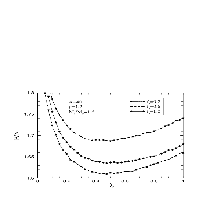
FIG. 1.: Energy-per-quark as a function of the variational parameter for a variety of strangenes-per-baryon ratios. The number of baryons has been fixed at $A\!=\!40$ and the quark density at $\rho=1.2$ ($\rho/\rho_{c}\!=\!1.72$).

FIG. 2.: Variational parameter as a function of density for nuclear (squares) and strange (circles) matter.

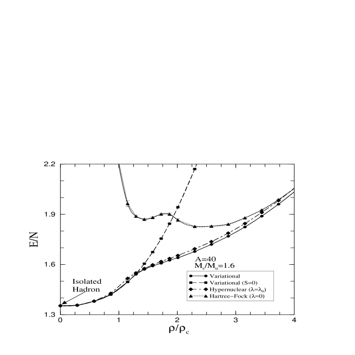
FIG. 3.: Energy-per-quark as a function of density. See the text for details.

FIG. 4.: Strangeness-per-baryon ratio as a function of density. See the text for details.

FIG. 5.: Two-body up-up correlation function for a variety of densities.

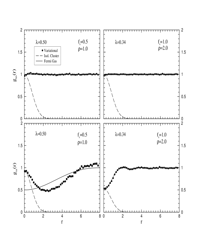
FIG. 6.: Two-body up-strange and strange-strange correlation functions for a variety of densities.

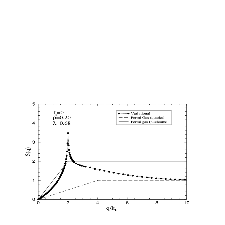
FIG. 7.: Coulomb sum as a function of density in units of the Fermi momentum.

- [1] Two excellent recent reviews on strange-quark matter are: Carsten Greiner and Jürgen Schaffner-Bielich, “Physics of Strange Matter”, nucl-th/9801062; Jes Madsen, “Physics and Astrophysics of Strange Quark Matter”, astro-ph/9809032.
- [2] N.K. Glendenning, S. Pei, and F. Weber, Phys. Rev. Lett. 79, 1603 (1997).
- [3] T.A. Armstrong et al., Phys. Rev. C 59, R1829 (1999), and references therein.
- [4] J. Schaffner, C.B. Dover, A. Gal, C. Greiner, and H. Stöcker, Phys. Rev. Lett. 71, 1328 (1993).
- [5] E. Witten, Phys. Rev. D 30 (1984) 272.
- [6] E. Farhi and R.L. Jaffe, Phys. Rev. D 30, 2379 (1984); Phys. Rev. D 32, 2452 (1985).
- [7] F. Lenz, J.T. Londergan, E.J. Moniz, R. Rosenfelder, M. Stingl, and K. Yazaki, Ann. Phys. 170, 65 (1986).
- [8] C.J. Horowitz, E. J. Moniz, and J.W. Negele, Phys. Rev. D 31, 1689 (1985).
- [9] C.J. Horowitz and R. Panoff, in Intersections between particle and nuclear physics, ed. R.E. Mischke, AIP Conf. Proc. 123 (AIP, New York, 1984).
- [10] P.J.S. Watson, Nucl. Phys. A494, 543 (1989); A.B. Migdal and P.J.S. Watson, Phys. Lett. B252, 32 (1990).
- [11] C.J. Horowitz and J. Piekarewicz, Nucl. Phys. A536, 669 (1992).
- [12] G.M. Frichter and J. Piekarewicz, Comput. Phys. 8, 223 (1994).
- [13] N. Isgur and G. Karl, Phys. Rev. D 20 (1979) 1191; N. Isgur, in Relativistic dynamics and quark-nuclear physics, ed. M. Johnson and A. Picklesimer (Wiley, New York, 1986).
- [14] O.W. Greenberg and H.J. Lipkin, Nucl. Phys. A370 (1981) 349.
- [15] R.E. Burkard and U. Derigs, Lecture Notes in Economics and Mathematical Systems (Springer-Verlag, Berlin, 1980), vol. 184.
- [16] C.J. Horowitz and J. Piekarewicz, Phys. Rev. C 44 (1991) 2753.
- [17] J.W.Negele and H.Orland, Quantum Many-Particle Systems (Addison-Wesley, Redwood City, 1988).
- [18] J.Piekarewicz, in Proceedings of the International Symposium on Non-Nucleonic Degrees of Freedom Detected in Nuclei, ed. Minamisono, Nojiri, Sato, and Matsuta (World Scientific, Singapore 1997).