[

Cranked Relativistic Hartree-Bogoliubov Theory:
Superdeformed Bands in the $A\sim 190$ Region

Abstract

Cranked Relativistic Hartree-Bogoliubov (CRHB) theory is presented as an extension of Relativistic Mean Field theory with pairing correlations to the rotating frame. Pairing correlations are taken into account by a finite range two-body force of Gogny type and approximate particle number projection is performed by Lipkin-Nogami method. This theory is applied to the description of yrast superdeformed rotational bands observed in even-even nuclei of the $A\sim 190$ mass region. Using the well established parameter sets NL1 for the Lagrangian and D1S for the pairing force one obtains a very successful description of data such as kinematic ($J^{(1)}$) and dynamic ($J^{(2)}$) moments of inertia without any adjustment of new parameters. Within the present experimental accuracy the calculated transition quadrupole moments $Q_{t}$ agree reasonably well with the observed data.

]

The investigation of superdeformation in different mass regions still remains in the focus of low-energy nuclear physics. Experimental data on superdeformed rotational (SD) bands are now available in different parts of the periodic table, namely, in the $A\sim 60$ [2], 80, 130, 150 and 190 [3] mass regions. This richness of data provides the necessary input for a test of different theoretical models and the underlying effective interactions at superdeformation. Cranked relativistic mean field (CRMF) theory developed in Refs. [4, 5, 6] represents one of such theories. It has been applied in a systematic way for the description of SD bands observed in the $A\sim 60$ and $A\sim 150$ mass regions. The pairing correlations in these bands are considerably quenched and at high rotational frequencies a very good description of experimental data is obtained in the unpaired formalism in most of the cases as shown in Refs. [6, 7, 8, 9, 10].

On the contrary, pairing correlations have a considerable impact on the properties of SD bands observed in the $A\sim 190$ mass region and more generally on rotational bands at low spin. Different theoretical mean field methods have been applied for the study of SD bands in this mass region. These are the cranked Nilsson-Strutinsky approach based on a Woods-Saxon potential [11, 12], self-consistent cranked Hartree-Fock-Bogoliubov approaches based either on Skyrme [13, 14] or Gogny forces [15, 16]. It was shown in different theoretical models [12, 13, 14, 15, 17] that in order to describe the experimental data on moments of inertia one should go beyond the mean field approximation and deal with fluctuations in the pairing correlations using particle number projection. This is typically done in an approximate way by the Lipkin-Nogami method [18, 19, 20]. With exception of approaches based on Gogny forces, special care should also be taken to the form of the pairing interaction. For example, quadrupole pairing has been used in addition to monopole pairing in the cranked Nilsson-Strutinsky approach [12]. A similar approach to pairing has also been used in projected shell model [21]. Density dependent pairing has been used in connection to Skyrme forces [13]. These requires, however, the adjustment of additional parameters to the experimental data.

Cranked Relativistic Hartree-Bogoliubov (CRHB) theory presented in this article is an extension of cranked relativistic mean field (CRMF) theory to the description of pairing correlations in rotating nuclei. A brief outline of this theory and its application to the study of several yrast SD bands observed in even-even nuclei of the $A\sim 190$ region with neutron numbers $N=110,112,114$ is presented below while more details (both of the theory and the calculations) will be given in a forthcoming publication.

The theory describes the nucleus as a system of Dirac nucleons which interact in a relativistic covariant manner through the exchange of virtual mesons [22]: the isoscalar scalar $\sigma$ meson, the isoscalar vector $\omega$ meson, and the isovector vector $\rho$ meson. The photon field $(A)$ accounts for the electromagnetic interaction.

The CRHB equations for the fermions in the rotating frame are given in one-dimensional cranking approximation by

$$\pmatrix{h-\Omega_{x}\hat{J}_{x}&\hat{\Delta}\cr-\!\hat{\Delta}^{*}&-h^{*}+\Omega_{x}\hat{J}^{*}_{x}\cr}\pmatrix{U_{k}\cr V_{k}}=E_{k}\pmatrix{U_{k}\cr V_{k}}$$ (1)

where $h=h_{D}-\lambda$ is the single-nucleon Dirac Hamiltonian minus the chemical potential $\lambda$ and $\hat{\Delta}$ is the pairing potential. $\hat{J_{x}}$ and $\Omega_{x}$ are the projection of total angular momentum on the rotation axis and the rotational frequency. $U_{k}$ and $V_{k}$ are quasiparticle Dirac spinors and $E_{k}$ denote the quasiparticle energies. The variational principle leads to time-independent inhomogeneous Klein-Gordon equations for the mesonic fields in the rotating frame

$$\left\{-\Delta-({\sl\Omega}_{x}\hat{L}_{x})^{2}+m_{\sigma}^{2}\right\}~{}\sigma({\mbox{\boldmath$r$}}) = -g_{\sigma}\rho_{s}({\mbox{\boldmath$r$}})$$ (2)

$$\,\,\,\,\,\,\,\,\,\,\,\,\,\,\,\,\,-g_{2}\sigma^{2}({\mbox{\boldmath$r$}})-g_{3}\sigma^{3}({\mbox{\boldmath$r$}})$$ (3)

$$\left\{-\Delta-({\sl\Omega}_{x}\hat{L}_{x})^{2}+m_{\omega}^{2}\right\}\omega_{0}({\mbox{\boldmath$r$}}) = g_{\omega}\rho_{v}^{is}({\mbox{\boldmath$r$}})$$ (4)

$$\left\{-\Delta-({\sl\Omega}_{x}(\hat{L}_{x}+\hat{S}_{x}))^{2}+m_{\omega}^{2}\right\}~{}{\mbox{\boldmath$\omega$}}({\mbox{\boldmath$r$}}) = g_{\omega}{\mbox{\boldmath$j$}}^{is}({\mbox{\boldmath$r$}})$$ (5)

$$\left\{-\Delta-({\sl\Omega}_{x}\hat{L}_{x})^{2}+m_{\rho}^{2}\right\}\rho_{0}({\mbox{\boldmath$r$}}) = g_{\rho}\rho_{v}^{iv}({\mbox{\boldmath$r$}})$$ (6)

$$\left\{-\Delta-({\sl\Omega}_{x}(\hat{L}_{x}+\hat{S}_{x}))^{2}+m_{\rho}^{2}\right\}~{}{\mbox{\boldmath$\rho$}}({\mbox{\boldmath$r$}}) = g_{\rho}{\mbox{\boldmath$j$}}^{iv}({\mbox{\boldmath$r$}})$$ (7)

$$-\Delta~{}A_{0}({\mbox{\boldmath$r$}}) = e\rho_{v}^{p}({\mbox{\boldmath$r$}})$$ (8)

$$-\Delta~{}{\mbox{\boldmath$A$}}({\mbox{\boldmath$r$}}) = e{\mbox{\boldmath$j$}}^{p}({\mbox{\boldmath$r$}})$$ (9)

where the source terms are sums of bilinear products of baryon amplitudes

$$\rho_{s}({\mbox{\boldmath$r$}}) = \sum_{k>0}(V_{k}^{n}({\mbox{\boldmath$r$}}))^{\dagger}\hat{\beta}V_{k}^{n}({\mbox{\boldmath$r$}})+(V_{k}^{p}({\mbox{\boldmath$r$}}))^{\dagger}\hat{\beta}V_{k}^{p}({\mbox{\boldmath$r$}})$$ (10)

$$\rho_{v}^{is}({\mbox{\boldmath$r$}}) = \sum_{k>0}(V_{k}^{n}({\mbox{\boldmath$r$}}))^{\dagger}V_{k}^{n}({\mbox{\boldmath$r$}})+(V_{k}^{p}({\mbox{\boldmath$r$}}))^{\dagger}V_{k}^{p}({\mbox{\boldmath$r$}})$$ (11)

$$\rho_{v}^{iv}({\mbox{\boldmath$r$}}) = \sum_{k>0}(V_{k}^{n}({\mbox{\boldmath$r$}}))^{\dagger}V_{k}^{n}({\mbox{\boldmath$r$}})-(V_{k}^{p}({\mbox{\boldmath$r$}}))^{\dagger}V_{k}^{p}({\mbox{\boldmath$r$}})$$ (12)

$${\mbox{\boldmath$j$}}^{is}({\mbox{\boldmath$r$}}) = \sum_{k>0}(V_{k}^{n}({\mbox{\boldmath$r$}}))^{\dagger}\hat{{\mbox{\boldmath$\alpha$}}}V_{k}^{n}({\mbox{\boldmath$r$}})+(V_{k}^{p}({\mbox{\boldmath$r$}}))^{\dagger}\hat{{\mbox{\boldmath$\alpha$}}}V_{k}^{p}({\mbox{\boldmath$r$}})$$ (13)

$${\mbox{\boldmath$j$}}^{iv}({\mbox{\boldmath$r$}}) = \sum_{k>0}(V_{k}^{n}({\mbox{\boldmath$r$}}))^{\dagger}\hat{{\mbox{\boldmath$\alpha$}}}V_{k}^{n}({\mbox{\boldmath$r$}})-(V_{k}^{p}({\mbox{\boldmath$r$}}))^{\dagger}\hat{{\mbox{\boldmath$\alpha$}}}V_{k}^{p}({\mbox{\boldmath$r$}})$$ (14)

The sums over $k>0$ run over all quasiparticle states corresponding to positive energy single-particle states (no-sea approximation). In Eqs. (9,14), the indexes $n$ and $p$ indicate neutron and proton states, respectively, and the indexes $is$ and $iv$ are used for isoscalar and isovector quantities. $\rho_{v}^{p}({\mbox{\boldmath$r$}})$, ${\mbox{\boldmath$j$}}^{p}({\mbox{\boldmath$r$}})$ in Eq. (9) correspond to $\rho_{v}^{is}({\mbox{\boldmath$r$}})$ and ${\mbox{\boldmath$j$}}^{is}({\mbox{\boldmath$r$}})$ defined in Eq. (14), respectively, but with the sums over neutron states neglected.

The spatial components of the vector mesons give origin to a magnetic potential ${\mbox{\boldmath$V$}}({\mbox{\boldmath$r$}})$ which breaks time-reversal symmetry and removes the degeneracy between nucleonic states related via this symmetry [5, 6]. This effect is commonly referred as a nuclear magnetism [4]. It is very important for a proper description of the moments of inertia [5]. Consequently, the spatial components of the vector mesons $\omega$ and $\rho$ are properly taken into account in a fully self-consistent way. Since the coupling constant of the electromagnetic interaction is small compared with the coupling constants of the meson fields, the Coriolis term for the Coulomb potential $A_{0}({\mbox{\boldmath$r$}})$ and the spatial components of the vector potential ${\mbox{\boldmath$A$}}({\mbox{\boldmath$r$}})$ are neglected.

FIG. 1.: Dynamic ($J^{(2)}$) (upper panels) and kinematic ($J^{(1)}$) (bottom panels) moments of inertia. The experimental values (full circles) are compared with CRHB calculations (lines). Solid and dashed lines show the results of calculations with and without approximate particle number projection performed by means of Lipkin-Nogami method, respectively. The experimental data are taken from Refs. [27, 28, 29] (¹⁹⁴Pb) and [30, 31] (¹⁹⁴Hg).

In the present version of CRHB theory, pairing correlations are only considered between the baryons, because pairing is a genuine non-relativistic effect, which plays a role only in the vicinity of the Fermi surface. The phenomenological Gogny-type finite range interaction

$$V^{pp}(1,2) = \sum_{i=1,2}e^{-[({{\mbox{\boldmath$r$}}}_{1}-{{\mbox{\boldmath$r$}}}_{2})/\mu_{i}]^{2}}$$ (16)

$$\times(W_{i}+B_{i}P^{\sigma}-H_{i}P^{\tau}-M_{i}P^{\sigma}P^{\tau})$$

with the parameters $\mu_{i}$, $W_{i}$, $B_{i}$, $H_{i}$ and $M_{i}$ $(i=1,2)$ is employed in the $pp$ (pairing) channel. The parameter set D1S [23] has been used in the present calculations. This procedure requires no cutoff and provides a very reliable description of pairing properties in finite nuclei. In conjuction with relativistic mean field theory such an approach to the description of pairing correlations has been applied, for example, in the study of ground state properties [26], neutron halos [24], and deformed proton emitters [25]. In the present approach we go beyond the mean field and perform an approximate particle number projection before the variation by means of Lipkin-Nogami method [18, 19, 20]. As illustrated in Fig. 1, this feature is extremely important for a proper description of the moments of inertia.

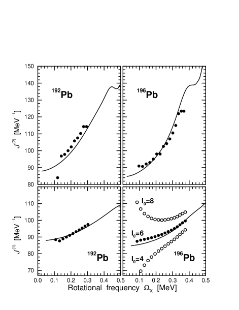
FIG. 2.: The same as in Fig. 1 but for the yrast SD bands in ^192,196Pb. The experimental data are taken from Refs. [33] (¹⁹²Pb) and [35] (¹⁹⁶Pb). The experimental $J^{(1)}$ values of the ¹⁹²Pb band are shown for the spin value of $I_{0}=8$ for the lowest state in the SD band (the lowest transition with the energy 214.8 keV corresponds to a spin change $10\rightarrow 8$). The experimental $J^{(1)}$ values of the ¹⁹⁶Pb band are shown for three different values of $I_{0}$. The values being in best agreement with calculations are indicated by solid circles.

The present calculations have been performed with the NL1 parametrization [32] of the relativistic mean field Lagrangian. The CRHB-equations are solved in the basis of an anisotropic three-dimensional harmonic oscillator in Cartesian coordinates. A basis deformation of $\beta_{0}=0.5$ has been used. All fermionic and bosonic states belonging to the shells up to $N_{F}=14$ and $N_{B}=16$ are taken into account in the diagonalisation and the matrix inversion, respectively. This truncation scheme provides reasonable numerical accuracy. For example, the increase of the fermionic basis up to $N_{F}=17$ changes the values of the kinematic moment of inertia $J^{(1)}$ and the transition quadrupole moment $Q_{t}$ by less than 1%. The numerical errors for the total energy are even smaller.

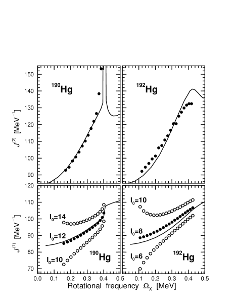
FIG. 3.: The same as in Fig. 2 but for the yrast SD bands in ^190,192Hg. The experimental data are taken from Refs. [36] (¹⁹⁰Hg) and [37] (¹⁹²Hg).

Yrast SD bands in ¹⁹⁴Pb and ¹⁹⁴Hg are linked to the low-spin level scheme [28, 29, 31]. In addition, there is a tentative linking of SD band in ¹⁹²Pb [33]. These data provide an opportunity to compare with experiment in a direct way not only calculated dynamic ($J^{(2)}$) but also kinematic ($J^{(1)}$) moments of inertia. On the contrary, at present the yrast SD bands in ^190,192Hg and ¹⁹⁶Pb are not linked to the low-spin level scheme yet. Thus some spin values consistent with the signature of the calculated yrast SD configuration should be assumed for the experimental bands when a comparison is made with respect of the kinematic moment of inertia $J^{(1)}$.

The results of such a comparison are shown in Figs. 1, 2 and 3. The theoretical $J^{(1)}$ values agree well with the experimental ones in the cases of linked SD bands in ¹⁹⁴Pb and ¹⁹⁴Hg and tentatively linked SD band in ¹⁹²Pb. The comparison of theoretical and experimental $J^{(1)}$ values (see Figs.  2 and 3) indicates that the lowest transitions in the yrast SD bands of ¹⁹⁰Hg, ¹⁹²Hg and ¹⁹⁶Pb with energies 316.9, 214.4 and 171.5 keV, respectively, most likely correspond to the spin changes of $14^{+}\rightarrow 12^{+}$, $10^{+}\rightarrow 8^{+}$ and $8^{+}\rightarrow 6^{+}$. If these spin values are assumed, good agreement between theory and experiment is observed. Calculated and experimental values of the dynamic moment of inertia $J^{(2)}$ agree also well, see Figs. 1, 2 and 3.

The increase of kinematic and dynamic moments of inertia in this mass region can be understood in the framework of CRHB theory as emerging predominantly from a combination of three effects: the gradual alignment of a pair of $j_{15/2}$ neutrons, the alignment of a pair of $i_{13/2}$ protons at a somewhat higher frequency, and decreasing pairing correlations with increasing rotational frequency. The interplay of alignments of neutron and proton pairs is more clearly seen in Pb isotopes where the calculated $J^{(2)}$ values show either a small peak (for example, at $\Omega_{x}\sim 0.45$ MeV in ¹⁹²Pb, see Fig. 2) or a plateau (at $\Omega_{x}\sim 0.4$ MeV in ¹⁹⁶Pb, see Fig. 2). With increasing rotational frequency, the $J^{(2)}$ values determined by the alignment in the neutron subsystem decrease but this process is compensated by the increase of $J^{(2)}$ due to the alignment of the $i_{13/2}$ proton pair. This leads to the increase of the total $J^{(2)}$-value at $\Omega_{x}\geq 0.45$ MeV. The shape of the peak (plateau) in $J^{(2)}$ is determined by a delicate balance between alignments in the proton and neutron subsystems which depends on deformation, rotational frequency and Fermi energy. For example, no increase in the total dynamic moment of inertia $J^{(2)}$ has been found in the calculations after the peak up to $\Omega_{x}=0.5$ MeV in ¹⁹²Hg, see Fig. 3. It is also of interest to mention that the sharp increase in $J^{(2)}$ of the yrast SD band in ¹⁹⁰Hg is also reproduced in the present calculations. One should note that the calculations slightly overestimate the magnitude of $J^{(2)}$ at the highest observed frequencies. The possible reasons could be the deficiencies either of the Lipkin-Nogami method [34] or the cranking model in the band crossing region or both of them.

The comparison between calculated and experimental absolute transition quadrupole moments $Q_{t}$ is less straightforward. This is because the uncertainties in absolute measured $Q_{t}$ values arising from the uncertainties in stopping powers can be as large as 15% [38]. Thus the comparison of $Q_{t}$’s values obtained in different experiments should be performed with some caution since systematic errors due to different stopping powers may be responsible for the observed differences. In addition, as illustrated in Fig. 4, the experimental $Q_{t}$ values depend somewhat on the type of analysis (centroid shift or line shape) used when these quantities are extracted from the data.

The results of CRHB calculations are compared with most recent experimental data in Fig. 4. One can conclude that the results of calculations for absolute values of $Q_{t}$ will be within the ‘full’ error bars if the 15% uncertainty due to stopping powers would be taken into account (experimental data shown in Fig. 4 does not include these uncertainties). For the sake of simplicity we will not take into account these uncertainties in the subsequent discussion and will concentrate mainly on the experimental data obtained with the same stopping powers. In Fig. 4 such data are indicated by the same capital letters. While the calculated $Q_{t}$ values are close to the experimental values obtained with centroid shift and line shape analysis for Pb isotopes, most of experimental $Q_{t}$ values (with exception of exp. B) are overestimated in calculations in the case of Hg isotopes. One should note that the most recent experimental data on ¹⁹²Hg is contradictory since two experiments (exp. A [38] and exp. B [39]) give very different values of $Q_{t}$, see Fig. 4. Definitely, the measurements of relative transition quadrupole moments between SD bands in Pb and Hg isotopes using the same stopping powers, which are not available nowadays, are needed to find out, whether this discrepancy between calculations and experiment is due to an inadequate theoretical description or the experimental problems quoted above. In the calculations, relative average quadrupole moments $\Delta Q_{t}$ between yrast SD bands of Pb and Hg isotopes decrease with increasing neutron number $N$ ($\Delta Q_{t}\approx 1.6$ $e$b, $\approx 1.4$ $e$b and $\approx 1.06$ $e$b for $N=110,112$ and 114, see Fig. 4).

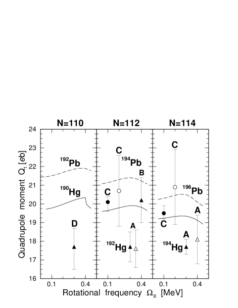
FIG. 4.: Measured and calculated transition quadrupole moments $Q_{t}$ of the yrast SD bands. Solid and dashed lines show the results of calculations for Hg and Pb isotopes, respectively. Experimental values are given by error bars where the type of symbols corresponding to experimental middle value of $Q_{t}$ indicates the isotope and type of analysis used to extract the experimental value. The following correspondence exists: circles - Pb isotopes, triangles - Hg isotopes, open symbols - line shape analysis, filled symbols - centroid shift. The experimental data are taken from Refs. [38] (exp. A), [39] (exp. B), [40] (exp. C), and [41] (exp. D). Experimental data on ¹⁹²Pb are not available.

Results of calculations indicate the general trend of decrease of average $Q_{t}$ values with the increase of neutron number $N$ both for Pb and Hg isotopes. The results of the centroid shift analysis for ^194,196Pb (exp. C) indicate a slight decrease in the $Q_{t}$ values with increasing $N$ consistent with theoretical results. Although the data on ^192,194Hg (exp. A) indicate similar values of $Q_{t}$ being in slight contradiction with theoretical results, definite conclusions are not possible at present due to the large error bars. In addition, with increasing rotational frequency $\Omega_{x}$ the calculated $Q_{t}$ values show initially a slight increase which is followed by a subsequent decrease. In the case of ¹⁹⁰Hg this feature is hidden by the band crossing. The maximum $Q_{t}$ values within specific configurations are calculated at different frequencies $\Omega_{x}$ as a function of the neutron number $N$. With increasing $N$ the maximum $Q_{t}$ is reached at lower frequencies. Similar variations of $Q_{t}$ have been also observed in the cranked Hartree-Fock calculations with Skyrme forces [13]. Dedicated experiments aiming on the measurements of the variations of transition quadrupole moments $Q_{t}$ as a function of rotational frequency $\Omega_{x}$ are needed in order to confirm or reject these results.

In conclusion, the Cranked Relativistic Hartree-Bogoliubov theory has been developed and applied to the description of yrast SD bands observed in the $A\sim 190$ mass region. With an approximate particle number projection performed by the Lipkin-Nogami method, the rotational features of experimental bands such as kinematic and dynamic moments of inertia are very well described in the calculations. Calculated values of transition quadrupole moments $Q_{t}$ are close to the measured ones, however, more accurate and consistent experimental data on $Q_{t}$ is needed in order to make detailed comparisons between experiment and theory.

A.V.A. acknowledges support from the Alexander von Humboldt Foundation. This work is also supported in part by the Bundesministerium für Bildung und Forschung under the project 06 TM 875.

REFERENCES

- [1] Permanent address: Nuclear Research Center, Latvian Academy of Sciences, LV-2169 Salaspils, Latvia.
- [2] C. E. Svensson et al., Phys. Rev. Lett. 82, 3400 (1999).
- [3] B. Singh, R. B. Firestone, and S. Y. F. Chu, Nuclear Data Sheets 78, 1 (1996).
- [4] W. Koepf and P. Ring, Nucl. Phys. A493, 61 (1989); Nucl. Phys. A511, 279 (1990).
- [5] J. König and P. Ring, Phys. Rev. Lett. 71, 3079 (1993).
- [6] A. V. Afanasjev, J. König, and P. Ring, Nucl. Phys. A608, 107 (1996).
- [7] A. V. Afanasjev, G. A. Lalazissis, and P. Ring, Acta Phys. Hung. 6, 299 (1997).
- [8] A. V. Afanasjev, G. A. Lalazissis, and P. Ring, Nucl. Phys. A634, 395 (1998).
- [9] A. V. Afanasjev, I. Ragnarsson, and P. Ring, Phys. Rev. C 59, 3166 (1999).
- [10] M. Devlin et al., Phys. Rev. Lett. 82, 5217 (1996).
- [11] W. Satuła, S. Ćwiok, W. Nazarewicz, R. Wyss, and A. Johnson, Nucl. Phys. A529, 289 (1991).
- [12] W. Satuła, and R. Wyss, Phys. Rev. C 50, 2888 (1994).
- [13] J. Terasaki, P.-H. Heenen, P. Bonche, J. Dobaczewski, and H. Flocard, Nucl. Phys. A593, 1 (1995).
- [14] B. Gall, P. Bonche, J. Dobaczewski, H. Flocard, and P.-H. Heenen, Z. Phys. A 348, 183 (1994).
- [15] M. Girod, J. P. Delaroche, J. F. Berger, and J. Libert, Phys. Lett. B 325, 1 (1994).
- [16] A. Valor, J. L. Egido, and L. M. Robledo, Phys. Lett. B 392, 249 (1997).
- [17] W. Satuła, R. Wyss, and P. Magierski, Nucl. Phys. A578, 45 (1994).
- [18] H. J. Lipkin, Ann. Phys. 31, 525 (1960).
- [19] Y. Nogami, Phys. Rev. 134, 313 (1964).
- [20] H. C. Pradhan, Y. Nogami, and J. Law, Nucl. Phys. A201, 357 (1973).
- [21] Y. Sun, Jing-ye Zhang, and M. Guidry, Phys. Rev. Lett. 78, 2321 (1997).
- [22] B. D. Serot, and J. D. Walecka, Adv. Nucl. Phys. 16, 1 (1986).
- [23] J. F. Berger, M. Girod, and D. Gogny, Comp. Phys. Comm. 63, 365 (1991).
- [24] W. Pöschl, D. Vretenar, G. A. Lalazissis, and P. Ring, Phys. Rev. Lett. 79, 3841 (1997).
- [25] D. Vretenar, G. A. Lalazissis, and P. Ring, Phys. Rev. Lett. 82, 4595 (1999).
- [26] G. A. Lalazissis, D. Vretenar, and P. Ring, Phys. Rev. C 57, 2294 (1998).
- [27] B. J. P. Gall et al., Phys. Lett. B 345, 124 (1995).
- [28] A. Lopez-Martens et al., Phys. Lett. B 380, 18 (1996).
- [29] K. Hauschild et al., Phys. Rev. C 55, 2819 (1997).
- [30] B. Cederwall et al., Phys. Rev. Lett. 72, 3150 (1994).
- [31] T. L. Khoo et al., Phys. Rev. Lett. 76, 1583 (1996).
- [32] P.-G. Reinhard, M. Rufa, J. Maruhn, W. Greiner, and J. Friedrich, Z. Phys. A 323, 13 (1986).
- [33] D. P. McNabb et al., Phys. Rev. C 56, 2474 (1997).
- [34] P. Magierski, S. Ćwiok, J. Dobaczewski, and W. Nazarewicz, Phys. Rev. C 48, 1686 (1993).
- [35] U. J. van Severen et al., Z. Phys. A 353, 15 (1995).
- [36] A. N. Wilson et al., Phys. Rev. C 54, 559 (1996)
- [37] P. Fallon et al., Phys. Rev. C 51, R1609 (1995)
- [38] E. F. Moore et al., Phys. Rev. C 55, R2150 (1997).
- [39] B. C. Busse et al., Phys. Rev. C 57, R1017 (1998).
- [40] U. J. van Severen et al., Phys. Lett. B 434, 14 (1998).
- [41] H. Amro et al., Phys. Lett. B 413, 15 (1997).