Reconstructing the Freeze-out State in Pb+Pb Collisions at 158 $A$GeV/$c$

Abstract

For a class of analytical parametrizations of the freeze-out state of relativistic heavy ion collisions, we perform a simultaneous analysis of the single-particle $m_{\perp}$-spectra and two-particle Bose-Einstein correlations measured in central Pb+Pb collisions at the CERN SPS. The analysis includes a full model parameter scan with $\chi^{2}$ confidence levels. A comparison of different transverse density profiles for the particle emission region allows for a quantitative discussion of possible model dependencies of the results. Our fit results suggest a low thermal freeze-out temperature $T\approx 95\pm 15\,\mbox{MeV}$ and a large average transverse flow velocity $\bar{v}_{\perp}\approx 0.55\pm 0.07$. Moreover, the fit favours a box-shaped transverse density profile over a Gaussian one. We discuss the origins and the consequences of these results in detail. In order to reproduce the measured pion multiplicity our model requires a positive pion chemical potential. A study of the pion phase-space density indicates $\mu_{\pi}\approx 60\,\mbox{MeV}$ for $T=100\,\mbox{MeV}$.

I Introduction

The space-time analysis of hadronic one- and two-particle spectra measured in relativistic heavy ion collisions has attracted much attention in recent years. Via the reconstruction of the hadronic phase-space distribution at freeze-out, this method can provide detailed geometrical and dynamical information about the last stage of the collision. The ultimate goal of the experimental relativistic heavy ion program is to produce and test the dense early stage of the collision in which quarks and gluons are the relevant degrees of freedom and a quark-gluon-plasma is expected (for an up-to-date overview see [1, 2]). However, only the hadronized remnants of this state are experimentally accessible. Characterizing their spatial and dynamical distribution, a particle interferometry based space-time analysis can provide estimates of the phase-space density attained in the collision and it can establish an experimentally determined endpoint for microscopic simulations of the complicated multiparticle dynamics. This makes it a valuable tool in the search for the quark-gluon-plasma.

One of the main motivations for space-time analyses in recent years is the discovery that HBT (Hanbury Brown and Twiss) particle interferometry allows to disentangle between random and directed dynamical components in the collision [3, 4, 5, 6, 7, 8]. Specifically, in the context of hydrodynamic parametrizations which provide a very convenient characterization of the freeze-out region, the one-particle spectra are determined by an effective blue-shifted temperature from which temperature and flow effects cannot be separated unambiguously [9]. On the other hand, the $M_{\perp}$-dependence of the transverse correlation radii increases with transverse flow but decreases with stronger thermal smearing [10]. By combining both observables the ambiguity between temperature and flow can be removed.

Knowledge of the magnitude of the transverse flow is crucial for a dynamical picture of the transverse expansion of the collision system and for a dynamical back-extrapolation into the hot and dense early stage of the collision. With this motivation, there have been several recent discussions about disentangling temperature and flow effects. Except for the recent analysis in [11] most of these discussions are published in conference proceedings and reviews [7, 8, 12, 13, 14], and they are mainly based on preliminary data. None of them provides a full model parameter scan with $\chi^{2}$ confidence levels for the two-particle spectra, and none of them makes quantitative statements about the model-dependence of the conclusions reached. However, both these points are very important, since one may wonder, e.g., to what extent the main conclusions, a relatively low temperature and high transverse flow velocity, are subject to model-dependent details of the parametrization. The present work addresses this gap in the literature with an extensive model study.

Three collaborations measured and published data on Bose-Einstein correlations for 158 $A$GeV/$c$ Pb+Pb collisions at the CERN SPS: WA98 [15], NA44 [16] and NA49 [11]. Due to their small acceptance, NA44 can only determine particle correlations in two transverse momentum bins which moreover correspond to slightly different rapidities. Such data are not well suited for a detailed analysis where the $M_{\perp}$-dependence of the correlation radii plays a crucial role. The situation is somewhat better for the recently presented WA98 data [15] but these were not yet available at the time of the present analysis. Most suited for our analysis tool is a large acceptance experiment like NA49 which covers almost the whole forward rapidity region. Their published data are, however, given only in the YKP parametrization [11]. Although in many situations its parameters have the most straightforward physical interpretation [17], this parametrization can be ill-defined in some kinematic regions [18, 19], and a cross-check with Cartesian (Pratt-Bertsch) correlation radii is hence necessary. The NA49 experiment has the unique capability of cross-checking experimental results from different detector components with overlapping acceptance. At the moment, the remaining differences between the different detectors are still larger than the published error bars [20]. We address these subtleties in Section II where we discuss in detail the data used in our analysis.

The class of fireball models used for our analysis was described in detail elsewhere (for recent reviews see e.g. [12, 13]). To get an idea of the degree of model dependence of our final conclusions we here investigate two different transverse density distributions, a box-shaped and a Gaussian profile. The relevant model parameters are shortly introduced in Section III. Up to now our analysis is restricted to the transverse momentum dependence in the particular rapidity bin ($3.9<Y<4.4$) for which a complete set of HBT parameters was published in [11]. A realistic description of the rapidity dependence of the transverse one-particle spectra would require a refined model [5, 21, 22]. The results of the fit, as well as related technical details, are given in Section IV.

As an application of these results we discuss in Section V the average pion phase-space density at freeze-out. Bertsch [23] pointed out that knowledge of the single-particle spectrum and Bose-Einstein correlations allows for a model-independent extraction of this quantity. The reason is that absolutely normalized single-particle spectra carry information about the particle density in momentum space while the width of the distribution in configuration space can be extracted from correlation studies. We extract this model-independent quantity from the data and compare it with the prediction of our model; in this way we determine the value of the pion chemical potential needed to reproduce the measured pion yields. This is an interesting quantity since a large value of $\mu_{\pi}$ would indicate an “overpopulation” of phase-space and could indicate the onset of multiparticle effects (e.g. stimulated emission or a pion laser).

Section VI contains our conclusions. Technical details are deferred to three Appendices.

II The data

Data on the Bose-Einstein correlation radii as functions of $K_{\perp}$ from the 5% most central Pb+Pb collisions at 158 $A$ GeV/$c$ were published by the NA49 collaboration [11] for the rapidity window $Y\in(3.9,\,4.4)$ (i.e. $1\leq Y_{{}_{\rm CM}}\leq 1.5$). Our analysis will focus on these data.

The single-particle $p_{\perp}$-distributions of negatively charged hadrons ($h^{-}$) are taken from [24]. At the time of our analysis, spectra of identified pions were not yet available for the above rapidity window. The differences between $h^{-}$ and identified pion spectra (from negative kaons and a few antiprotons) are, however, small since most negatively charged hadrons are pions. This is good since these differences will have to be modelled and thus introduce (small) systematic uncertainties. The rapidity binning of the $h^{-}$ data in [24] is slightly different from that of the correlation analysis of [11]. For $h^{-}$ we use the bin $4.15<y<4.65$ which has the largest overlap with that of the correlation data. This is an excellent approximation since the $p_{\perp}$-spectra vary only weakly with rapidity in this region [24].

For wide bins the question arises where exactly the data points should be placed when comparing them to model predictions. Usually one puts them in the middle of the bins. This may, however, lead to systematic errors [25] if the measured distribution is not flat. Our procedure “where to stick the data point” is state of the art [25]: if the measured distribution is well parameterized by a function $g(x)$, then the appropriate position of the data point corresponding to a bin of width $\Delta x$ between $x_{1}$ and $x_{2}$ is obtained as

$$x^{\rm bin}=g^{-1}\left(\frac{1}{\Delta x}\int_{x_{1}}^{x_{2}}g(x)\,dx\right)\,,$$ (1)

where $g^{-1}$ is the inverse function of $g$. The position of the data points of the single-particle spectrum in rapidity is calculated from this equation using for $g(x)$ the distribution (A1) with $\Delta y=1.4$ [26, 27]; to get the appropriate positions in transverse momentum, the parametrization (A5) with $T_{\rm inv}=185\,\mbox{MeV}$ (inferred from the measured average transverse momentum and the fact that the observed $p_{\perp}$-spectrum is very well parameterized by an exponential with inverse slope $T_{\rm inv}$) is used for $g(x)$. Note that the width of the $p_{\perp}$ bins in the used data was 100 MeV/$c$, with the first bin starting at 50 MeV/$c$. For these data we have explicitly checked that taking the data points in the centres of the bins or according to the above described procedure does not lead to an observable difference in the fit results.

The HBT two-particle correlation radii published in [11] for the rapidity window $1\leq Y_{{}_{\rm CM}}\leq 1.5$ have several shortcomings which can only be resolved in future experimental analyses: First, the correlation radii are only given for the YKP parametrization. Their statistical uncertainties are systematically larger than for the Cartesian parametrization [28, 29], and the data shown in [11] do not allow for the important cross-check [17, 18, 19] with the Cartesian parameterization. This is an important issue since the YKP fit was recently found to be problematic [18, 19]. Second, Ref. [11] contains only data taken in the Main Time Projection Chamber (MTPC), in spite of the observed systematic differences between radii extracted from the MTPC [28] and the VTPC data [29] (of the order of 0.5 fm [20]). The error bars in [11] do not include this systematic uncertainty which is only roughly estimated to be about 15%.

To address these difficulties we based our analysis on the three accessible, but so far unpublished complete data sets from the NA49 experiment: $h^{+}h^{+}$ and $h^{-}h^{-}$ correlations from the VTPC [29] and $h^{-}h^{-}$ correlations from the MTPC [28]. The reported errors are the output of the MINUIT fitting routine which is known to underestimate errors [30]. For our analysis we considered these three data sets as independent measurements and took their average, with correspondingly increased error bars which now also include the systematic deviations between these measurement. Since both in theory and experiment the squared correlation radii and the YK velocity are the directly determined fit parameters [17, 31], we average over and fit to those.

The obtained fit parameters for the Cartesian and YKP parametrizations are summarized in Tables I and II, respectively. They are also displayed in Figs. 1 and 2. The minor difference between the rapidity bins of the VTPC analysis [29] ($3.9<Y<4.4$) and the MTPC analysis [28] ($4<Y<4.5$) is irrelevant and has been neglected. The binning in transverse momentum differs slightly, too. Only four of the total number of five $K_{\perp}$ bins could be taken into account in the averaging procedure, and for the fourth bin a slight size difference between [28] and [29] (see Table I) had to be neglected. To position the data points in the bins we assumed here that their distribution $g(x)$ inside the bin can be linearized. Then their position in the bin $[x_{1},x_{2}]$ can be calculated from [25]

$$x^{\rm bin}=\frac{\int_{x_{1}}^{x_{2}}x\,g(x)\,dx}{\int_{x_{1}}^{x_{2}}g(x)\,dx}\,.$$ (2)

Inserting for the function $g(x)$ the distribution $\varrho_{2}^{Y}(Y)$ from equation (A3) with $\Delta y=1.4$ into (2), the position of the data points in the pair rapidity $Y$ is obtained: $Y^{\rm bin}_{{}_{\rm CM}}=1.22$. The values of $K_{\perp}^{\rm bin}$ for the different $K_{\perp}$-bins are calculated using for $g(x)$ the function $\varrho_{2}^{\perp}(K_{\perp})$ from equation (A13), again with $T_{\rm inv}=185\,\mbox{MeV}$. The resulting values are displayed in Tables I and II. We observed [19] that slightly different (worse) model fits are obtained if the data points are placed at the bin centres rather than at the positions calculated from (2).

It remains to check the compatibility of the Cartesian and YKP correlation parameters in order to ascertain the validity of the YKP data. To this end the Cartesian radii were calculated from the YKP parameters and vice versa via cross-check relations published in [17, 18]. The resulting calculated radius parameters are shown in Figs. 1 and 2 by gray dashed symbols. The errors were propagated to the calculated radii via

$$\sigma_{i}=\sqrt{\sum_{j}\left(\frac{\partial R_{i}^{2}}{\partial R_{j}^{\prime 2}}\right)^{2}\,\sigma_{j}^{\prime 2}}\,,$$ (3)

where $\sigma_{i}$ is the calculated error of the Cartesian (YKP) correlation parameter $R_{i}^{2}$ and $\sigma_{j}^{\prime}$ the “measured” error of the YKP (Cartesian) parameter $R_{j}^{\prime 2}$. (Here the notion ‘YKP correlation parameter’ includes radius parameters as well as the YK velocity $v_{{}_{\rm YK}}$.) Note that the non-diagonal terms of the error matrix are not known and had to be neglected. In most cases the calculated parameters show larger errors than the directly measured ones. This might improve if non-diagonal error matrix elements could be taken into account in Eq. (3).

Figs. 1 and 2 show that the YKP and Cartesian data are “on average” consistent [32]. In view of the known fragility of YKP fits this is an important and non-trivial result. However, it was recently argued [18, 19] that the YKP parametrization is quite subtle and can become ill-defined for certain (even realistic) sources. The only way to test this possibility in experiment is to calculate the YKP parameters from the Cartesian ones and check that the resulting values are real. Since experimental Cartesian radius parameters have a finite measurement error, it is not sufficient to perform this consistency check only for their average values; rather, all parameter values within the error interval should be checked. When doing so we found problems with the definition of the YKP parameters inside the error intervals for the third and fourth $K_{\perp}$ bins. These may be related to our further observation [19] that no good model fit was possible starting from the YKP parameters, and that the fits tended to drift into strange parameter regions. This emphasizes the future need for an explicit cross-check between Cartesian and YKP parameter fits directly on the experimental level, including error propagation with the complete error matrix. Due to our problems with the measured YKP parameters, the model fits presented here are based on an analysis of the Cartesian correlation radii.

III The model

A The emission function

Our model analysis is based on the widely used emission function [3, 4, 31, 33, 34, 35]

$$S(x,K)\,d^{4}x = \frac{M_{\perp}\cosh(Y-\eta)}{(2\pi)^{3}}\,\exp\left(-\frac{K\cdot u(x)}{T}+\frac{\mu}{T}\right)$$ (6)

$$\times G(r)\,\exp\left(-\frac{(\eta-\eta_{0})^{2}}{2(\Delta\eta)^{2}}\right)\,d\eta\,r\,dr\,d\varphi$$

$$\times\frac{\tau\,d\tau}{\sqrt{2\pi(\Delta\tau)^{2}}}\,\exp\left(-\frac{(\tau-\tau_{0})^{2}}{2(\Delta\tau)^{2}}\right)\,.$$

Here, the pair momentum $K$ is parameterized in terms of the transverse mass $M_{\perp}=\sqrt{K_{\perp}^{2}+m^{2}}$, longitudinal rapidity $Y$, and the transverse momentum $K_{\perp}$

$$K=(M_{\perp}\cosh Y,\,K_{\perp},\,0,\,M_{\perp}\sinh Y)\,.$$ (7)

We use here the usual coordinate system with x-axis directed parallel to $\leavevmode\text{tensysevensyfivesy\boldmath{$K$}}_{\perp}$. In configuration space, we use the polar coordinates $r$ and $\varphi$ for the transverse directions, a longitudinal proper time $\tau=\sqrt{t^{2}-z^{2}}$ and space-time rapidity $\eta=\frac{1}{2}\ln\frac{t+z}{t-z}$.

The $\eta$-profile in the model is chosen to be a Gaussian peaked at $\eta_{0}$ with width $\Delta\eta$. In this way $\eta_{0}$ determines the centre of mass (CMS) rapidity. Since we focus on a single rapidity bin and work in the LCMS, we set $\eta_{0}=-1.22$ (see previous Section) and $\Delta\eta=1.3$. The latter value is obtained from a comparison with the single-particle rapidity distribution.

Freeze-out proper times are distributed according to a Gaussian of width $\Delta\tau$ centred at $\tau_{0}$. This allows for freeze-out of particles during an extended time period given by $\Delta\tau$.

The transverse geometry is specified by the distribution $G(r)$ in (6). As only azimuthally symmetric fireballs are considered, this function does not depend on $\varphi$. In our analysis two particular profiles will be assumed: a Gaussian one

$$G(r)=\exp\left(-\frac{r^{2}}{2R_{G}^{2}}\right)\,,$$ (8)

and a box-shaped one

$$G(r)=\theta(R_{B}-r)\,.$$ (9)

The fireball at freeze-out is assumed to be in local thermal equilibrium at temperature $T$. This is modelled by the Boltzmann factor in (6). The chemical potential $\mu$ in its argument has no effect on the correlation radii and only affects the normalization of the single particle spectrum. The argument $K{\cdot}u(x)$ allows for longitudinal and transverse expansion of the fireball through the collective four-velocity field $u(x)$:

$$u(x) = \left(\cosh\eta_{t}\,\cosh\eta,\,\cos\varphi\,\sinh\eta_{t},\,\sin\varphi\,\sinh\eta_{t},\right.$$ (11)

$$\left.\qquad\qquad\qquad\cosh\eta_{t}\,\sinh\eta\right)\,.$$

The longitudinal expansion rapidity $\eta_{l}(x)$ has here been identified with the space-time rapidity $\eta$. This leads to a longitudinal expansion velocity $v_{\rm long}(z,t)=\tanh\eta=z/t$, corresponding to Bjorken-type boost-invariant expansion [36]. The transverse expansion is parameterized by the transverse flow rapidity $\eta_{t}(x)$. It is assumed to increase linearly with the distance from the collision axis,

$$\eta_{t}(x)=\eta_{f}\frac{r}{r_{\rm rms}}\,.$$ (12)

The scaling factor $\eta_{f}$ specifies the value of the transverse flow rapidity at the transverse rms radius, given by

$$r_{\rm rms}=\sqrt{2}R_{G}$$ (13)

for the Gaussian transverse distribution and by

$$r_{\rm rms}=\frac{R_{B}}{\sqrt{2}}$$ (14)

for the box-shaped one. From these relations we expect the two fit parameters in (8) and (9) to satisfy approximately $R_{B}\approx 2\,R_{G}$.

In the literature the transverse flow is often quoted in terms of the average transverse expansion velocity $\bar{v}_{\perp}$

$$\bar{v}_{\perp}=\frac{\int_{0}^{\infty}r\,dr\,\tanh\eta_{t}(r)\,G(r)}{\int_{0}^{\infty}r\,dr\,G(r)}\,.$$ (15)

Its value is roughly given by the radial velocity at the transverse rms radius, $v_{\perp}(r_{\rm rms})\simeq\tanh\eta_{f}$; looking more closely, it is slightly smaller: for $\eta_{f}$=0.6 one finds $v_{\perp}(r_{\rm rms}){\approx}0.54$ and $\bar{v}_{\perp}$=0.50 (0.46) for the box-like (Gaussian) transverse density profile.

Our calculation of the single-particle spectra from (6) includes contributions from resonance decays as described in [9, 37]. This is crucial for a correct description of the yield and shape of the spectra. We include all decays with branching ratios above 1% from mesons with masses up to 1020 MeV/$c^{2}$ and from baryons with masses up to 1400 MeV/$c^{2}$. For decay chains, the product of the branching ratios is required to be larger than 1%. For baryons the chemical potential $\mu_{B}(T)$ was parameterized according to (B1). Strange particles acquire a chemical potential $\mu_{S}(T)$ determined by the condition (B2) of strangeness neutrality. Finally, contributions from negative kaons and antiprotons were included in the calculation of the $h^{-}$ spectrum.

The role of resonance decay contributions to the HBT radius parameters is known to be much less important [37]. Our calculation of the correlation radii will thus only include direct pions. This is an essential technical simplification: the additional integrals from the resonance decay phase space would have increased the numerical task from calculating a 2-dimensional integral to calculating a 5-dimensional (for two-particle decays) or 6-dimensional one (for three-particle decays). This very time consuming calculation was performed in model studies [37] where the correlator was evaluated for only a few characteristic sets of model parameters. However, in a simultaneous multi-parameter fit, in which the fit routine calls the two-particle correlator approximately 50-100 times for thousands of different model parameter combinations, it cannot be done.

We finally remark that the model (6) is customarily used with a Boltzmann distribution rather than a Bose-Einstein one, since this greatly simplifies the analytical and numerical analysis. The resulting differences are usually small. If the pions develop a positive chemical potential, however, this visibly affects the shape of the single particle spectra; for this reason we use, in fact, a Bose-Einstein distribution to calculate the pion multiplicities and the single-particle spectra of direct pions (see Appendix B and C). For the heavier resonances the Boltzmann approximation is excellent. For technical reasons we also use the Boltzmann approximation in the calculation of the correlation radii, in line with the much larger systematic error of the corresponding available data.

B Basic relations

We shortly recall how the emission function $S(x,K)$ is related with the observables to be calculated. More details can be found e.g. in [12].

The single-particle spectrum is obtained from

$$E_{p}\frac{dN}{d^{3}p}=P_{1}(p)=\int d^{4}x\,S(x,p)\,.$$ (16)

For the two-particle correlations, we used the Cartesian parametrization:

$$C(q,K)-1 = \exp\left[-q_{o}^{2}R_{o}^{2}(K)-q_{s}^{2}R_{s}^{2}(K)\right.$$ (18)

$$\qquad\left.-q_{l}^{2}R_{l}^{2}(K)-2q_{o}q_{l}R_{ol}^{2}(K)\right]\,,$$

where the $q_{i}$ are the components of the momentum difference in the out-side-long coordinate system and $K$ stands for the average pair momentum. The correlation radii are obtained from the emission function via

$$R_{s}^{2} = \langle\tilde{y}^{2}\rangle\,,$$ (20)

$$R_{o}^{2} = \langle(\tilde{x}-\beta_{\perp}\tilde{t})^{2}\rangle\,,$$ (21)

$$R_{l}^{2} = \langle(\tilde{z}-\beta_{l}\tilde{t})^{2}\rangle\,,$$ (22)

$$R_{ol}^{2} = \langle(\tilde{x}-\beta_{\perp}\tilde{t})(\tilde{z}-\beta_{l}\tilde{t})\rangle\,.$$ (23)

Here

$$\tilde{x}_{\mu}=x_{\mu}-\bar{x}_{\mu}\,,\qquad\bar{x}_{\mu}(K)=\langle x_{\mu}\rangle\,,$$ (24)

and

$$\langle f(x)\rangle(K)=\frac{\int d^{4}x\,f(x)\,S(x,K)}{\int d^{4}x\ S(x,K)}\,.$$ (25)

In our calculations all integrations were performed numerically. This distinguishes our work from Ref. [14] where analytic approximations were used instead. For sources with strong transverse flow (as will be the case here) the analytical approximations for the correlation radii may become problematic [33, 34, 38]. Also, it is not easy to capture the intricate effects of resonance decay kinematics on the single-particle spectra with simple analytical expressions as those used in [14].

IV The Fit

A Single-particle $p_{\perp}$-spectrum

The first step is to fit the $h^{-}$ single-particle $p_{\perp}$-spectrum with the model (6). Resonance decay contributions are treated as described in Sec. III A. The geometrical model parameters $\Delta\eta$, $R_{B}$ ($R_{G}$), $\tau_{0}$, $\Delta\tau$ are known to only affect the absolute normalization of the single-particle spectrum, but not its shape [9, 12]. For fixed transverse density and flow profiles, the spectral shape is completely determined by the temperature $T$ and the transverse flow strength $\eta_{f}$.

The fit to the spectrum was performed with the CERN package MINUIT [39], using for the calculation of (16) (see Appendix B) a routine described in [37]. The data were compared with the $y$-integrated $m_{\perp}$-spectrum rather than with the spectrum at a fixed value of $y$. Since the $y$-integration can be done analytically and removes the dependence on the longitudinal kinematic limits for resonance decays, the former requires much less computation time. The differences are very small since the $m_{\perp}$-spectra obtained from (6) are almost $y$-independent, except for very forward/backward rapidities.

The resulting $\chi^{2}$ contour plots in $T$ and $\eta_{f}$ are shown in Figs. 3 (box-shaped transverse geometric profile) and 4 (Gaussian profile). For comparison the average transverse expansion velocity $\bar{v}_{\perp}$ is given on the right ordinates of these Figures. For their calculation the routine was driven through the whole $T$-$\eta_{f}$ domain covered by the Figures, and in each point the normalization of the spectrum was fitted as a third parameter. One finds a clear $\chi^{2}$ “valley” pointing from the upper left to the lower right corner, reflecting the anticorrelation between $T$ and $\eta_{f}$ in the $m_{\perp}$-slope. The indicated confidence levels result from a $\chi^{2}$-distribution with 16 degrees of freedom (19 data points minus 3 fit parameters) [40].

The two panels of Fig. 3 show the effects of including the $K^{-}$ and $\bar{p}$ contributions in the negative hadron spectra – the upper panel includes only negative pions (including all resonance decays). At low temperature the fit results are nearly identical because the $K^{-}$ and $\bar{p}$ contributions are strongly suppressed by their masses and by the large baryon chemical potential (at $T$=80 MeV we have $\mu_{B}\approx 430$ MeV), but at higher temperatures their inclusion reduces appreciably the amount of transverse flow needed to fit the measured slope. Our results differ in two points from those published in [7]: (i) We include nonzero baryon and strangeness chemical potentials. This increases the decay contributions from baryon resonances, making the spectra steeper and thus requiring more transverse flow to reproduce the measured slope. Compared to the case of vanishing chemical potentials this shifts the “$\chi^{2}$ valley” in Fig. 3a upwards by $\approx$ 0.05 $c$ (somewhat less at low $T$ and more for higher $T$). (ii) We include contributions from $K^{-}$ and $\bar{p}$. This flattens the $h^{-}$-spectrum further because these heavier particles are more strongly affected by transverse flow. To fit a given spectral slope, lower values of $\eta_{f}$ are thus needed at given $T$. The two effects (i) and (ii) are seen to partially cancel each other.

A comparison of Figs. 3 and 4 gives a feeling for the model-dependence of the fit resulting from two different choices for the transverse density profile. Since at fixed $\eta_{f}$ they lead to different average transverse flow velocities $\bar{v}_{\perp}$ (the quantity which determines the blueshift of the spectral slope), one should use the labelling on the r.h.s. of these Figures for comparison. One sees that for a Gaussian density profile slightly smaller values for $\bar{v}_{\perp}$ are needed to account for the measured slope. The reason is that superimposing a Gaussian distribution $G(r)$ with a monotonically increasing transverse flow profile, a significant part of the high-$p_{\perp}$ part of the spectrum is obtained from contributions at large transverse distances $r>R_{G}$ in the Gaussian tails. A box profile does not allow for emission from distances $r>R_{B}$ and thus requires slightly larger values for $\bar{v}_{\perp}$ to account for the same spectra.

Some access to the shape of the transverse density profile is possible through two-particle correlations (see Sec. IV B), but limited statistics and other uncertainties leave some room for interpretation. The differences between Figs. 3 and 4 should thus be mainly taken as an estimate for the systematic model uncertainties in the finally extracted values for $T$ and $\bar{v}_{\perp}$. That they are small for the single-particle fits is certainly gratifying.

B Two-particle correlations

The correlation radii summarized in Table I were fitted with the CERN package MINUIT [39], using for the model calculation a routine which computes the correlation radii from (III B). We scanned the whole $T$-$\eta_{f}$ domain as before, performing in each point a 3-parameter fit to find the best values of $R_{B}$ ($R_{G}$), $\tau_{0}$, and $\Delta\tau$. $\Delta\eta=1.3$ was always kept fixed, see Sec. III.

The results of these fits, superimposed on the fit of the single-particle spectra, are shown in Figs. 5 (box-profile) and 6 (Gaussian profile). The contours correspond to a $\chi^{2}$-distribution of 11 degrees of freedom (16 data points minus 5 model parameters). These results will be further discussed in Sec. IV D. Here we only observe that the HBT radii indeed allow to disentangle the ambiguity between temperature and transverse flow (although the uncertainties are still significant). The box-shaped transverse geometric profile seems to be favoured by the fit, although limited statistics does not allow to rule out a Gaussian shape. Independent of the choice of the transverse density profile we can, however, safely conclude that the data require strong transverse flow with $\bar{v}_{\perp}>0.3$. The best fits favour low freeze-out temperatures between 80 and 110 MeV and large average transverse expansion velocities between 0.47 $c$ to 0.62 $c$ (for the box model).

On the other hand, the “$\chi^{2}$ valley” defined by the correlation radii is clearly seen to deviate from the simple dependence on $\eta_{f}$ and $T$ which one obtains in analytical approximation for Gaussian transverse density profiles [35, 41]:

$$R_{s}^{2}(M_{\perp})\approx R_{G}^{2}\,\left(1+\frac{\eta_{f}^{2}}{2T}M_{\perp}\right)^{-1}\,.$$ (26)

Analyses employing this relation (e.g. [14, 11]) should therefore be taken with some caution.

C Total yield

Our fit determines for each combination ($T,\eta_{f}$) of temperature and transverse flow the remaining model parameters. This allows for the calculation of the total pion multiplicity by integrating the model emission function over the whole phase-space. The corresponding formulae are derived in Appendix C. We recall that for this calculation we use a Bose-Einstein distribution for the direct pions and that resonance decay contributions are included.

The resulting $\pi^{-}$ multiplicities (including pions from resonance decays) are shown in Fig. 7 for both box-like and Gaussian transverse density profiles. At very low temperatures (up to 100 MeV) the total pion multiplicity is dominated by directly produced pions. With increasing temperature the fraction of pions from resonance decays grows rapidly. For the model with a box-shaped density profile the multiplicity grows faster with temperature; for $\eta_{f}=0$ this model produces (in Boltzmann approximation) twice as many pions as a Gaussian model whith the same transverse rms radius (i.e. with $R_{G}=R_{B}/2$). This is due to the larger covariant volume occupied by the box-shaped model.

The experimentally measured negative hadron multiplicity $715\pm 30$ [26, 27] is indicated by thick contour lines. Clearly, these “bands” lie far outside the regions of ($T,\eta_{f}$) favoured by the fit to the spectrum and correlation radii (cf. Figs. 5 and 6). They tend to favour much higher temperatures. Again, the model with a box-like density profile is favored since it minimizes this discrepancy. Nevertheless, a non-zero pion chemical potential must be introduced in both models for a correct reproduction of the measured multiplicity. This question is studied in more detail in Sec. V.

D Results and discussion

In order to obtain a more direct picture of the quality of the above fits, we selected three sets of fit parameters for each of the two models (Gaussian (g1, g2, g3) and box-shaped (b1, b2, b3)), indicated in Figs. 5 and 6. The corresponding complete parameter sets are given in Table III which also shows the predicted total $\pi^{-}$ multiplicities (including resonance decays) in each case.

The quality of the fits b1 and g1 to the measured single-particle $m_{\perp}$-spectrum [24] is seen in Fig. 8. Similarly, Figs. 9 (box) and 10 (Gauss) show the quality of the fits to the Cartesian correlation radii. The box-shaped density profile accommodates the $M_{\perp}$-dependence of $R_{o}$ and $R_{s}$ better than the Gaussian one. It reproduces the rapid initial increase of $R_{o}$, its rather steep decrease at larger $M_{\perp}$, and the slope of $R_{s}$ all reasonably well. With the ($T,\eta_{f}$) values allowed by the single-particle spectrum, the Gaussian model has difficulties in reproducing the strong $M_{\perp}$-dependence in $R_{s}$ and $R_{o}$.

The different fit qualities achieved by these two models reflect their different behaviour in the presence of transverse flow. This is illustrated in Figure 11, where transverse cuts through the effective emission region for particles with $K_{\perp}$=500 MeV/$c$ (in $x$-direction) are shown. For the Gaussian source the effective emission region moves parallel to $\leavevmode\text{tensysevensyfivesy\boldmath{$K$}}_{\perp}$ outward into the tail of the density profile; its “outward” homogeneity length is larger than its “sideward” one. For the box-shaped distribution, which forbids particle emission from $r>R_{B}$, the opposite is found: the effective emission region gets squeezed towards the edge of the box, and the “outward” homogeneity length is now smaller than the “sideward” one. This causes a more rapid decrease of $R_{o}$ with rising $K_{\perp}$ in this case, and it is this feature of the model which is preferred by the data.

Recent studies of deuteron production via coalescence appear to support our conclusion. They also favour box-shaped transverse density distributions, although for a different reason [42, 43]: the box-profile gives more weight to regions of large transverse flow velocities, and only in this way can one understand the observed flattening of the deuteron $m_{\perp}$-spectra compared to the proton ones [42, 43]. In contrast, what matters here for the correlation radii is the increasingly negative contribution from $\langle\tilde{x}^{2}-\tilde{y}^{2}\rangle$ to $R_{o}^{2}-R_{s}^{2}$ at large $M_{\perp}$. This property was originally attributed in [44] to opacity effects in the source, i.e. to the suppression of particle emission from the interior of the source in favor of surface emission. In this sense, a radially expanding source with a box-like density profile looks at large $K_{\perp}$ like an “opaque source” (see Fig. 11).

This ambiguity illustrates that particle interferometric measurements can make statements about the rms widths of the homogeneity regions, but that it is a model-dependent task to interpret how these homogeneity regions and their tensysevensyfivesy$K$-dependences are generated. That transverse density profiles with a sharper edge than the Gaussian one can naturally explain both the “opacity effects” in the correlation radii at large $K_{\perp}$ and the stronger flow experienced by the deuterons may be taken as an indication, but not as proof that they form indeed the preferred parametrization of the source at freeze-out.

Before turning to a discussion of the remaining two radius parameters, $R_{l}$ and $R_{ol}^{2}$, let us stress another very important feature of the source: its strong transverse growth before freeze-out. Both the box-like and Gaussian transverse density profiles give at freeze-out transverse rms radii $r_{\rm rms}=R_{G}\sqrt{2}=R_{B}/\sqrt{2}$ of $\approx$ 9 fm. This is about twice the transverse rms radius of the original overlapping Pb-nuclei of $\approx$ 4.5 fm. In view of the results obtained in [37] for a Gaussian density profile it seems unlikely that the neglected resonance decay contributions can account for a significant fraction of this large difference, although we did not check this possibility explicitly again for the box-like distribution. Dynamical consistency requires that such a strong geometric growth is accompanied by strong radial flow, as indeed seen in our analysis.

The longitudinal radius $R_{l}$ is fitted very well by all selected parameter sets. This supports the validity of the assumed Bjorken scenario of boost-invariant longitudinal expansion of the reaction zone at thermal freeze-out. The measurement of the time parameters of the model ($\tau_{0}$ and $\Delta\tau$) is, however, affected by rather large errors, and it is model-dependent. The model-dependence of $\Delta\tau$ was extensively discussed in [18] to which we refer for details. Here we concentrate on a discussion of the parameter $\tau_{0}$.

For a system undergoing boost-invariant longitudinal expansion, the size of $R_{l}$ is dominated by the longitudinal flow velocity gradient [35] whose inverse grows linearly with the longitudinal proper time $\tau$. Under these conditions it is suggestive to interpret $\tau_{0}$ (as extracted from $R_{l}$) as the total time from impact to freeze-out [10]. For the sets of fit parameters listed in Table III this interpretation runs, however, into trouble: taking the measured final average transverse flow velocity of $\bar{v}_{\perp}\approx 0.5\,c$ and assuming constant acceleration one would expect [45] the mean (rms) radius of the matter to expand roughly according to $r_{\rm rms}(\tau)=r_{\rm rms}(0)+{1\over 2}\bar{v}_{\perp}(\tau)\tau$. (This slightly exaggerates the point to be made since the higher pressure will lead initially to stronger acceleration.) This expression should be evaluated at the average emission time which for the source (6) is given by $\langle\tau\rangle=\tau_{0}+{(\Delta\tau)^{2}\over\tau_{0}}$. For the two preferred parameter sets b1 and g1 in Table III we get $\langle\tau\rangle\approx 8.4$ fm/$c$. With $r_{\rm rms}(0)\approx 4.5$ fm one thus finds $r_{\rm rms}(\langle\tau\rangle)\approx 6.6$ fm; this falls clearly short of the measured rms radius of $8.5-9$ fm.

For realistic expansion scenarios the time necessary to expand to such large radii thus exceeds both $\tau_{0}$ and $\langle\tau\rangle$. (Only if the mean transverse flow velocity of $\bar{v}_{\perp}$=0.5 $c$ had been established directly after impact, the matter could have expanded transversely from 4.5 fm to about 9 fm during the time $\langle\tau\rangle=8.4\,\mbox{fm}/c$.) The important implication is that, although the reaction zone appears to be expanding boost-invariantly at freeze-out, it cannot have expanded so rapidly throughout its history. The fireball must have undergone longitudinal acceleration. Again, this should not surprise anybody: the measured transverse flow must have been created by transverse pressure gradients, and since pressure is locally isotropic, it must have also pushed longitudinally. The longitudinal velocity gradient measured by $R_{l}$ is thus only a snap-shot at freeze-out, and it is very likely that some fraction of the longitudinal flow, like the transverse one, has developed gradually by work done by the pressure. As sketched in Fig. 12 this automatically leads to a longer real fireball lifetime, $\tau_{\rm real}>\tau_{0}$, between impact and freeze-out.

V The phase-space density

From the measured single-particle momentum spectrum and two-particle correlation function one can infer the phase-space density, spatially averaged over the homogeneity volume, of the particles immediately after freeze-out [23]. Hence, this measurement is not only sensitive to the absolute multiplicity of the particles, but gives also hints about the possible appearence of “overpopulation” in some parts of phase-space. Such an overpopulation might give rise to “pion laser” phenomena etc. [46]. Since we have seen that the pionic phase-space seems to be populated more densely than expected in chemical equilibrium, an analysis of the phase-space density appears to be of interest.

In this section we first elaborate on the formalism developed in [23] and then apply it to the data. A very qualitative study [47] of a wide set of different measurements did not indicate a large overpopulation of the pionic phase-space, but showed signatures of the transverse expansion in form of a “flattening” of the $m_{\perp}$-dependence of the (position-) averaged phase-space density. Here we want to perform, for the specific set of data analyzed in this paper, a more quantitative study of both these phenomena. Unfortunately, the data quality does not yet allow for high precision investigations; we have to keep this in mind and will stay on a rather superficial level.

A Formalism

Combining the expression for the two-particle correlation function

$$C(p_{1},p_{2})=1+\frac{\left|\int d^{4}x\,e^{iq\cdot x}\,S(x,K)\right|^{2}}{\int d^{4}x\,S(x,p_{1})\,\int d^{4}y\,S(y,p_{2})}\,,$$ (27)

($q=p_{1}-p_{2}$, $K=(p_{1}+p_{2})/2$) with that of the one-particle spectrum (16), we obtain

$$P_{1}(p_{1})\,P_{1}(p_{2})\,[C(p_{1},p_{2})-1]=\left|\int d^{4}x\,e^{iq\cdot x}\,S(x,K)\right|^{2}.$$ (28)

Let us introduce the time integrated emission function

$$\Sigma(\leavevmode\text{tensysevensyfivesy\boldmath{{\hbox{x}}}},K)=\int_{-\infty}^{\infty}dt\,S(t,\leavevmode\text{tensysevensyfivesy\boldmath{{\hbox{x}}}}+\leavevmode\text{tensysevensyfivesy\boldmath{{\hbox{v}}}}t,K)\,,$$ (29)

where $\leavevmode\text{tensysevensyfivesy\boldmath{$v$}}=\leavevmode\text{tensysevensyfivesy\boldmath{$K$}}/K^{0}$. This quantity allows us to rewrite the integral of (28) over on-shell momenta $q$ satisfying $q\cdot K=0$,

$$\int d^{4}q\,\delta(q\cdot K)\left[P_{1}(K+{\textstyle{q\over 2}})\,P_{1}(K-{\textstyle{q\over 2}})\,(C(q,K)-1)\right]$$ (30)

$$\qquad\approx\frac{(2\pi)^{2}}{E_{K}}\int d^{3}x\,\Sigma^{2}(\leavevmode\text{tensysevensyfivesy\boldmath{$x$}},K)\,.$$ (31)

Here, the on-shell approximation (which is valid for $q^{2}\ll 4E_{K}^{2}$) has allowed the replacement $K^{0}\to E_{K}=\sqrt{m^{2}+\leavevmode\text{tensysevensyfivesy\boldmath{$K$}}^{2}}$. We also find

$$P_{1}(p)=\int d^{3}x\,\Sigma(\leavevmode\text{tensysevensyfivesy\boldmath{{\hbox{x}}}},p)\,.$$ (32)

$\Sigma(\leavevmode\text{tensysevensyfivesy\boldmath{$x$}},p)$ is not the phase-space density. In the following we establish how it is connected to the latter. The phase-space density $f(t,\leavevmode\text{tensysevensyfivesy\boldmath{$x$}},\leavevmode\text{tensysevensyfivesy\boldmath{$p$}})$ is obtained by summing over all particles of a given momentum emitted up to time $t$ along a given trajectory:

$$f(t,\leavevmode\text{tensysevensyfivesy\boldmath{{\hbox{x}}}},\leavevmode\text{tensysevensyfivesy\boldmath{{\hbox{p}}}})=\frac{(2\pi)^{3}}{E_{p}}\,\int_{-\infty}^{t}dt^{\prime}\,S(t^{\prime},\leavevmode\text{tensysevensyfivesy\boldmath{{\hbox{x}}}}+\leavevmode\text{tensysevensyfivesy\boldmath{{\hbox{v}}}}(t^{\prime}-t),\leavevmode\text{tensysevensyfivesy\boldmath{{\hbox{p}}}})\,.$$ (33)

The factor in front of the integral assures the correct normalization of $f$ to the number of particles for $t>t_{f}$, where $t_{f}$ is the last instant of the freeze-out process.

One easily can show [19] that

$$\frac{E_{p}^{n}}{(2\pi)^{3n}}\int d^{3}x\,f^{n}(t>t_{f},\leavevmode\text{tensysevensyfivesy\boldmath{{\hbox{x}}}},\leavevmode\text{tensysevensyfivesy\boldmath{{\hbox{p}}}})=\int d^{3}x\,\Sigma^{n}(\leavevmode\text{tensysevensyfivesy\boldmath{{\hbox{x}}}},\leavevmode\text{tensysevensyfivesy\boldmath{{\hbox{p}}}})\,.$$ (34)

From (30) and (32) then follows

$$\int d^{4}q\,\delta(q\cdot K)\,\left[P_{1}^{2}(K)(C(q,K)-1)\right]$$ (35)

$$\qquad\approx\frac{E_{K}}{(2\pi)^{3}}\int d^{3}x\,f^{2}(t>t_{f},\leavevmode\text{tensysevensyfivesy\boldmath{$x$}},\leavevmode\text{tensysevensyfivesy\boldmath{$K$}})\,,$$ (36)

$$P_{1}(\leavevmode\text{tensysevensyfivesy\boldmath{$K$}})=\frac{E_{K}}{(2\pi)^{3}}\int d^{3}x\,f(t>t_{f},\leavevmode\text{tensysevensyfivesy\boldmath{$x$}},\leavevmode\text{tensysevensyfivesy\boldmath{$K$}})\,.$$ (37)

In (35) we have performed the smoothness approximation $P_{1}(K+{q\over 2})\approx P_{1}(K-{q\over 2})\approx P_{1}(K)$. Dividing these two equations (and changing the notation $K{\to}p$) we obtain

$$\langle f\rangle(\leavevmode\text{tensysevensyfivesy\boldmath{$p$}}) = \frac{\int d^{3}x\,f^{2}(t>t_{f},\leavevmode\text{tensysevensyfivesy\boldmath{$x$}},\leavevmode\text{tensysevensyfivesy\boldmath{$p$}})}{\int d^{3}x\,f(t>t_{f},\leavevmode\text{tensysevensyfivesy\boldmath{$x$}},\leavevmode\text{tensysevensyfivesy\boldmath{$p$}})}\,,$$ (38)

$$\approx P_{1}(p)\int d^{4}q\,\delta(q\cdot p)\,[C(q,p)-1]\,.$$ (39)

This allows to determine the phase-space density of free-streaming particles averaged over positions at constant global time, since all quantities on the r.h.s. can be measured. Due to Liouville’s theorem, the phase-space density of free-streaming particles does not change, and hence (39) gives the phase-space density averaged along the freeze-out hypersurface.

Indeed, for a hypersurface $\sigma_{f}$ on which the freeze-out process is just completed and a global time coordinate is $t_{f}(\leavevmode\text{tensysevensyfivesy\boldmath{$x$}})$ one can show [19] that

$$E_{p}\,\int_{\sigma_{t}}d^{3}x\,f^{n}(t>t_{f},\leavevmode\text{tensysevensyfivesy\boldmath{$x$}},\leavevmode\text{tensysevensyfivesy\boldmath{$p$}})$$ (40)

$$\qquad\qquad=\int_{\sigma_{f}}p^{\mu}d^{3}\sigma_{\mu}(x)\,f^{n}(t_{f}(\leavevmode\text{tensysevensyfivesy\boldmath{$x$}}),\leavevmode\text{tensysevensyfivesy\boldmath{$x$}},\leavevmode\text{tensysevensyfivesy\boldmath{$p$}})\,,$$ (41)

where $\sigma_{t}$ is the hypersurface given by $t$ = const. $>t_{f}$ and $d^{3}\sigma_{\mu}$ is the infinitesimal normal vector to $\sigma_{f}$. The factor $p\cdot d^{3}\sigma$ is known from the formalism of Cooper and Frye [48] and stands for the flux of the particles across $\sigma_{f}$. This relation allows us to rewrite (38) as

$$\langle f\rangle(\leavevmode\text{tensysevensyfivesy\boldmath{{\hbox{p}}}})=\frac{\int_{\sigma_{f}}p\cdot d^{3}\sigma(x)\,f^{2}(t_{f}(\leavevmode\text{tensysevensyfivesy\boldmath{{\hbox{x}}}}),\leavevmode\text{tensysevensyfivesy\boldmath{{\hbox{x}}}},\leavevmode\text{tensysevensyfivesy\boldmath{{\hbox{p}}}})}{\int_{\sigma_{f}}p\cdot d^{3}\sigma(x)\,f(t_{f}(\leavevmode\text{tensysevensyfivesy\boldmath{{\hbox{x}}}}),\leavevmode\text{tensysevensyfivesy\boldmath{{\hbox{x}}}},\leavevmode\text{tensysevensyfivesy\boldmath{{\hbox{p}}}})}\,.$$ (42)

This is the phase-space density averaged over the hypersurface along which the freeze-out is just completed. Eq. (42) establishes what can be learnt about the phase-space density in a model-independent way. A back-extrapolation across the freeze-out boundary is only possible if additional assumptions about the mechanism of particle production are made.

If the correlation function is parametrized as in (18), the integration over $q$ in (39) is simple and leads to

$$\langle f\rangle(\leavevmode\text{tensysevensyfivesy\boldmath{$p$}}) = \frac{1}{E_{p}}\,\frac{1}{p_{\perp}}\,\frac{d^{3}N}{dp_{\perp}\,dy\,d\phi}\,$$ (43)

$$\times \frac{\pi^{\frac{3}{2}}}{R_{s}(\leavevmode\text{tensysevensyfivesy\boldmath{$p$}})\sqrt{R_{o}^{2}(\leavevmode\text{tensysevensyfivesy\boldmath{$p$}})R_{l}^{2}(\leavevmode\text{tensysevensyfivesy\boldmath{$p$}})-(R_{ol}^{2}(\leavevmode\text{tensysevensyfivesy\boldmath{$p$}}))^{2}}}\,.$$ (44)

However, in this form all pions count towards (43) irrespective of their origin. We want to eliminate the pions from longlived resonances since they do not contribute to the phase-space density at freeze-out. (We keep pions from short-lived resonances because these decay essentially in the same spatial region where the direct pions are set free.) The standard procedure for separating off long-lived resonances is based on the observation that they lower the intercept $\lambda_{\rm dir}$ of the correlator at $q=0$ [4, 37]. Assuming that there is no coherent contribution to pion emission which would lower the intercept even further [49], we obtain the phase-space density of “direct” pions by multiplying the r.h.s. of (43) with $\sqrt{\lambda_{\rm dir}}$ [50, 47]. We further simplify (43) by introducing the following parametrization for the single-particle spectrum:

$$\frac{1}{p_{\perp}}\,\frac{d^{3}N}{dp_{\perp}\,dy\,d\phi}=\frac{1}{2\pi}\,\frac{dN}{dy}\,\frac{1}{T^{2}_{\rm inv}(y)}\,\exp\left(-\frac{p_{\perp}}{T_{\rm inv}}\right)\,.$$ (45)

The final formula used in the following data analysis then reads

$$\langle f\rangle(\leavevmode\text{tensysevensyfivesy\boldmath{$p$}}) = \frac{\sqrt{\pi}}{2}\,\frac{\sqrt{\lambda_{\rm dir}}}{E_{p}\,T_{\rm inv}^{2}(y)}\,\exp\left(-\frac{p_{\perp}}{T_{\rm inv}}\right)\,\frac{dN}{dy}$$ (46)

$$\times \frac{1}{R_{s}(\leavevmode\text{tensysevensyfivesy\boldmath{$p$}})\sqrt{R_{o}^{2}(\leavevmode\text{tensysevensyfivesy\boldmath{$p$}})R_{l}^{2}(\leavevmode\text{tensysevensyfivesy\boldmath{$p$}})-(R_{ol}^{2}(\leavevmode\text{tensysevensyfivesy\boldmath{$p$}}))^{2}}}\,.$$ (47)

B Application

1 Data choice

The rapidity distribution $dN/dy$ is estimated from results given in [26, 27] to be $139\pm 22$. An estimate for the inverse slope is obtained from the measured $\langle p_{\perp}\rangle$ [24] as $T_{\rm inv}=185\pm 10\,\mbox{MeV}$. The correlation radii are taken from Table I. Since for the investigated rapidity bin no intercept parameter was given for the MTPC analysis [28] we estimated it by averaging only the VTPC data for negative and positive hadrons [29]. As seen in Table IV they are fairly $K_{\perp}$-independent; moreover they agree well with the intercept parameters extracted in [28] for $4{<}Y{<}5$.

2 Phase-space densities from statistical distributions and realistic emission functions

We first study the simple question to what extent the data support the simple assumption that the observed phase-space density follows a purely quantum-statistical distribution. Rough agreement of the data with a Bose-Einstein distribution was observed in [47]. Since our model reproduces both the measured one- and two-particle spectra, it allows us to refine these observations. To this aim, we compare in a first step in Fig. 13 the data with simple expectations from statistical distributions.

Since in LCMS the energy coincides with the transverse mass $E=m_{\perp}$, the phase-space occupancy following from a Boltzmann distribution is simply

$$\langle f_{B}\rangle(\leavevmode\text{tensysevensyfivesy\boldmath{{\hbox{p}}}})=\exp\left(-\frac{m_{\perp}}{T}\right)\,,$$ (48)

while the expectation based on the Bose-Einstein distribution reads

$$\langle f_{BE}\rangle(\leavevmode\text{tensysevensyfivesy\boldmath{{\hbox{p}}}})=\frac{1}{e^{\frac{m_{\perp}}{T}}-1}\,.$$ (49)

The temperatures for the corresponding curves in Fig. 13 are taken from the parameter sets indicated in the upper right corner. One sees that unless the temperature reaches $160\,\mbox{MeV}$ (which is disfavoured by the fits) the slope of the calculated distributions is steeper than that of the data.

The results of Sec. IV identify as the main source of this discrepancy the strong transverse flow at freeze-out. That transverse flow has a strong effect on $\langle f\rangle(\leavevmode\text{tensysevensyfivesy\boldmath{$p$}})$ can be seen already from a minimal modification of (48), (49), in which the statistical distributions are “boosted” to the rest frame of the point of maximum emissivity for a given flow field, $u_{\rm max}$:

$$\langle f_{B^{\prime}}\rangle(\leavevmode\text{tensysevensyfivesy\boldmath{$p$}}) = \exp\left(-\frac{p\cdot u_{\rm max}}{T}\right)\,,$$ (50)

$$\langle f_{BE^{\prime}}\rangle(\leavevmode\text{tensysevensyfivesy\boldmath{$p$}}) = \frac{1}{\exp\left(\frac{p\cdot u_{\rm max}}{T}\right)-1}\,.$$ (51)

We note that the shape of the expectations $\langle f_{B^{\prime}}\rangle(\leavevmode\text{tensysevensyfivesy\boldmath{$p$}})$ and $\langle f_{BE^{\prime}}\rangle(\leavevmode\text{tensysevensyfivesy\boldmath{$p$}})$ (e.g. “the bump”) shown in Fig. 13 depend on the determination of $u_{\rm max}$ which is model-dependent. For instance, the bump vanishes if a Gaussian transverse density profile is taken, while the slope shows a qualitatively similar behaviour [19]. In any case, as seen in Fig. 13, the statistical distributions (50) and (51) overpredict the phase-space density significantly for large transverse momenta. A more refined model is needed to account for the data.

This was done, using the model described in Sec. III to calculate the HBT radius parameters and the one-particle spectra which enters the numerator of Eq. (43). As mentioned above, the data are multiplied with $\sqrt{\lambda_{\rm dir}(\leavevmode\text{tensysevensyfivesy\boldmath{$p$}})}$ and measure the phase-space occupancy of direct pions only. Furthermore, without chemical potentials, our model leads to smaller multiplicities than measured. This allows us to determine the chemical potential needed in order to reproduce the observed phase-space density. If a non-zero chemical potential is considered, the difference between the Bose-Einstein distribution and its Boltzmann approximation increases. Therefore, for the calculation of the single-particle spectrum the Bose-Einstein distribution was implemented in an analogous way as described in Appendix C 2.

As seen in Fig. 13, the transverse momentum dependence of the phase-space density is well described with our model whose geometrical and dynamical input was extracted from a space-time analysis of hadronic spectra. The chemical potentials needed to account for the absolute particle yields are listed for the three different parameter sets in Table V. In contrast to the box-shaped density profile, the multiplicities obtained from a Gaussian one require chemical potentials above 135 MeV. This may be taken as yet another hint that a box-shaped density profile is favoured by the data. Also, at such high values of $\mu$ the effects due to the finite fireball volume may become relevant and the treatment gets more complicated [51].

3 Discussion

The determination of the pionic chemical potential as a measure of the “overpopulation” of phase-space is of interest for the discussion of generic quantum-mechanical effects (e.g. stimulated emission [52]), for the study of the fireball’s chemistry [53], as well as for certain signals of in-medium changes of hadron masses [54, 55, 56]. Here we discuss the implications of Fig. 13 in this context.

As noted above, the model curves in Fig. 13 reproduce the transverse momentum dependence better than simple statistical distributions. However, they account for the absolute particle yields only with the help of a relatively large chemical potential while the statistical distributions rather overestimate the absolute yields without invoking a chemical potential. The latter effect can be understood by recalling that the distributions (48) and (49) were evaluated with energy distributions at the point of maximum emissivity. They thus overestimate the data by construction. To understand the rather large chemical potentials required for our model, we recall that in the present study the value of this chemical potential is subject to other model-dependent features:

1. The $\eta$-dependence of the emission function (6) introduces the factor $\exp[-(\eta{-}\eta_{0})^{2}/(2(\Delta\eta)^{2})]$. For the rapdity bin $3.9{<}y{<}4.4$, this effectively amounts to a negative chemical potential of $-0.46\,T$. For the temperatures from sets b1 and b2 this gives $\approx-50$ MeV which must be compensated by the “usual” chemical potential. Note that this compensation would not be required if a box-shaped density profile were also used for the $\eta$-distribution of the source; such a distribution seems also to be consistent with the recent study of the phase-space density in Pb+Pb collisions [47].

2. The fitted chemical potential in Table V also accounts implicitly for the inclusion of pions from short-lived resonances. For high temperatures ($\sim 150\,\mbox{MeV}$) this is an important effect, since then the contribution by these resonances is comparable with direct pion production. The exact fraction of particles from resonance decays depends on the chemical potentials for the resonances and requires a more detailed picture of the fireball chemistry. It decreases with decreasing temperature [57]. For a simple estimate one may count the number of pions from short-lived resonances as calculated from our model. The pion chemical potential needed to compensate the lack of these resonance contributions in our emission function by an additional amount of direct pions is $\mu\approx 20\,\mbox{MeV}$ for the set b1 and $\mu\approx 34\,\mbox{MeV}$ for the set b2. The higher value of $\mu$ in the latter case reflects the larger resonance fraction at the higher temperature.

Subtracting these two effects from the values given in Table V we are led to a “real pion chemical potential” $\mu_{\pi}$ which is significantly smaller: we find $\mu_{\pi}\approx 60\,\mbox{MeV}$ for $T=100$ MeV (set b1) and $\mu_{\pi}\approx 25\,\mbox{MeV}$ for $T=120$ MeV (set b2). These parameters still indicate a slight overpopulation of the pion phase-space at freeze-out. Clearly, our discussion could be refined by a proper study of the rapidity dependence of the particle spectra and yields and by a more quantitative inclusion of contributions from short-lived resonances. This, however, lies outside the scope of the present work.

VI Conclusions

In the context of simple analytical parametrizations of the freeze-out emission function, we have presented a space-time analysis of hadronic one- and two-particle spectra measured for slightly forward rapidity by the NA49 Collaboration at the CERN SPS. Our work quotes for the first time full $\chi^{2}$ confidence levels for the temperature and the transverse flow. It allows for a quantitative discussion of possible model-dependencies via the comparison of different transverse density profiles. Thus, our results corroborate quantitatively the picture of a collision system with strong transverse collective flow which drives an expansion to twice the initial transverse size before freeze-out. During the evolution to this freeze-out stage the system seems to cool down significantly.

Most importantly, this general picture does not depend on details of the model emission function with which the analysis is done. The $\chi^{2}$ values of the fit are, however, sensitive to details of the model. With the used transverse flow profile they favour a box-shaped over a Gaussian transverse density profile. This gives support to a similar conclusion reached recently in the study of deuteron coalescence models, and it indicates a possible different origin for negative $\langle\tilde{x}^{2}-\tilde{y}^{2}\rangle$ contributions previously attributed to opacity effects.

The strong $M_{\perp}$-dependence of the HBT side and out radius parameters requires a large transverse flow and thus favours a low kinetic freeze-out temperature in the range $80\,\mbox{MeV}<T<110\,\mbox{MeV}$. Other earlier analyses which had obtained higher freeze-out temperatures therefore require some discussion:

• In [58] a temperature $T=120\,\mbox{MeV}$ combined with $\bar{v}_{\perp}=0.43$ was found from a simultaneous fit to single-particle $m_{\perp}$-spectra of different species. This value does not contradict our findings since it lies only slightly below the 90% confidence level of our fit to correlation radii. (The combination of transverse velocity and density profile used in [58] differs from ours. This can lead to slightly different fit results). While a simultaneous analysis of only the single-particle spectra of many different particle species thus also permits the separation of $T$ and $\bar{v}_{\perp}$, it must make the additional assumption that all these hadron species decouple simultaneously. That one obtains in this way similar results as by combining spectra and correlations of a single particle species (pions) suggests that this assumption is in fact reasonably well justified.

• By studying the curvature of the very accurately measured $\pi^{0}$ spectrum in $m_{\perp}$ up to 4 GeV/$c$ the WA98 collaboration extracted an apparently highly accurate value of the freeze-out temperature of about $185\,\mbox{MeV}$ [59]. This analysis was criticized [60] on the basis that the curvature in the high $p_{\perp}$ region results from the Cronin effect and that an agreement with a thermal model is likely to be an artefact and is subject to severe systematic uncertainties in the model parametrization.

• The NA49 collaboration has analyzed their data on the basis of simplified analytical expressions derived in [41], such as e.g. Eq. (26). In this way they arrived at $T\approx 120\,\mbox{MeV}$ and $\bar{v}_{\perp}\approx 0.55$ [11]. The discrepancy with our fit parameters can be traced back to the limited validity of these analytical expressions, especially for the description of the $h^{-}$ spectrum. If one compares their corresponding $\chi^{2}$ valley with ours (Figs. 3 and 4) one sees that it bends over at low $T$ and large $\bar{v}_{\perp}$ whereas ours doesn’t. This is the main difference and accounts for their intersection to occur at somewhat larger values of $T$ and $\bar{v}_{\perp}$.

• An analysis in the spirit of ours was reported in [14]. Again, higher temperatures (134–145 MeV depending on the analyzed set of data) were quoted. In this case we suspect that the high temperature values are driven by requiring a fit to the normalized single-particle spectra with vanishing pion chemical potential. The high temperature is thus a consequence of the observed multiplicity. Moreover, the correlation radii were calculated from analytical approximations [4] which again introduce additional uncertainties.

Our analysis of the observed phase-space density (47) has shown conclusively that the main deviation of the experimental data from a purely quantum-statistical phase-space distribution is due to the collective dynamical expansion of the system. Also, we have inferred from our analysis a pion chemical potential $\mu_{\pi}\approx 60\,\mbox{MeV}$ at $T=100\,\mbox{MeV}$. This indicates an overpopulation of the pion phase-space by about a factor 2 at thermal freeze-out, consistent [53] with analyses of the particle ratios indicating a much earlier decoupling of the hadron yields (chemical freeze-out), namely at $T_{\rm chem}\approx 170$ MeV in Pb+Pb collisions at the SPS. Nevertheless, this pion excess is too small to necessitate the study of stimulated pion emission [52] or higher order correlations [62].

A Distribution of the pair momentum

In this Appendix we derive distributions of the pair rapidity $Y$ and of the pair transverse momentum $K_{\perp}$.

The observed $h^{-}$ single-particle rapidity spectrum can be very accurately approximated by a Gaussian distribution of width $\Delta y=1.4$ [26, 27]:

$$\varrho_{1}^{y}(y)=\frac{1}{\sqrt{2\pi(\Delta y)^{2}}}\,\exp\left(-\frac{(y-y_{0})^{2}}{2(\Delta y)^{2}}\right)\,.$$ (A1)

Here $y_{0}$ stands for midrapidity, and the distribution is normalized to unity (rather than to the total number of particles). The distribution of the pair rapidity

$$Y=\frac{y_{1}+y_{2}}{2}$$ (A2)

is then evaluated as

$$\varrho_{2}^{Y}(Y) = \int dy_{1}\,dy_{2}\,\delta\!\left(Y-\frac{y_{1}+y_{2}}{2}\right)\,\varrho_{1}^{y}(y_{1})\,\varrho_{1}^{y}(y_{2})$$ (A3)

$$= \frac{1}{\sqrt{\pi\,(\Delta y)^{2}}}\,\exp\left(-\frac{(Y-y_{0})^{2}}{(\Delta y)^{2}}\right)\,.$$ (A4)

When deriving the analogous distribution of the mean transverse momenta $K_{\perp}$ of the pairs one starts from the corresponding single-particle distribution (again normalized to unity) [27]

$$\varrho_{1}^{\perp}(p_{\perp})=\frac{1}{\cal N}\,\frac{d^{2}N}{d\phi\,dp_{\perp}}=\frac{1}{2\pi}\,\frac{p_{\perp}}{T_{\rm inv}^{2}}\,\exp\left(-\frac{p_{\perp}}{T_{\rm inv}}\right)\,;$$ (A5)

here $T_{\rm inv}$ is the measured inverse slope, and ${\cal N}$ is a normalization constant. The average transverse momentum of a pair with transverse momenta $\leavevmode\text{tensysevensyfivesy\boldmath{$p$}}_{1\perp},\leavevmode\text{tensysevensyfivesy\boldmath{$p$}}_{2\perp}$ is

$$K_{\perp}^{2}=\frac{1}{4}\left(p_{1\perp}^{2}+p_{2\perp}^{2}+2p_{1\perp}p_{2\perp}\cos(\phi_{1}-\phi_{2})\right)\,,$$ (A6)

where $\phi_{1}$ and $\phi_{2}$ are the azimuthal angles of the individual transverse momenta. Then the desired distribution of $K_{\perp}$ is obtained from

$$\varrho_{2}^{\perp}(K_{\perp}) = \int_{0}^{\infty}dp_{1\perp}\int_{0}^{2\pi}d\phi_{1}\int_{0}^{\infty}dp_{2\perp}\int_{0}^{2\pi}d\phi_{2}\,$$ (A8)

$$\times\varrho_{1}^{\perp}(p_{1\perp})\,\varrho_{1}^{\perp}(p_{2\perp})\,\delta\left(K_{\perp}-\bar{K}_{\perp}\right)\,,$$

$$\bar{K}_{\perp} = \frac{1}{2}\sqrt{p_{1\perp}^{2}+p_{2\perp}^{2}+2p_{1\perp}p_{2\perp}\cos(\phi_{1}-\phi_{2})}\,.$$ (A9)

We now integrate over the angles with the help of the $\delta$-function. The integration boundaries are most easily implemented by using as integration variables

$$\frac{1}{2}(p_{1\perp}+p_{2\perp}) = \zeta\in(K_{\perp},\,\infty)\,,$$ (A11)

$$\frac{1}{2}(p_{1\perp}-p_{2\perp}) = \xi\in(-K_{\perp},\,K_{\perp})\,.$$ (A12)

Integrating over $\xi$ and substituting $\zeta$ by a dimensionless variable $\alpha=\zeta/K_{\perp}$ we obtain the final expression [19]

$$\varrho_{2}^{\perp}(K_{\perp})=2\,\frac{K_{\perp}^{3}}{T_{\rm inv}^{4}}\,\int_{1}^{\infty}d\alpha\,\exp\left(-\frac{2K_{\perp}}{T_{\rm inv}}\alpha\right)\,\frac{2\alpha^{2}-1}{\sqrt{\alpha^{2}-1}}\,.$$ (A13)

The resulting distribution, for an inverse slope $T_{\rm inv}=185$ MeV as used in the calculations, is illustrated in Fig. 14. It is compared with the two naive guesses (both normalized to unity)

$$f(K_{\perp}) = \frac{4K_{\perp}}{T_{\rm inv}^{2}}\,\exp\left(-\frac{2K_{\perp}}{T_{\rm inv}}\right)\,,$$ (A15)

$$g(K_{\perp}) = \frac{K_{\perp}}{T_{\rm inv}^{2}}\,\exp\left(-\frac{K_{\perp}}{T_{\rm inv}}\right)\,.$$ (A16)

Note that $g(K_{\perp})$ is actually the distribution of $p_{\perp}$ integrated over the azimuthal angle (cf. (A5)); it seems to approximate $\varrho_{2}^{\perp}(K_{\perp})$ better than $f(K_{\perp})$. However, as seen in Fig. 15 this is only the case for $K_{\perp}<500\,\mbox{MeV}/c$. For high $K_{\perp}$ the distribution $\varrho_{2}^{\perp}(K_{\perp})$ asymptotically behaves like $f(K_{\perp})$. Thus in general, a replacement of $\varrho_{2}^{\perp}(K_{\perp})$ by either of the two distributions (A) cannot be recommended.

B Computation of the negative hadron transverse momentum spectrum

The theoretical $p_{\perp}$-spectrum needed in the fit in Section IV A was calculated with the routine described in [37]. Here we point out the changes in the original routine which were made before it was used in this work.

1 Bose-Einstein distribution for direct pions

The directly produced pions are distributed according to the Bose-Einstein distribution, unlike in the original code in which the Boltzmann (high-energy) approximation was employed. In practice this was done by expanding the Bose-Einstein distribution into powers of the Boltzmann distribution and truncating after a sufficient number of terms (see also Appendix C 2). The pion chemical potential was set to zero.

2 Chemical potentials for resonances

Baryon number and strangeness conservation in the fireball requires the introduction of nonzero baryon and strangeness chemical potentials $\mu_{B}$ and $\mu_{S}$. Since these chemical potentials turn out to be not negligible [61, 63, 64, 65], they may affect the multiplicities of baryonic and/or strange resonances and thus also the number of pions. The condition of strangeness neutrality of the fireball determines $\mu_{S}$ as a function of $T$ and $\mu_{B}$.

The yield of particles with strangeness $S$ is then multiplied by a factor $\lambda_{S}=\exp(S\,\mu_{S}(T)/T)$. Guided by the dependence of $\mu_{B}$ on the temperature shown in Fig. 3 of Ref. [63] and with an eye on the results of [65, 61] we introduced a polynomial parametrization for $\mu_{B}(T)$:

$$\mu_{B}(T)=a\,T^{2}+b\,T+c\,,$$ (B1)

with $a=24.8\,\mbox{GeV}^{-1}$, $b=-7.94$, and $c=0.905\,\mbox{GeV}$. Although rough, this parametrization is sufficiently precise for our purposes and easy to handle. The strangeness chemical potential $\mu_{S}$ was calculated from

$$0=\sum_{i}S_{i}\,g_{i}\,m_{i}^{2}\,T\,e^{(B_{i}\mu_{B}+S_{i}\mu_{S})/T}{\rm K}_{2}\!\left(\frac{m_{i}}{T}\right)\,,$$ (B2)

where $T$ is the freeze-out temperature and the sum runs over all species. Particle masses, baryon numbers and strangeness are denoted by $m_{i}$, $B_{i}$, and $S_{i}$, respectively; $g_{i}$ is the spin and isospin degeneracy. When determining $\mu_{S}(T)$ all resonances up to 2 GeV were taken into account, in order to be consistent with [63]. The resulting dependences of the chemical potentials on the temperature are shown in Fig. 16.

3 Non-pion contributions and resonance decays

Since we studied data on $h^{-}$-spectra rather than identified pions, our calculations had to include non-pion negative hadrons. Their distribution is assumed to be given by the same emission function with appropriately modified masses and multiplied by the corresponding spin-isospin degeneracy factor. We used the Boltzmann approximation, which is justified due to the large masses of these particles, with the appropriate chemical potentials.

Some kaons and antiprotons are also produced by resonance decays. We included the same set of resonances as in the calculation of the pion spectrum (see Table I of [37]). The decays contributing to the $K^{-}$ spectrum are listed in Table VI, those leading to antiprotons in Table VII.

As in [37], contributions to the pion spectra from $\Sigma$ and $\Lambda$ decays were treated as decays of a single resonance $Y$ with an average mass of $1.15\,\mbox{GeV}$. Antiproton production via decay chains of the type $\bar{\Sigma}^{*}\to\bar{Y}+\ldots\to\bar{p}+\ldots$ was effectively included by enhanced branching ratios for the $\bar{Y}$ decay channels. (We have also replaced by $J=3/2$ the erroneous value $J=1/2$ for the spin degeneracy of $\Sigma^{*}$ listed in [37].) As argued in [37], the above approximations work well because they only concern small relative contributions to the full result.

C Total pion multiplicity

1 Boltzmann distribution

In this Appendix we derive formulae for the total number of produced pions predicted by the model (6), both for the Gaussian (Eq. (8)) and the box-shaped (Eq. (9)) transverse density profiles. They are obtained by integrating the emission function (6) over positions and momenta:

$$\langle N\rangle=\frac{1}{(2\pi)^{3}}\int p_{\perp}\,dp_{\perp}\,dy\,d\phi\,d\varphi\,r\,dr\,d\eta\,\frac{\tau\,d\tau}{\sqrt{2\pi(\Delta\tau)^{2}}}\,m_{\perp}$$ (C1)

$$\quad\times\cosh(y-\eta)\,\exp\left(-\frac{(\tau-\tau_{0})^{2}}{2(\Delta\tau)^{2}}\right)\,\exp\left(-\frac{(\eta-\eta_{0})^{2}}{2(\Delta\eta)^{2}}\right)$$ (C2)

$$\quad\times\exp\left(-\frac{m_{\perp}\,\cosh(y-\eta)\,\cosh(\eta_{f}r/r_{\rm rms})}{T}\right)$$ (C3)

$$\quad\times G(r)\,\exp\left(\frac{p_{\perp}\,\sinh(\eta_{f}r/r_{\rm rms})\,\cos(\phi-\varphi)}{T}\right)\,.$$ (C4)

The resulting expression takes the form [19]

$$\langle N\rangle=\frac{1}{2\pi^{2}}\,m^{2}\,T\,{\rm K}_{2}\!\left(\frac{m}{T}\right)\,V_{\rm inv}\,,$$ (C5)

where $V_{\rm inv}$ is the invariant volume of the fireball which takes into account the Lorentz-contraction of the moving volume elements and the Cooper-Frye-like flux through the freeze-out hypersurface [48]. For a sharp freeze-out hypersurface $\sigma_{f}$ at $\tau=\mbox{const.}$, for example, this leads to

$$V_{\rm inv}=\int_{\sigma_{f}}dV_{\rm inv}=\int_{\sigma_{f}}u\cdot d^{3}\sigma\,,$$ (C6)

with

$$d^{3}\sigma_{\mu}=(\cosh\eta,\,0,\,0,\,\sinh\eta)\,\tau\,d\eta\,r\,dr\,d\varphi$$ (C7)

and (using (11))

$$dV_{\rm inv}=u\cdot d^{3}\sigma=\cosh\eta_{t}\,\tau\,d\eta\,r\,dr\,d\varphi\,.$$ (C8)

The model (6) can be thought of as a Gaussian superposition of $\tau=\mbox{const.}$ hypersurfaces. Moreover, the volume is not populated equally densely and the corresponding distributions must also be taken into account:

$$V_{\rm inv} = 2\pi\int r\,dr\,\cosh\eta_{t}(r)\,G(r)\,$$ (C11)

$$\times\int\frac{\tau\,d\tau}{\sqrt{2\pi(\Delta\tau)^{2}}}\,\exp\left(-\frac{(\tau-\tau_{0})^{2}}{2(\Delta\tau)^{2}}\right)$$

$$\times\int d\eta\,\exp\left(-\frac{(\eta-\eta_{0})^{2}}{2(\Delta\eta)^{2}}\right)\,.$$

The last two integrals are trivial, but different transverse density and flow profiles lead to different results for the first integral. The combination of (12) with (8) yields

$$V_{\rm inv}^{\rm Gauss} = {\textstyle{1\over 2}}(2\pi)^{\frac{3}{2}}\,r_{\rm rms}^{2}\,\tau_{0}\,\Delta\eta\,$$ (C13)

$$\times\left[1+{\eta_{f}\over 2}\,e^{\eta_{f}^{2}/4}\,\int_{-\eta_{f}/2}^{\eta_{f}/2}e^{-x^{2}}\,dx\right]\,,$$

while the box-shaped transverse density profile gives

$$V_{\rm inv}^{\rm box}=(2\pi)^{\frac{3}{2}}\,r_{\rm rms}^{2}\,\tau_{0}\,\Delta\eta\,$$ (C14)

$$\quad\times\left[\frac{\sqrt{2}\sinh(\sqrt{2}\eta_{f})}{\eta_{f}}-\frac{\cosh(\sqrt{2}\eta_{f})-1}{\eta_{f}^{2}}\right]\,.$$ (C15)

Here $r_{\rm rms}=R_{G}\sqrt{2}$ for the Gaussian and $r_{\rm rms}=R_{B}/\sqrt{2}$ for the box profile, respectively. For $\eta_{f}=0$ (no transverse flow) the box profile thus gives twice as many pions as the Gaussian one (at the same value of $r_{\rm rms}$, i.e. for the same interferometric signal). This is a volume effect: at the same $r_{\rm rms}$ the invariant volume is twice as large for a box-shaped distribution than for a Gaussian one.

Transverse flow increases the invariant volume by the factor given in the square brackets of (C13,C15). The physical picture is that the transversely moving fluid cells are Lorentz contracted and thus more of them are needed to “fill” the transverse profile of a given size. This Lorentz contraction is reflected by the factor $\cosh\eta_{t}$ (i.e. the $\gamma$-factor corresponding to the transverse motion) in (C8).

2 Bose-Einstein distribution

Since the pion mass is comparable to the freeze-out temperature, the use of the Boltzmann approximation for pions is questionable, in particular if they develop a positive chemical potential. In this subsection we show how the formulae for the total particle yield are modified if the Bose-Einstein distribution is taken into account. In this case the mean pion multiplicity is obtained from

$$\langle N\rangle=\int\frac{d^{3}p}{E}\int\frac{d\tau}{\sqrt{2\pi(\Delta\tau)^{2}}}\,\exp\left(-\frac{(\tau-\tau_{0})^{2}}{2(\Delta\tau)^{2}}\right)$$ (C16)

$$\qquad\times\int_{\sigma_{f}}p\cdot d^{3}\sigma\left[\exp\left(\frac{p\cdot u(x)-\mu_{0}}{T}-\frac{\mu(x)}{T}\right)-1\right]^{-1}.$$ (C17)

The last integration gives the momentum spectrum emitted on a $\tau=\mbox{const.}$ freeze-out hypersurface [48]. In the second integration one sums up contributions from such hypersurfaces with Gaussian distributed $\tau$ values. The “usual” chemical potential is denoted by $\mu_{0}$ while the density distribution of the source is implemented via the “$x$-dependent part of the chemical potential” [66, 67] denoted by $\mu(x)$. The model with a Gaussian transverse density profile is thus characterized by

$$\frac{\mu(x)}{T}=-\frac{(\eta-\eta_{0})^{2}}{2(\Delta\eta)^{2}}-\frac{r^{2}}{2\,R_{G}^{2}}\,,$$ (C18)

while the box-shaped source is implemented via

$$\frac{\mu(x)}{T}=-\frac{(\eta-\eta_{0})^{2}}{2(\Delta\eta)^{2}}-B(r)\,,$$ (C19)

where

$$B(r)=\left\{\begin{array}[]{ll}0&\mbox{if\ }\,r\leq R_{B},\\ \infty&\mbox{otherwise.}\end{array}\right.$$ (C20)

For practical evaluation the Bose-Einstein term under the last integral in (C16) is expanded into a geometric series. When exchanging the order of summation and integrations one arrives at

$$\langle N\rangle=\sum_{n=1}^{\infty}\int\frac{d^{3}p}{E}\int\frac{d\tau}{\sqrt{2\pi\,\Delta\tau^{2}}}\,\exp\left(-\frac{(\tau-\tau_{0})^{2}}{2(\Delta\tau)^{2}}\right)$$ (C21)

$$\quad\times\int_{\sigma_{f}}p\cdot d^{3}\sigma\exp\left(-\frac{p\cdot u(x)-\mu_{0}}{(T/n)}+\frac{\mu(x)}{(T/n)}\right)\,.$$ (C22)

The Boltzmann approximation used in the previous subsection is recovered from the first term $n=1$. Higher terms $n>1$ can be regarded as Boltzmann contributions with lower effective temperatures $\frac{T}{n}$. In practice, for sufficiently small chemical potentials, this allows to truncate the expansion at a certain value $n_{\rm trunc}$ since the size of the contributions decreases exponentially with $n$. For a Gaussian density distribution one finds explicitly

$$\langle N\rangle = \sqrt{\frac{2}{\pi}}\,\tau_{0}\,r^{2}_{\rm rms}\,\Delta\eta\,m^{2}\,T\,\sum_{n=1}^{\infty}n^{-5/2}\,e^{n\mu_{0}/T}\,{\rm K}_{2}\!\left(\frac{nm}{T}\right)\,$$ (C24)

$$\times\left[1+\frac{\eta_{f}}{2\sqrt{n}}\,e^{\eta_{f}^{2}/4n}\int_{-\eta_{f}/2\sqrt{n}}^{\eta_{f}/2\sqrt{n}}e^{-x^{2}}\,dx\right]\,.$$

Note that the invariant volume cannot be factorized from the expression. This is generally true for models with a Bose-Einstein distribution with an $x$-dependent chemical potential. A special case is the box-model where the invariant volume (C15) still factorizes:

$$\langle N\rangle=V_{\rm inv}^{\rm box}\,\frac{m^{2}T}{2\pi^{2}}\sum_{n=1}^{\infty}n^{-3/2}\,e^{n\mu_{0}/T}\,{\rm K}_{2}\!\left(\frac{nm}{T}\right).$$ (C25)

The different factorization properties of (C24) and (C25) imply that for $\eta_{f}=0$ the yields are no longer related by a simple factor 2 once Bose statistics is taken into account.

Expressions (C24) and (C25) were used in the calculations of the direct pion multiplicity in Sec. IV C. There, the chemical potential $\mu_{0}$ was set to 0 since chemical equilibrium was assumed. The calculations in Sec. V B 2 were done with the values of $\mu\equiv\mu_{0}$ given there.

TABLE I.: Correlation radii for the Cartesian parametrization in the LCMS obtained by calculating the averages of the squared radii from the analysis of MTPC and VTPC data (see text). In the second row the values of $K_{\perp}^{\rm bin}$ for each bin according to (2) are displayed. Selected rapidity bin: $3.9<Y<4.4$. (In fact, in the MTPC analysis the rapidity bin $4<Y<4.5$ was used. Here that from VTPC data sets has been adopted.) Momenta are given in units of GeV/$c$. In the $K_{\perp}$-bin $0.3-0.45$, data from [28] for $0.3\,\mbox{GeV}/c<K_{\perp}<0.4\,\mbox{GeV}/c$ and from [29] for $0.3\,\mbox{GeV}/c<K_{\perp}<0.45\,\mbox{GeV}/c$ were averaged.

$K_{\perp}$-bin	0 – 0.1	0.1 – 0.2	0.2 – 0.3	0.3 – 0.45
$K_{\perp}^{\rm bin}$	0.065	0.151	0.247	0.365
$R_{s}^{2}$ (fm2)	$33.3\pm 4.0$	$27.0\pm 3.5$	$25.0\pm 1.8$	$21.4\pm 2.5$
$R_{o}^{2}$ (fm2)	$38.7\pm 2.1$	$38.8\pm 3.3$	$33.6\pm 4.5$	$30.4\pm 5.2$
$R_{l}^{2}$ (fm2)	$61.9\pm 5.3$	$46.7\pm 5.0$	$27.4\pm 5.6$	$20.7\pm 3.1$
$R_{ol}^{2}$ (fm2)	$8.4\pm 3.0$	$13.8\pm 2.2$	$8.4\pm 3.7$	$7.2\pm 5.6$

TABLE II.: The same as Table I, but for the correlation parameters in the Yano-Koonin-Podgoretskiĭ parametrization. $v_{{}_{\rm YK}}$ is measured relative to the LCMS. The same comments about binning as in Table I apply.

$K_{\perp}$-bin	0 – 0.1	0.1 – 0.2	0.2 – 0.3	0.3 – 0.45
$K_{\perp}^{\rm bin}$	0.065	0.151	0.247	0.365
$R_{s}^{2}$ (fm2)	$32.7\pm 4.7$	$28.4\pm 3.3$	$26.0\pm 3.6$	$23.2\pm 5.5$
$R_{\parallel}^{2}$ (fm2)	$59.6\pm 9.8$	$42.3\pm 5.8$	$25.9\pm 6.7$	$21.1\pm 3.3$
$R_{0}^{2}$ (fm2)	$28.6\pm 18.7$	$14.8\pm 9.2$	$8.4\pm 6.7$	$8.1\pm 5.7$
$v_{{}_{\rm YK}}$	-$.15\pm.04$	-$.26\pm.04$	-$.23\pm.05$	-$.25\pm.10$

TABLE III.: Sets of model parameters for box-shaped (b*) and Gaussian (g*) transverse density profiles, as obtained from fits to the single-particle $m_{\perp}$-spectrum and two-particle correlation radii. For each parameter set, the average transverse expansion velocity $\bar{v}_{\perp}$ and the total $\pi^{-}$ multiplicity $N$ (cf. Fig. 7) was calculated from the model. The errors for $N$ include only the uncertainties in the values of the model parameters.

Box set	b1	b2	b3
$T$ (MeV)	100	120	160
$\eta_{f}$	0.6	0.5	0.35
$R_{B}$ (fm)	$12.1\pm 0.2$	$11.5\pm 0.2$	$10.7\pm 0.2$
$\tau_{0}$ (fm/$c$)	$6.3\pm 1.1$	$5.5\pm 1.1$	$4.4\pm 3.5$
$\Delta\tau$ (fm/$c$)	$3.6\pm 0.6$	$3.2\pm 0.7$	$2.6\pm 2.0$
$\Delta\eta$ (fixed)	1.3	1.3	1.3
$\bar{v}_{\perp}$	0.5	0.43	0.33
$N$	$139\pm 24$	$254\pm 56$	$813\pm 649$
Gauss set	g1	g2	g3
$T$ (MeV)	100	120	160
$\eta_{f}$	0.6	0.48	0.35
$R_{G}$ (fm)	$6.5\pm 0.1$	$5.9\pm 0.2$	$5.6\pm 0.1$
$\tau_{0}$ (fm/$c$)	$7.8\pm 0.8$	$6.6\pm 0.9$	$5.5\pm 0.9$
$\Delta\tau$ (fm/$c$)	$2.3\pm 0.7$	$2.3\pm 0.7$	$1.8\pm 0.8$
$\Delta\eta$ (fixed)	1.3	1.3	1.3
$\bar{v}_{\perp}$	0.46	0.39	0.29
$N$	$96\pm 10$	$157\pm 24$	$544\pm 91$

TABLE IV.: The values of the effective intercept parameter as a function of $K_{\perp}$, estimated from the NA49 data.

$K_{\perp}$ (GeV/$c$)	0.065	0.151	0.247	0.365
$\lambda_{\rm dir}$	0.4	0.495	0.46	0.4

TABLE V.: Estimated chemical potentials needed for the box-models of Table III to fit the data for the average phase-space density.

set	$T$ (MeV)	$\mu$ (MeV)
b1	100	$123\pm 9$
b2	120	$115\pm 15$
b3	160	$90\pm 20$

TABLE VI.: Decay channels included in the calculation of the $K^{-}$ contribution to the $h^{-}$-spectrum. Branching ratios were multiplied by the Clebsch-Gordan coefficients corresponding to the given isospin states.

channel	$M_{\rm reson}\,(\mbox{MeV})$	$\Gamma\,(\mbox{MeV})$	$J$	BR
$K^{*-}\to\pi^{0}K^{-}$	892	115	1	$1/3\times 1$
$\bar{K}^{*0}\to\pi^{+}K^{-}$	892	115	1	$2/3\times 1$

TABLE VII.: Decays contributing to the production of antiprotons. Branching ratios were multiplied by the appropriate Clebsch-Gordan coefficients.

channel	$M_{\rm reson}\,(\mbox{MeV})$	$\Gamma\,(\mbox{MeV})$	$J$	BR
$\bar{\Delta}^{++}\to\pi^{-}\bar{p}$	1232	115	3/2	1
$\bar{\Delta}^{+}\to\pi^{0}\bar{p}$	1232	115	3/2	$2/3\times 1$
$\bar{\Delta}^{0}\to\pi^{+}\bar{p}$	1232	115	3/2	$1/3\times 1$
$\bar{\Lambda}\to\pi^{+}\bar{p}$	1116	$\approx 0$	1/2	0.639
$\bar{\Sigma}^{+}\to\pi^{0}\bar{p}$	1193	$\approx 0$	1/2	0.516
$\bar{\Sigma}^{0}\to\bar{\Lambda}\gamma\to\pi^{+}\bar{p}$	1193	$\approx 0$	1/2	0.639

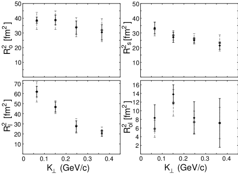
FIG. 1.: The correlation radii in the Cartesian parametrization in the LCMS (see text for details). Black symbols indicate the data points from Table I. Gray dashed symbols represent the values calculated with cross-check relations from the measured YKP parameters given in the Table II.

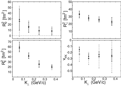
FIG. 2.: The measured YKP parameters, with $v_{{}_{\rm YK}}$ given in the LCMS. Black symbols indicate the data points from Table II. Gray dashed symbols represent the values calculated with cross-check relations from the measured Cartesian parameters given in Table I.

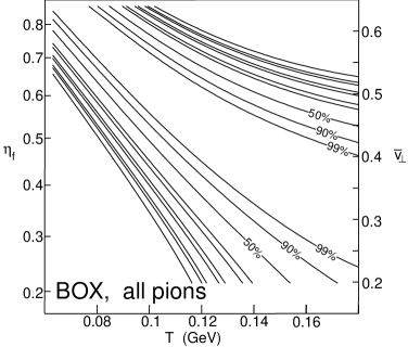
(a)

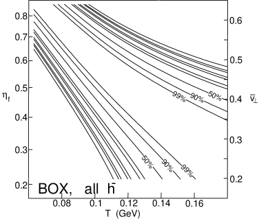
(b)

FIG. 3.: $\chi^{2}$ contour plots for the fit of the single-particle $h^{-}$ spectrum to the model (6) with a box-shaped transverse density profile. The contour lines correspond to the following confidence levels: 99%, 90%, 50%, 10%, 5%, 1%, 0.5%, 0.1%, 0.05%, and 0.01%. Panel (a): fit including all pions. Panel (b): negative hadrons, including also $K^{-}$ and $\bar{p}$ and their resonance decay contributions.

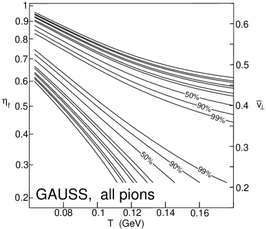
(a)

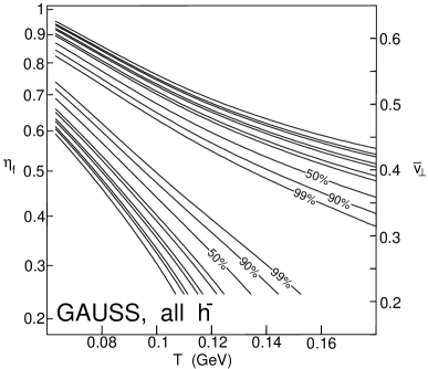
(b)

FIG. 4.: The $\chi^{2}$ contour plots as in Fig. 3 but for the model (6) with Gaussian transverse density profile. The average transverse expansion velocity $\bar{v}_{\perp}$ allows for a direct comparison between the two models. The corresponding values of $\eta_{f}$ are also shown; they differ substantially between the two models.

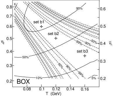
FIG. 5.: $\chi^{2}$ contours for the fit of the Cartesian HBT radii to the model (6) with a box-shaped transverse density profile (solid lines). The numbers give the corresponding confidence levels. The dashed lines show the result of the fit to the single-particle spectrum (Fig. 3b). Crosses denote the positions of the three parameter sets used in further calculations.

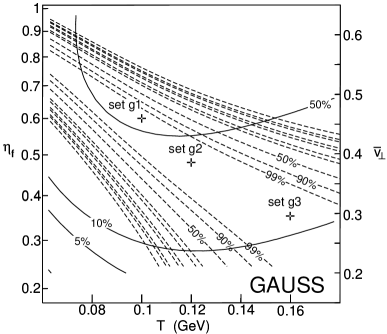
FIG. 6.: Same as Fig. 5 but for the model with a Gaussian transverse density profile.

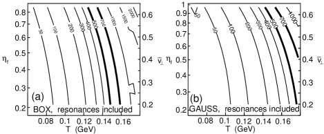
FIG. 7.: Total $\pi^{-}$ multiplicity (resonance decays included) as a function of $T$ and $\bar{v}_{\perp}$, computed from the model with (a) box-shaped, (b) Gaussian transverse density profile. The wiggles in the contours towards the right in panel (a) result from numerical uncertainties in the fitted model parameters. For other details see text.

FIG. 8.: Measured $h^{-}$ spectrum in the rapidity window $4.15{<}y{<}4.65$ [24] compared to the best model fits b1 and g1.

FIG. 9.: Comparison of model predictions from the model with box-shaped transverse geometric profile and inserted parameter sets b1, b2, b3 with the data on Cartesian correlation radii (to which the model was fitted).

FIG. 10.: Same as Fig. 9 but for the Gaussian transverse density profile with parameter sets g1, g2, g3.

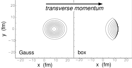
FIG. 11.: Transverse cuts through the effective emission region of particles with $K_{\perp}$=500 MeV/$c$. Left: Gaussian transverse density profile. Right: box-like transverse density profile. In both cases $T$=100 MeV, $\eta_{f}$=0.8.

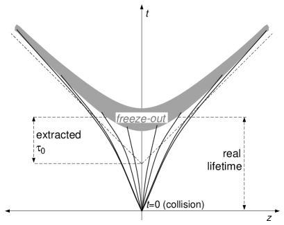
FIG. 12.: Schematic sketch of the interferometric lifetime measurement. The time parameter $\tau_{0}$ is extracted under the assumption that the longitudinal expansion is boost-invariant during the entire dynamical evolution. If the boost-invariant velocity profile develops gradually, the fireball can live longer.

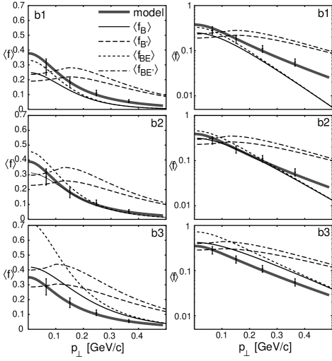
FIG. 13.: Average phase-space density $\langle f\rangle(\leavevmode\text{tensysevensyfivesy\boldmath{$p$}})$ in the rapidity bin $3.9<Y<4.4$ as a function of $p_{\perp}$. The data points are determined from NA49 data (Sec. V B 1). Black lines denote expectations from the statistical treatment in Sec. V B 2: $\langle f_{B}\rangle$ (eq. (48), solid); $\langle f_{B^{\prime}}\rangle$ (eq. (50), long-dashed); $\langle f_{BE}\rangle$ (eq. (49), short-dashed); and $\langle f_{BE^{\prime}}\rangle$ (eq. (51), dash-dotted). Results of our model (see text) are shown by thick solid gray lines. The symbols in the upper right corners indicate the used set of model parameters; the corresponding pionic chemical potentials are listed in Table V. The right column gives a logarithmic representation of the left column.

FIG. 14.: The distribution $\varrho_{2}^{\perp}(K_{\perp})$ of average transverse pair momenta calculated from (A13). The dashed line shows the function $f(K_{\perp})$ from Eq. (A15); the dotted line stands for $g(K_{\perp})$ from (A16). $T_{\rm inv}=185\,\mbox{MeV}$. Longer tics indicate the bin positions for the data in Sec. II.

FIG. 15.: The same as Fig. 14, but all three distributions are divided by $K_{\perp}$ and plotted logarithmically.

FIG. 16.: The chemical potentials $\mu_{B}(T)$ and $\mu_{S}(T)$ in units of $T$ as given by Eqs. (B1) and (B2).

REFERENCES

- [1] Proceedings of the 13th International Conference on Ultra-relativistic Nucleus–Nucleus Collisions: Quark Matter ’97, Tsukuba, Japan, Dec. 1–5, 1997, Nucl. Phys. A638 (1998).
- [2] Proceedings of the 14th International Conference on Ultra-relativistic Nucleus–Nucleus Collisions: Quark Matter ’99, Torino, Italy, May 10–15, 1999, Nucl. Phys. A, in press.
- [3] T. Csörgő and B. Lörstad, Nucl. Phys. A590, 465c (1995).
- [4] T. Csörgő and B. Lörstad, Phys. Rev. C 54, 1390 (1996).
- [5] S. Chapman and J.R. Nix, Phys. Rev. C 56, 866 (1996); J.R. Nix, Phys. Rev. C 58, 2303 (1998).
- [6] U. Heinz, in Hirschegg ’97: QCD Phase Transitions, (H. Feldmeier et al., eds.), GSI report ISSN 0720-9715, 1997, p. 361 (nucl-th/9701054).
- [7] U.A. Wiedemann, B. Tomášik, and U. Heinz, Nucl. Phys. A638, 475c (1998).
- [8] G. Roland et al. (NA49 Coll.), Nucl. Phys. A638, 91c (1998).
- [9] E. Schnedermann, J. Sollfrank, and U. Heinz, Phys. Rev. C 48, 2462 (1993).
- [10] A.N. Makhlin and Yu.M. Sinyukov, Z. Phys. C 39, 69 (1988).
- [11] H. Appelshäuser et al. (NA49 Coll.), Eur. Phys. J. C 2, 643 (1998).
- [12] U.A. Wiedemann and U. Heinz, Phys. Rep., in press (nucl-th/9901094).
- [13] U. Heinz and B.V. Jacak, Ann. Rev. Nucl. Part. Sci. 49 (1999), in press (nucl-th/9902020).
-
[14]
A. Ster, T. Csörgő, and B. Lörstad, in [2]
(hep-ph/9907338). - [15] S. Vörös et al. (WA98 Coll.), in [2].
- [16] I.G. Bearden et al. (NA44 Coll.), Phys. Rev. C 58, 1656 (1998).
- [17] U. Heinz, B. Tomášik, U.A. Wiedemann, and Wu Y.-F., Phys. Lett. B 382, 181 (1996).
- [18] B. Tomášik and U. Heinz, Acta Phys. Slov. 49, 251 (1999).
- [19] B. Tomášik, PhD thesis, Universität Regensburg, 1999.
- [20] R. Ganz et al. (NA49 Coll.), in Proceedings of the 2nd Catania Relativistic Ion Studies (CRIS ’98) (eds. S. Costa et al.), World Scientific, 1999 (nucl-ex/9808006).
- [21] H. Dobler, J. Sollfrank, and U. Heinz, Phys. Lett. B 457, 353 (1999).
- [22] K. Morita, S. Muroya, H. Nakamura, and Ch. Nonaka, nucl-th/9906037.
- [23] G.F. Bertsch, Phys. Rev. Lett. 72, 2349 (1994); 77, 789(E) (1996).
- [24] P.G. Jones et al. (NA49 Coll.), Nucl. Phys. A610, 188c (1996).
- [25] G.D. Lafferty and T.R. Wyatt, Nucl. Instr. and Meth. A 355, 541 (1995).
- [26] H. Appelshäuser et al. (NA49 Coll.), Phys. Rev. Lett. 82, 2471 (1999).
- [27] J. Günther, PhD thesis, Johann Wolfgang Goethe-Universität Frankfurt/Main, 1998 (GSI preprint DISS. 98-14).
-
[28]
S. Schönfelder, PhD thesis, MPI für Physik, München,
1997 (http://na49info.cern.ch/cgi-bin/wwwd-util/
NA49/NOTE?143). - [29] H. Appelshäuser, PhD thesis, Johann Wolfgang Goethe-Universität Frankfurt/Main, 1997 (http://na49info.cern.ch/cgi-bin/wwwd-util/NA49/NOTE?150).
- [30] P. Seyboth, private communication, March 1997.
- [31] Wu Y.-F., U. Heinz, B. Tomášik, and U.A. Wiedemann, Eur. Phys. J. C 1, 599 (1998).
- [32] This is well known to insiders: analogues of Figs. 1 and 2 were shown by K. Kadija (NA49) at the Quark Matter ’96 conference, but unfortunately not included in the proceedings (K. Kadija et al. (NA49), Nucl. Phys. A610, 248c (1996)), nor apparently in any later publications.
- [33] U.A. Wiedemann, P. Scotto, and U. Heinz, Phys. Rev. C 53, 918 (1996).
- [34] B. Tomášik and U. Heinz, Eur. Phys. J. C 4, 327 (1998).
- [35] S. Chapman, P. Scotto, and U. Heinz, Heavy Ion Physics 1, 1 (1995).
- [36] J.D. Bjorken, Phys. Rev. D 27, 140 (1983).
- [37] U.A. Wiedemann and U. Heinz, Phys. Rev. C 56, 3265 (1997).
- [38] T. Csörgő, P. Lévai, and B. Lörstad, Acta Phys. Slov. 46, 585 (1996).
- [39] F. James, MINUIT – Function Minimization and Error Analysis, Reference Manual, CERN, Geneva, 1984; available at http://consult.cern.ch/writeups/minuit/.
- [40] M. Abramowitz and I.A. Stegun, Handbook of Mathematical Functions, Dover Publ., New York, 1965.
- [41] S. Chapman, J.R. Nix, and U. Heinz, Phys. Rev. C 52, 2694 (1995).
- [42] A. Polleri, J.P. Bondorf, and I.N. Mishustin, Phys. Lett. B 419, 19 (1998).
- [43] R. Scheibl and U. Heinz, Phys. Rev. C 59, 1585 (1999).
- [44] H. Heiselberg and A.P. Vischer, Eur. Phys. J. C 1, 593 (1998).
- [45] We gratefully acknowledge a fruitful discussion with H. Sorge on this point.
- [46] S. Pratt, Phys. Lett. B 301, 159 (1993); S. Pratt and V. Zelevinsky, Phys. Rev. Lett. 72, 816 (1994).
- [47] D. Ferenc, U. Heinz, B. Tomášik, U.A. Wiedemann, and J.G. Cramer, Phys. Lett. B 457, 347 (1999).
- [48] F. Cooper and G. Frye, Phys. Rev. D 10, 186 (1974).
- [49] S. Pratt, Phys. Rev. D 33, 72 (1996).
- [50] J. Barrette et al. (E877 Coll.), Phys. Rev. Lett. 78, 2916 (1997).
- [51] C. Slotta, PhD thesis, Universität Regensburg, 1999.
- [52] S. Pratt, in Quark Gluon Plasma 2, (R.C. Hwa, ed.), World Scientific, Singapore, 1995, p. 700.
- [53] H. Bebie, P. Gerber, J.L. Goity, and H. Leutwyler, Nucl. Phys. B378, 95 (1992).
- [54] P. Koch, Phys. Lett. B 288, 187 (1992); Z. Phys. C 57, 283 (1993).
- [55] S. Pratt and K. Haglin, nucl-th/9810051.
- [56] S.E. Vance, T. Csörgő, and D. Kharzeev, Phys. Rev. Lett. 81, 2205 (1998).
- [57] J. Sollfrank, P. Koch, and U. Heinz, Z. Phys. C 52, 593 (1991).
- [58] B. Kämpfer, O.P. Pavlenko, A. Peshier, M. Hentschel, and G. Soff, J. Phys, G 23, 2001 (1997).
- [59] M.M. Aggarwal et al. (WA98 Coll.), nucl-ex/9901009.
- [60] U.A. Wiedemann, in [2] (nucl-th/9907048).
- [61] P. Braun-Munzinger, I. Heppe, and J. Stachel, nucl-th/9903010.
- [62] U.A. Wiedemann, Phys. Rev. C 57, 3324 (1998).
- [63] C.M. Hung and E. Shuryak, Phys. Rev. C 57, 1891 (1998).
- [64] F. Becattini, M. Gaździcki, and J. Sollfrank, Eur. Phys. J. C 5, 143 (1998).
- [65] L. Bravina et al., J. Phys. G 25, 351 (1999).
- [66] J. Bolz et al., Phys. Lett. B 300, 404 (1993); Phys. Rev. D 47, 3860 (1993).
- [67] P. Scotto, PhD thesis, Universität Regensburg, in preparation.