nucl-th/9907077

DOE/ER/40561-33-INT98

NT@UW-99-3

15th July 1999

Quartet $\mathrm{S}$ Wave Neutron Deuteron Scattering in Effective Field Theory

Paulo F. Bedaque${}^{a,\,}$ and Harald W. Grießhammer${}^{b,\,}$

^aInstitute for Nuclear Theory, University of Washington,
Box 351 550, Seattle, WA 98195-1550, USA
^bNuclear Theory Group, Department of Physics, University of Washington,
Box 351 560, Seattle, WA 98195-1560, USA

The real and imaginary part of the quartet $\mathrm{S}$ wave phase shift in $nd$ scattering (${}^{4}\mathrm{S}_{3/2}$) for centre-of-mass momenta of up to $300\;\mathrm{MeV}$ ($E_{\mathrm{cm}}\approx 70\;\mathrm{MeV}$) is presented in effective field theory, using both perturbative pions and a theory in which pions are integrated out. As available, the calculation agrees with both experimental data and potential model calculations, but extends to a higher, so far untested momentum régime above the deuteron breakup point. A Lagrangean more feasible for numerical computations is derived.

Suggested PACS numbers: 11.80.J, 21.30.-x, 21.45.+v, 25.10.+s, 25.40.Dn Suggested Keywords: effective field theory, nucleon-deuteron scattering, three-body systems

1 Introduction

Effective field theory (EFT, for an introduction, see e.g. [1]) methods are largely used in many branches of physics where a separation of scales exists. In low energy nuclear systems, the two well separated scales are, on one side, the low scales of the typical momentum of the process considered and the pion mass, and on the other side the higher scales associated with chiral symmetry and confinement. This separation of scales was explored with great success in the mesonic sector (Chiral Perturbation Theory [2, 3]) and in the one baryon sector (usually by using Heavy Baryon Chiral Perturbation Theory [4, 5]), producing a low energy expansion of a variety of observables. It provided for the first time a systematic, rigorous and model independent (meaning, independent of assumptions about the non-perturbative QCD dynamics) description of strongly interacting particles. A large amount of work was devoted recently to the application of EFT methods to systems containing two nucleons. In the three nucleon sector, some progress was also made in the very low energy range and at low orders where pions do not have to be included explicitly [6, 7]. In this article, we investigate the quartet $\mathrm{S}$ wave of neutron-deuteron scattering using the scheme advanced in [8] in which pions are included perturbatively.

The original suggestion of how to extend EFT methods to systems containing two or more nucleons is due to Weinberg [9] who noticed that below the $\Delta$ production scale, only nucleons and pions need to be retained as the infrared relevant degrees of freedom of low energy QCD. Because at these scales the momenta of the nucleons are small compared to their rest mass, the theory becomes non-relativistic at leading order in the velocity expansion, with relativistic corrections systematically included at higher orders. The most general chirally invariant Lagrangean consists hence of contact interactions between non-relativistic nucleons, and between nucleons and pions. The interactions involving pions are severely restricted by chiral invariance. As such, the theory is an extension to the many nucleon system of Chiral Perturbation Theory and its counterpart in the one nucleon sector, Heavy Baryon Chiral Perturbation Theory. Like in its cousins, all short distance physics – quarks and gluons, resonances like the $\Delta$ or $\sigma$ – is integrated out into the coefficients of the low energy Lagrangean. In principle, these constants could be derived by solving QCD, for example, on the lattice [10]. They can also be determined through models of the short distance physics, like resonance saturation. The most common way to determine those constants, though, is by fitting them to experiment.

Because its Lagrangean consists of infinitely many terms only restricted by symmetry, an effective field theory may at first sight suffer from lack of predictive power. Indeed, as part of its formulation, predictive power is ensured only by establishing a power counting scheme, i.e. a way to determine at which order in a momentum expansion different contributions will appear, and keeping only and all the terms up to a given order. The dimensionless, small parameter on which the expansion is based is the typical momentum $Q$ of the process in units of the scale $\Lambda$ at which the theory is expected to break down, with estimates ranging from $\Lambda\approx 300$ to $800\;\mathrm{MeV}$ [11] in the two body system. Assuming that all contributions are of natural size, i.e. ordered by powers of $Q$, the systematic power counting ensures that the sum of all terms left out when calculating to a certain order in $Q$ is smaller than the last order retained, allowing for an error estimate of the final result.

In systems involving two or more nucleons, establishing such a power counting is complicated by the fact that unnaturally large scales have to be accommodated, so that some coefficients in the Lagrangean may not be of natural size and hence possibly jeopardise power counting: Given that the typical low energy scale in the problem should be the mass of the pion as the lightest particle emerging from QCD, fine tuning seems to be required to produce the large scattering lengths in the ${}^{1}\mathrm{S}_{0}$ and ${}^{3}\mathrm{S}_{1}$ channels ($1/a^{{}^{1}\mathrm{S}_{0}}=-8.3\;\mathrm{MeV},\;1/a^{{}^{3}\mathrm{S}_{1}}=36\;\mathrm{MeV}$). Since there is a bound state in the ${}^{3}\mathrm{S}_{1}$ channel with a binding energy $B=2.225\;\mathrm{MeV}$ and hence a typical binding momentum $\gamma=\sqrt{MB}\simeq 46\mathrm{MeV}$ well below the scale $\Lambda$ at which the theory should break down, it is also clear that at least some processes have to be treated non-perturbatively in order to accommodate the deuteron.

A way to incorporate this fine tuning into the power counting was suggested by Kaplan, Savage and Wise [8]. In it, renormalisation using an unusual subtraction scheme (called Power Divergence Subtraction, PDS) moves a somewhat arbitrary amount of the short distance contributions from loops to counterterms and makes precise cancellations manifest which arise from fine tuning. Power counting then becomes straightforward, but physical observables are of course independent of the renormalisation scale or cut-off chosen. The leading order contribution to nucleons scattering in an $\mathrm{S}$ wave comes from four nucleon contact interactions and is summed geometrically to all orders to produce the shallow real and virtual bound states. Pion interactions and contact operators containing derivatives are suppressed by additional powers of $m_{\pi}$ and $Q$, respectively. In the pion contributions, the exchange of one instantaneous pion is the leading piece, and pion ladders and radiative pions are suppressed further. Dimensional regularisation is chosen to explicitly preserve the systematic power counting as well as all symmetries (esp. chiral invariance) at each order in every step of the calculation. At leading (LO), next-to-leading order (NLO) and often even NNLO in the two nucleon system, this approach also allows in general for simple, closed answers whose analytic structure is readily asserted  [12]. This theory has been put to extensive tests at NLO and NNLO in the two body system, giving for the first time analytic answers to many deuteron properties such as electromagnetic form factors [13], scalar and tensor electromagnetic polarisabilities [14], Compton scattering [15], $np\to d\gamma$ both parity violating [16] and conserving [17], the deuteron anapole moment [18], charge dependence and charge symmetry breaking [19]. The expansion parameter is found to be of the order of $\frac{1}{3}$, so that NLO calculations are accurate to about $10\%$, and NNLO calculations to about $3\%$. In all cases, experimental agreement is within the estimated theoretical uncertainties, and in some cases, previously unknown counterterms could be determined.

Even if calculations of nuclear properties were possible starting from the underlying QCD Lagrangean, effective field theory simplifies the problem considerably by factorising it into a short distance part (subsumed into the coefficient of the Lagrangean) and a long distance part which contains the infrared-relevant physics and is dealt with by effective field theory methods. They provide an answer of finite accuracy because higher order corrections are systematically calculable and suppressed in powers of the expansion parameter $Q$. Hence, the power counting allows for an error estimate of the final result, with the natural size of all neglected terms known to be of higher order. The power of an effective field theory is also that relativistic effects, chiral dynamics and external currents are included systematically, and that extensions to include e.g. parity violating effects are straightforward. Gauged interactions and exchange currents are unambiguous. Results obtained with EFT are easily dissected for the relative importance of the various terms. Because only $S$-matrix elements between on-shell states are observables, ambiguities nesting in “off-shell effects” are absent. On the other hand, because only symmetry considerations enter the construction of the Lagrangean, effective field theories are less restrictive as no assumption about the underlying QCD dynamics is incorporated.

This article presents the first systematic effective field theory calculation of three body properties with pions. For the theory in which pions are integrated out, calculations of three body observables were presented in [7], and $\mathrm{S}$ wave quartet neutron-deuteron scattering was computed up to NNLO below the deuteron breakup threshold. We extend this calculation above threshold and include pions explicitly.

We choose the quartet $\mathrm{S}$ wave channel of $nd$ scattering for this investigation because it provides a laboratory in which many complications of the other channels are not encountered: The absence of Coulomb interactions ensures that only properties of the strong interactions are probed. The Pauli principle forbids three body forces [7] in the first few orders. Because the calculation is parameter-free, it allows one to determine the range of validity of the KSW scheme without a detailed analysis of the fitting procedure. Although the quartet scattering length is large ($1/a^{{}^{4}\mathrm{S}_{\frac{3}{2}}}=31\;\mathrm{MeV}$), no extra fine tuning except the one for the deuteron is required.

The article is organised as follows: After describing the effective theory and its power counting in Sect. 2, we apply it to $nd$ scattering in Sect. 3, followed by a discussion of our results in Sect. 4.

2 The Effective Theory

2.1 Re-formulating the Lagrangean

The first terms in the most general Lagrangean satisfying the QCD symmetries including pions and nucleons are

$$\mathcal{L}_{NN} = N^{\dagger}(\mathrm{i}\partial_{0}+\frac{\vec{\partial}^{2}}{2M})N+\;\frac{f_{\pi}^{2}}{8}\;\mathrm{tr}[(\partial_{\mu}\Sigma^{\dagger})(\partial^{\mu}\Sigma)]+$$

$$+\;\frac{f_{\pi}^{2}}{4}\;\omega\;\mathrm{tr}[\mathcal{M}_{q}(\Sigma^{\dagger}+\Sigma)]+g_{A}N^{\dagger}\vec{A}\cdot\sigma N+$$

$$-\;C_{0}(N^{\mathrm{T}}P^{i}N)^{\dagger}\ (N^{\mathrm{T}}P^{i}N)+\;\frac{C_{2}}{8}\left[(N^{\mathrm{T}}P^{i}N)^{\dagger}(N^{\mathrm{T}}P^{i}(\stackrel{{\scriptstyle\scriptscriptstyle\rightarrow}}{{\partial}}-\stackrel{{\scriptstyle\scriptscriptstyle\leftarrow}}{{\partial}})^{2}N)+\mathrm{h.c.}\right]-$$

$$-\;\omega D_{2}\;\mathrm{tr}[\mathcal{M}_{\mathrm{q}}](N^{\mathrm{T}}P^{i}N)^{\dagger}\ (N^{T}P^{i}N)+\dots\;\;,$$

where $N={p\choose n}$ is the nucleon doublet of two-component spinors and $P^{i}$ is the projector onto the iso-scalar-vector channel,

$$P^{i,\,b\beta}_{a\alpha}=\frac{1}{\sqrt{8}}\;(\sigma_{2}\sigma^{i})_{\alpha}^{\beta}\;(\tau_{2})_{a}^{b}\;\;,$$ (2.2)

$\sigma$ ($\tau$) being the Pauli matrices acting in spin (iso-spin) space. The field $\xi$ describes the pion,

$$\xi(x)=\sqrt{\Sigma}=e^{\mathrm{i}\Pi/f_{\pi}}\;\;,\qquad\Pi=\left(\begin{array}[]{cc}\frac{\pi^{0}}{\sqrt{2}}&\pi^{+}\\ \pi^{-}&-\frac{\pi^{0}}{\sqrt{2}}\end{array}\right)\;\;.$$ (2.3)

$D_{\mu}$ is the chiral covariant derivative $D_{\mu}=\partial_{\mu}+V_{\mu}$, and the vector and axial currents are given by

$$V_{\mu}=\frac{1}{2}(\xi\partial_{\mu}\xi^{\dagger}+\xi^{\dagger}\partial_{\mu}\xi)\;\;,\quad A_{\mu}=\frac{\mathrm{i}}{2}(\xi\partial_{\mu}\xi^{\dagger}-\xi^{\dagger}\partial_{\mu}\xi)\;\;.$$ (2.4)

The pion decay constant is normalised to be $f_{\pi}=130\;\mathrm{MeV}$, $\mathcal{M}_{\mathrm{q}}=\mathrm{diag}(m_{\mathrm{u}},m_{\mathrm{d}})$ is the quark mass matrix, and the constant $\omega$ is chosen such that $m_{\pi}^{2}=\omega(m_{\mathrm{u}}+m_{\mathrm{d}})$. From now on, we split the coefficient of the leading four point interaction, $C_{0}$, into a leading ($C_{0}^{(-1)}$) and a sub-leading piece ($C_{0}^{(0)}$) and absorb $D_{2}$ into $C_{0}^{(0)}$ since these two terms can be distinguished only in processes involving two or more pions sensitive to explicit chiral symmetry breaking by the finite quark masses that will not appear here.

The Lagrangean has all the symmetries of QCD, including $SU(2)_{\mathrm{L}}\times SU(2)_{\mathrm{R}}$ chiral invariance under which the pion and nucleon fields transform as

$$\xi\rightarrow L\xi U^{\dagger}=U\xi R^{\dagger}\;\;,\qquad\Sigma\rightarrow L\Sigma R^{\dagger}\;\;,\qquad N\rightarrow UN\;\;,$$ (2.5)

where $L$ and $R$ are constant $SU(2)$ matrices and $U$ is a complicated, $SU(2)$ matrix-valued function of $L,\;R$ and the pion fields. The chiral Lagrangean differs from the one used in Heavy Baryon Chiral Perturbation Theory by the inclusion of four and other multi-nucleon contact forces, the latter of which are not explicitly shown here.

We now recapitulate the scaling properties of the operators in the Lagrangean (2.1) necessary to establish the power counting in the next section as suggested by Kaplan, Savage and Wise [8]. Because momenta scale like $Q$ and energies like $Q^{2}/M$ in the non-relativistic régime, naïve dimensional arguments suggest that the two-nucleon force term with $n$ derivatives should scale as

$$C_{n}\sim\frac{1}{M\Lambda^{n+1}}\;\;.$$ (2.6)

However, the existence of unnaturally shallow bound states and large scattering lengths indicates the presence of fine tuning. The inverse deuteron size is $\gamma=46\;\mathrm{MeV}$ and the scattering length in the nucleon-nucleon singlet channel is $\sim 24$ fm, both of which are certainly not typical QCD scales. Most likely, these small scales do not arise from the fact that the real world is close to the chiral limit: In the singlet channel, for instance, the one pion exchange potential vanishes in the chiral limit and thus cannot be the cause of the fine tuning. The fine tuning then must be a result of short distance physics. This, in turn, implies that a naïve estimate of sizes of graphs and counterterms using (2.6) may be misleading due to precise cancellations and/or enhancements. The exact nature of these cancellations and/or enhancements depends on the particular way the short distance physics contribution is split between loops and counterterms and, consequently, acquires different forms in different regularisation and subtraction schemes. Using a cut-off scheme, for example, the sizes of the coefficients $C_{n}$ satisfy (2.6) with $\Lambda$ the cut-off scale, but they are fine tuned in such a way that sums of diagrams are parametrically larger/smaller than each diagram individually, complicating the power counting. It is also hard to keep chiral and gauge invariance with those regulators. One convenient way of keeping track of the new scale generated by the fine tuning was suggested by Kaplan, Savage and Wise [8]. It consists in the use of dimensional regularisation and of a subtraction scheme called Power Divergence Subtraction (PDS), in which not only the pole present in $4$ dimensions is subtracted (as in the minimal subtraction scheme), but also poles present in $3$ dimensions (finite pieces in $4$ dimensions) are removed. This unusual subtraction scheme re-shuffles a finite piece of the short distance contributions from loops to counterterms and changes the scaling of the short distance constants from (2.6) to

$$C_{0}^{(-1)} \sim \frac{1}{MQ}\;\;,$$

$$C_{0}^{(0)} \sim \frac{1}{M\Lambda}\;\;,$$ (2.7)

$$C_{2} \sim \frac{1}{M\Lambda Q^{2}}\;\;.$$

Here, $Q$ stands for a low energy scale like the external momenta, the inverse scattering length or the pion mass. Other, equivalent ways of accomplishing the same result by performing a subtraction at finite off-shell momenta were suggested, too [20, 21]. One surprising result arises from this analysis because chiral symmetry implies a derivative coupling of the pion to the nucleon at leading order. The contribution from one pion exchange includes a factor of $Q^{-2}$ from the pion propagator and a factor of $Q^{2}$ coming from the pion-nucleon vertices, so that for momenta of the order of the pion mass, the one pion exchange scales as $Q^{0}$ and is smaller than the contact piece $C_{0}^{(-1)}$ which according to (2.1) scales as $Q^{-1}$. Iterated pion exchanges are suppressed even further. On the other hand, repeated iterations of the $C_{0}^{(-1)}$ term are not suppressed, and the two-nucleon system is described at leading order by an infinite number of iterations of the leading contact interaction, as will be demonstrated below. Pion exchange and higher derivative contact terms appear hence only as perturbations at higher orders. In this scheme, the only non-perturbative physics responsible for nuclear binding is extremely simple, and the more complicated pion contributions are at each order given by a finite number of diagrams. In the two body sector, this simplification allows for the derivation of simple analytic expressions of deuteron observables. In the three body sector discussed in this paper, even the leading order calculation will turn out to be too complex for a fully analytical solution. Still, the equations that need to be solved are computationally trivial and can furthermore be improved systematically by higher order corrections that involve only (partly analytical, partly numerical) integrations, as opposed to many-dimensional integral equations arising in other approaches.

The estimate of the three-nucleon force terms is also influenced by the fine tuning in the two-nucleon sector. In the quartet channel though, where the spin of the three participating nucleons are aligned, the Pauli principle forbids a contribution from the contact three body force without derivatives. The remaining ones are suppressed and do not contribute to the order we are working here.

For our purposes, it is convenient to use a Lagrangean equivalent to (2.1) containing an additional field $d^{i}$ carrying the quantum numbers of the deuteron, such that the four nucleon contact interactions are removed:

$$\mathcal{L}_{Nd} = N^{\dagger}(\mathrm{i}\partial_{0}+\frac{\vec{\partial}^{2}}{4M})N+d^{i\dagger}\left[w(\mathrm{i}\partial_{0}+\frac{\nabla^{2}}{4M})-\Delta^{(-1)}-\Delta^{(0)}\right]d^{i}+$$ (2.8)

$$+\;y\left[d^{i\dagger}(N^{\mathrm{T}}P^{i}N)+\mathrm{h.c.}\right]+\dots\;\;,$$

where

$$w = -1\;\;,$$

$$y^{2} = \frac{(C_{0}^{(-1)})^{2}}{MC_{2}}\;\;,$$

$$\Delta^{(-1)} = -\frac{C_{0}^{(-1)}}{MC_{2}}\;\;,$$ (2.9)

$$\Delta^{(0)} = \frac{C_{0}^{(0)}}{MC_{2}}\;\;,$$

and the pion nucleon interactions are still given by the terms of (2.1). Analogously to $C_{0}$, we split $\Delta$ into a leading ($\Delta^{(-1)}$) and a sub-leading piece ($\Delta^{(0)}$). The “wrong” sign in the kinetic term for $w=-1$ does not spoil unitarity as can be seen from the equivalence of (2.1) and (2.8) proven below. Using (2.1) and the scaling of the constants $C_{0}^{(-1)},\;C_{0}^{(0)}$ and $C_{2}$ in the KSW scheme, we find

$$\Delta^{(-1)} \sim \frac{Q\Lambda}{M}\;\;,$$

$$\Delta^{(0)} \sim \frac{Q^{2}}{M}\;\;,$$ (2.10)

$$y^{2} \sim \frac{\Lambda}{M^{2}}\;\;.$$

The Lagrangean in (2.8) is not the most general one involving nucleons, pions and “deuteron” fields. Since this Lagrangean contains more fields than the minimum number necessary, there is a large reparametrisation invariance that can be used to choose the coefficients of some terms to vanish. This freedom in rewriting equivalent Lagrangeans will be used later to accomplish non-trivial rearrangements of diagrams in order to simplify computations. To see the equivalence of (2.8) and (2.1), we simply perform the Gaußian integration over the field $d^{i}$ in the path integral. After eliminating the terms containing time derivatives by a field re-definition

$$N \rightarrow N+\frac{y^{2}}{8\ (\Delta^{(-1)})^{2}}\;P^{i\dagger}N^{\dagger}(N^{\mathrm{T}}P^{i}N)\;\;,$$

$$N^{\dagger} \rightarrow N^{\dagger}+\frac{y^{2}}{8\ (\Delta^{(-1)})^{2}}\;(N^{\mathrm{T}}P^{i}N)^{\dagger}P^{i}N\;\;,$$ (2.11)

and using (2.1) we are left with (2.1) plus i) terms of higher order, ii) a three-nucleon force term with no derivatives that does not contribute to the quartet scattering, and iii) multi-nucleon forces not relevant to the three-nucleon system. Because all those contributions can be absorbed into terms present already in (2.1) the two formulations of the theory are therefore indeed equivalent. The choice of (2.8) itself is of course not unique. For example, the kinetic term of the deuteron field could have been dropped in favour of keeping the $C_{2}$ term of the nuclear four point interaction. We choose this form for practical reasons related to the numerical integration, as will become apparent later.

2.2 Power Counting and Parameter Determination

We will briefly state the power counting used here and discuss a couple of examples that will be relevant later. More details can be found in [8]. We need to determine the scaling of different contributions as the external momenta $p$, the inverse scattering length $a^{{}^{3}S_{1}}$ and the pion mass go to zero in order to estimate their relative importance. We will take $p\sim 1/a^{{}^{3}S_{1}}\sim m_{\pi}$ and denote this scale by $Q$. Our expansion will be in powers of $Q/\Lambda\sim p/\Lambda\sim 1/(a^{{}^{3}S_{1}}\Lambda)\sim m_{\pi}/\Lambda$, but powers of $p\,a^{{}^{3}S_{1}}\sim m_{\pi}a^{{}^{3}S_{1}}\sim 1$ will be kept to all orders.

It is straightforward to estimate the loop contributions: Because the theory is non-relativistic, the typical energies of on-shell nucleons are of the order $Q^{2}/M$. Thus, the leading contribution of a diagram can be found by scaling all momenta by a factor of $Q$ and all energies by a factor of $Q^{2}/M$. The remaining integral includes no dimensions and is taken to be of the order $Q^{0}$ and of natural size. This scaling implies the rule that nucleon propagators contribute one power of $M/Q^{2}$ and each loop a power of $Q^{5}/M$. Other régimes, in which loop four momenta scale as $Q\sim m_{\pi}$ (on-shell propagation of pions in loops) or as $\sqrt{Mm_{\pi}}$ (pion exchanges with momenta close to the pion production threshold), can be shown not to contribute to the order considered here [22, 23]. The vertices provide powers of $Q$ according to (2.1), implying that the deuteron kinetic energy is sub-leading compared to the $\Delta^{(-1)}$ term. Thus, the bare deuteron propagator is just the constant $-\mathrm{i}/\Delta^{(-1)}$. Using these rules, we find the diagrams contributing at leading order to the deuteron propagator to be an infinite number as shown in Fig. 1, each one of the order $1/(MQ)$.

(40,40) i o double,width=thini,o   $=$   (40,40) i o vanilla,width=1.5*thicki,o   $+$   (40,40) i o vanilla,width=1.5*thick,tension=5i,v1 vanilla,width=1.5*thick,tension=5o,v2 vanilla,width=thin,left=0.65v1,v2 vanilla,width=thin,left=0.65v2,v1   $+$   (70,40) i o vanilla,width=1.5*thick,tension=5i,v1 vanilla,width=1.5*thick,tension=5v2,v3 vanilla,width=1.5*thick,tension=5v4,o vanilla,width=thin,left=0.65v1,v2 vanilla,width=thin,left=0.65v2,v1 vanilla,width=thin,left=0.65v3,v4 vanilla,width=thin,left=0.65v4,v3   $+$   (100,40) i o vanilla,width=1.5*thick,tension=5i,v1 vanilla,width=1.5*thick,tension=5v2,v3 vanilla,width=1.5*thick,tension=5v4,v5 vanilla,width=1.5*thick,tension=5v6,o vanilla,width=thin,left=0.65v1,v2 vanilla,width=thin,left=0.65v2,v1 vanilla,width=thin,left=0.65v3,v4 vanilla,width=thin,left=0.65v4,v3 vanilla,width=thin,left=0.65v5,v6 vanilla,width=thin,left=0.65v6,v5   $+\;\dots$

Figure 1: The deuteron propagator at leading order from the Lagrangean (2.8). The thick solid line denotes the bare propagator $\frac{-\mathrm{i}}{\Delta^{(-1)}}$, the double line its dressed counterpart.

The linear divergence in each of the bubble diagrams shown in Fig. 1 does not show in dimensional regularisation as a pole in $4$ dimensions, but it does appear as a pole in $3$ dimensions which we subtract following the PDS scheme discussed above. In other regularisation or subtraction schemes, each term in the series depicted in Fig. 1 would contribute with a different power of $Q$, starting with the first, tree level diagram that would be of the order $1/(M\Lambda)$. Their sum, however, will still scale as $1/(MQ)$, exemplifying the precise cancellation discussed above, see e.g. [24].

The full leading order propagator $\mathrm{i}\triangle^{ij}(p)$ of the deuteron field consists hence of the geometric series shown in Fig. 1,

$$\mathrm{i}\triangle^{ij}(p)=-\;\frac{4\pi\mathrm{i}}{My^{2}}\;\frac{\delta^{ij}}{\frac{4\pi\Delta^{(-1)}}{My^{2}}-\mu+\sqrt{\frac{\vec{\,\!p}\!\>{}^{2}}{4}-Mp_{0}-\mathrm{i}\varepsilon}}\;\;.$$ (2.12)

At leading order, all physical quantities will therefore depend on the parameters $y$ and $\Delta^{(-1)}$ only through the combination $C_{0}^{(-1)}=-y^{2}/\Delta^{(-1)}$, so that there is only one free parameter in the effective theory. Either $y$ or $\Delta^{(-1)}$ can hence be chosen at will. This is clear since the same results could have been obtained directly from (2.1) where only $C_{0}^{(-1)}$ appears. We determine this parameter from the binding energy of the deuteron, i.e. from the position of the pole of $\mathrm{i}\triangle(p)$:

$$C_{0}^{(-1)}=-\frac{y^{2}}{\Delta^{(-1)}}=\frac{4\pi}{M}\;\frac{1}{\gamma-\mu}$$ (2.13)

Eq. (2.12) confirms the necessity to re-sum the “bubble chain” with $C_{0}^{(-1)}$ interactions to all orders when considering momenta $p\sim\gamma$ and the scaling of $C_{0}^{(-1)}$ with $Q^{-1}$ when choosing as subtraction point $\mu=m_{\pi}\sim Q$, in agreement with the claim made previously. We will keep $\mu=m_{\pi}$ throughout this article. By attaching nucleon external lines to $\mathrm{i}\triangle(p)$, we obtain the nucleon-nucleon scattering amplitude which, at this leading order, is simply the effective range expansion truncated at the first term,

$$\mathcal{A}^{(-1)}=-\;\frac{4\pi}{M}\;\frac{1}{\gamma+ip}\;\;.$$ (2.14)

Looking at (2.12), we derive the final rule for the power counting: Each deuteron propagator is accompanied by a power of $1/(My^{2}Q)=M/(\Lambda Q)$.

At NLO, there are four free parameters in the Lagrangean (2.8), $\Delta^{(-1)},\;\Delta^{(0)},\;y$ and $w$, but only three in the equivalent Lagrangean (2.1). Therefore, one of the parameters is again arbitrary. We choose to fix the only dimensionless one, $w=-1$, giving the deuteron a kinetic energy term with a supposedly wrong sign. Still, because the two Lagrangeans are equivalent, unitarity and causality are not violated. The splitting of $\Delta=\Delta^{(-1)}+\Delta^{(0)}$ between $\Delta^{(-1)}$ and $\Delta^{(0)}$ is also arbitrary. We choose to keep $\Delta^{(-1)}$ the same as at leading order, so that (2.13) is still valid at NLO and higher order calculations will not necessitate a re-fitting of lower order coefficients [25]. The remaining piece, $\Delta^{(0)}$, is then parametrically smaller (as indicated by (2.1)) and is included perturbatively. In a NNLO calculation, $C_{2}$ would be split in a likewise fashion, with $C_{2}^{(0)}$ still given by the expression below, $C_{2}^{(1)}$ to be determined anew, and so on.

The two extra conditions we use to determine the constants $\Delta^{(0)}$ and $y$ are that the position of the deuteron pole $\gamma$, which is already reproduced at LO by $\Delta^{(-1)}$, is unchanged, and that the nucleon-nucleon scattering length in the triplet channel, $a^{{}^{3}\mathrm{S}_{1}}$, is reproduced.

The condition for the pole position (Fig. 2) implies with $w=-1$ and $\mu=m_{\pi}$ (See the later, full calculation of the deuteron corrections at NLO in Sect. 3.)

$$\Delta^{(0)}=\frac{\gamma^{2}}{M}-\frac{y^{2}g_{A}^{2}m_{\pi}^{2}}{32\pi^{2}f_{\pi}^{2}}\left[(\gamma-m_{\pi})^{2}+m_{\pi}^{2}\left(\ln(1+\frac{2\gamma}{m_{\pi}})-1\right)\right]\;\;.$$ (2.15)

The first term in brackets comes from the $\delta$ function part of the pion exchange, the second one from the Yukawa part.

$\left[\mbox{\parbox{40.0pt}{ \fmfgraph*(40,20) \fmfleft{i} \fmfright{o} \fmf{double,width=thin}{i,v1,o} \fmfblob{8*thick}{v1} }}\right]^{-1}\bigg{|}_{p_{0}=-\frac{\gamma^{2}}{M},\,\vec{\,\!p}\!\>{}=0}\stackrel{{\scriptstyle!}}{{=}}0$   :

$\left[\mbox{\parbox{40.0pt}{ \fmfgraph*(40,20) \fmfleft{i} \fmfright{o} \fmf{double,width=thin}{i,o} }}\right]^{-1}\bigg{|}_{p_{0}=-\frac{\gamma^{2}}{M},\atop\,\vec{\,\!p}\!\>{}=0}\stackrel{{\scriptstyle!}}{{=}}0$     ,    $\left[\hskip 5.0pt\mbox{\parbox{40.0pt}{ \fmfgraph*(40,40) \fmfleft{i} \fmfright{o} \fmf{double,width=thin}{i,v1,o} \fmfv{decoration.shape=cross,decor.size=6*thick, label=$\scriptstyle\mathrm{i}w(p_{0}-\frac{\vec{\,\!p}\!\>{}^{2}}{4M})$,label.angle=90}{v1} }}\hskip 5.0pt+\hskip 5.0pt\mbox{\parbox{40.0pt}{ \fmfgraph*(40,40) \fmfleft{i} \fmfright{o} \fmf{double,width=thin}{i,v1,o} \fmfv{decoration.shape=circle,decor.filled=empty, decor.size=3*thick, label=$\scriptstyle-\mathrm{i}\Delta^{(0)}$,label.angle=90}{v1} }}\hskip 5.0pt+\hskip 5.0pt\mbox{\parbox{60.0pt}{ \fmfgraph*(60,40) \fmfleft{i} \fmfright{o} \fmf{double,width=thin,tension=8}{i,v1} \fmf{double,width=thin,tension=8}{v2,o} \fmf{vanilla,width=thin,left=0.65}{v1,v2} \fmf{vanilla,width=thin,left=0.65}{v2,v1} \fmffreeze\fmffreeze\fmfipath{pa} \fmfiset{pa}{vpath(__v1,__v2)} \fmfipath{pb} \fmfiset{pb}{vpath(__v2,__v1)} \fmfi{dashes,foreground=red}{point 1/2 length(pa) of pa -- point 1/2 length(pb) of pb} }}\hskip 5.0pt\right]_{p_{0}=-\frac{\gamma^{2}}{M},\atop\,\vec{\,\!p}\!\>{}=0}\stackrel{{\scriptstyle!}}{{=}}0$

Figure 2: The first condition on the coefficients $\Delta^{(-1)},\,\Delta^{(0)}$ and $y$, (2.13/2.15). The dressed deuteron propagator has its pole at the physical binding energy at LO, and higher order corrections do not change its position. The cross denotes an energy insertion proportional to $w$, the dot an insertion of $\Delta^{(0)}$.

Imposing the experimental value of the triplet nucleon-nucleon scattering length gives a second condition (Fig. 3):

$$\frac{4\pi}{M}a^{{}^{3}\mathrm{S}_{1}}=\frac{4\pi}{M}\left[\frac{1}{\gamma}+\frac{4\pi}{M}\frac{\Delta^{(0)}}{y^{2}\gamma^{2}}\right]$$ (2.16)

Pion contributions do not appear in (2.16) because they vanish at zero momentum in the subtraction scheme used here, the Yukawa piece cancelling against the “$\delta$ function at the origin” part.

(60,30) i1,i2 o1,o2 vanilla,width=thini1,v1 vanilla,width=thini2,v1 vanilla,width=thino1,v2 vanilla,width=thino2,v2 double,width=thin,tension=0.5v1,v2 $+$ (60,30) i1,i2 o1,o2 vanilla,width=thini1,v1 vanilla,width=thini2,v1 vanilla,width=thino1,v2 vanilla,width=thino2,v2 double,width=thinv1,v3,v2 decoration.shape=cross,decor.size=6*thickv3 $+$ (60,30) i1,i2 o1,o2 vanilla,width=thini1,v1 vanilla,width=thini2,v1 vanilla,width=thino1,v2 vanilla,width=thino2,v2 double,width=thinv1,v3,v2 decoration.shape=circle,decor.filled=empty, decor.size=3*thickv3 $+$

$+$ (60,30) i1,i2 o1,o2 vanilla,width=thini1,v1,o1 vanilla,width=thini2,v2,o2 dashes,width=thin,foreground=redv1,v2 $+\;2$ (60,30) i1,i2 o1,o2 vanilla,width=thini1,v1 vanilla,width=thini2,v1 vanilla,width=thin,tension=3o1,v3 vanilla,width=thinv3,v2 vanilla,width=thin,tension=3o2,v4 vanilla,width=thinv4,v2 double,width=thinv1,v2 dashes,width=thin,foreground=redv3,v4 $+$ (80,30) i1,i2 o1,o2 vanilla,width=thini1,i0,i2 vanilla,width=thino1,o0,o2 double,width=thin,tension=2i0,v1 double,width=thin,tension=2v2,o0 vanilla,width=thin,left=0.65,tension=0.3v1,v2 vanilla,width=thin,left=0.65,tension=0.3v2,v1 pa pavpath(__v1,__v2) pb pbvpath(__v2,__v1) dashes,foreground=redpoint 1/2 length(pa) of pa – point 1/2 length(pb) of pb

Figure 3: $NN$ scattering at NLO gives the second condition on the coefficients $\Delta^{(0)}$ and $y$, (2.16): The scattering length has the experimental value. Notation as in Fig. 2.

Solving (2.15) and (2.16) together with (2.13) leads to

$$y^{2} = \frac{4\pi}{M^{2}}\;\frac{\gamma}{G}\;\;,$$

$$\Delta^{(-1)} = \frac{(m_{\pi}-\gamma)\gamma}{M}\;\frac{1}{G}\;\;,$$ (2.17)

$$\Delta^{(0)} = \frac{\gamma^{2}}{M}\;\frac{\gamma a^{{}^{3}\mathrm{S}_{1}}-1}{G}\;\;,$$

with

$$G=\gamma a^{{}^{3}\mathrm{S}_{1}}-1+\frac{g_{A}^{2}M}{8\pi f_{\pi}^{2}\gamma}\left[(\gamma-m_{\pi})^{2}+m_{\pi}^{2}\left(\ln[1+\frac{2\gamma}{m_{\pi}}]-1\right)\right]\;\;.$$ (2.18)

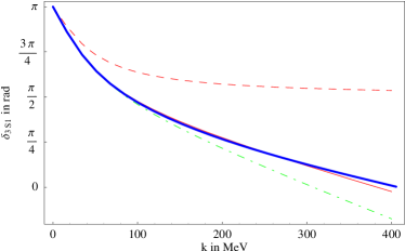
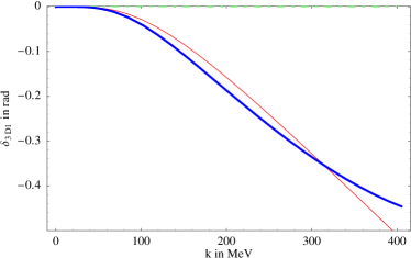
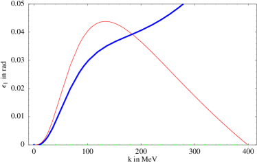
Figure 4: The ${}^{3}S_{1}$ and ${}^{3}D_{1}$ phase shifts in the $NN$ system and the mixing angle $\epsilon_{1}$ obtained with the parameters determined as described in the text. The dashed line is the LO result, the thin solid (dot-dashed) line the NLO result with perturbative pions (pions integrated out), and the thick solid line the Nijmegen phase shift analysis [26].

Figure 4 shows that the resulting phase shifts for $NN$ scattering in the ${}^{3}\mathrm{S}_{1}-{}^{3}\mathrm{D}_{1}$ system and its mixing parameter is in good agreement with the Nijmegen partial wave analysis [26]. When pions are integrated out, the phase shift of the ${}^{3}D_{1}$ channel and the ${}^{3}S_{1}-{}^{3}D_{1}$ mixing angle are identical to zero at NLO. At LO, both quantities vanish, too.

3 Three Body Scattering at NLO

Let us now look at the diagrams contributing to neutron-deuteron scattering in the quartet channel. One might guess from the two-nucleon scattering experience that all the graphs involving only $y$ and $\Delta^{(-1)}$ (e.g.  the ones in the first line in Fig. 5) contribute at leading order, and the deuteron kinetic energy, pion exchanges and the $\Delta^{(0)}$ term appear at NLO. Indeed, following the rules discussed above, we can verify that the tree level diagram is proportional to $y^{2}M/Q^{2}\sim\Lambda/(MQ^{2})$. The $n$-loop diagram with a bare deuteron propagator is proportional to $y^{2+2n}(1/\Delta^{(-1)})^{n}(M/Q^{2})^{1+2n}(Q^{5}/M)^{n}\sim\Lambda/(MQ^{2})$ and hence contributes at the same order. Dressing the deuteron propagator as in Fig. 1 does not change the order of the diagram since it only changes the bare propagator $-\mathrm{i}/\Delta^{(-1)}\sim M/(Q\Lambda)$ by the dressed propagator $\mathrm{i}\triangle(p)\sim 1/(My^{2}Q)\sim M/(Q\Lambda)$. The infinite number of graphs shown in Fig. 5 contributing at leading order forms therefore a double infinite series.

(50,50) i2,i1 o2,o1 vanilla,width=1.5*thick,tension=6i1,v1,v2 vanilla,width=thinv2,o1 vanilla,width=1.5*thick,tension=6v3,v4,o2 vanilla,width=thini2,v3 vanilla,width=thinv2,v3 $+$ (90,50) i2,i1 o2,o1 vanilla,width=1.5*thick,tension=4i1,v1 vanilla,width=thinv1,v2 vanilla,width=1.5*thick,tension=4o1,v2 vanilla,width=1.5*thick,tension=4v3,v4 vanilla,width=thini2,v3 vanilla,width=thinv4,o2 vanilla,width=thinv2,v4 vanilla,width=thinv3,v1 $+$ (130,50) i2,i1 o2,o1 vanilla,width=1.5*thick,tension=8i1,v1 vanilla,width=thinv1,v2 vanilla,width=1.5*thick,tension=8o1,v2 vanilla,width=1.5*thick,tension=4v3,v3a vanilla,width=1.5*thick,tension=4v4,v4a phantomv3a,v4a vanilla,width=thini2,v3 vanilla,width=thinv4,o2 vanilla,width=thinv2,v4 vanilla,width=thinv3,v1 vanilla,width=thin,left=0.65v3a,v4a vanilla,width=thin,left=0.65v4a,v3a $+$ (130,50) i2,i1 o2,o1 vanilla,width=1.5*thick,tension=8i1,v1 vanilla,width=thinv1,v4 vanilla,width=1.5*thick,tension=8v4,v5 vanilla,width=thin,tension=1.666v5,o1 vanilla,width=1.5*thick,tension=8o2,v6 vanilla,width=thinv6,v3 vanilla,width=1.5*thick,tension=8v3,v2 vanilla,width=thin,tension=1.666v2,i2 vanilla,width=thinv1,v2 vanilla,width=thinv3,v4 vanilla,width=thinv5,v6 $+\;\dots$

(104,64) i2,i1 o2,o1 label=$\scriptstyle(\frac{3\vec{k}^{2}}{4M}-\frac{\gamma^{2}}{M},,\vec{k})$, label.angle=90i1 label=$\scriptstyle(\frac{3\vec{k}^{2}}{4M}-\frac{\gamma^{2}}{M}+\epsilon,,\vec{\,\!p}\!\>{})$,label.angle=90o1 label=$\scriptstyle(\frac{\vec{k}^{2}}{2M},,-\vec{k})$,label.angle=-90i2 label=$\scriptstyle(\frac{\vec{k}^{2}}{2M}-\epsilon,,-\vec{\,\!p}\!\>{})$, label.angle=-90o2 double,width=thin,tension=3i1,v1 double,width=thin,tension=1.5v1,v3,v2 double,width=thin,tension=3v2,o1 vanilla,width=thini2,v4,o2 ellipse,foreground=red,rubout=1v3,v4   $=$   (104,64) i2,i1 o2,o1 double,width=thin,tension=4i1,v1,v2 vanilla,width=thinv2,o1 double,width=thin,tension=4v3,v4,o2 vanilla,width=thini2,v3 vanilla,width=thinv2,v3   $+$   (192,64) i2,i1 o2,o1 double,width=thin,tension=3i1,v1 double,width=thin,tension=1.5v1,v6,v5 double,width=thin,tension=3v5,v2 vanilla,width=thinv2,o1 vanilla,width=thini2,v7 vanilla,width=thin,tension=0.666v7,v4 double,width=thin,tension=4v4,v3,o2 vanilla,width=thinv4,v2 ellipse,foreground=red,rubout=1v6,v7

Figure 5: The double infinite series of LO “pinball” diagrams, some of which are shown in the first line, is equivalent to the solution of the Faddeev equation (3) shown in the second line. Notation as in Fig. 2.

First, all “bubble chain” graphs are re-summed into the leading order deuteron propagator $\mathrm{i}\triangle(p)$. Then, the kernel made of $\mathrm{i}\triangle(p)$ and the propagator of the nucleon exchanged is iterated an arbitrary number of times. We are hence left with the task of summing all the diagrams depicted in the first line of Fig. 5. In contradistinction to the two-nucleon case, they do not form a geometric series and cannot be summed analytically. However, one can obtain the solution numerically from the integral equation pictorially shown in the lower line of Fig 5. To derive this equation for the half off-shell amplitude at LO, let us choose the kinematics as in Fig. 5 in such a way that the incoming (outgoing) deuteron line carries momentum $\vec{k}$ ($\vec{\,\!p}\!\>{}$), energy $3\vec{k}^{2}/(4M)-\gamma^{2}/M$ ($3\vec{k}^{2}/(4M)-\gamma^{2}/M+\epsilon$) and vector index $i$ ($j$). The incoming (outgoing) nucleon line carries momentum $-\vec{k}$ ($-\vec{\,\!p}\!\>{}$), energy $\vec{k}^{2}/(2M)$ ($\vec{k}^{2}/(2M)-\epsilon$) and spinor and iso-spinor indices $\alpha$ and $a$ ($\beta$ and $b$). Hence, the incoming deuteron and nucleon are on shell, and $\epsilon$ denotes how far the outgoing particles are off shell. We denote by $\mathrm{i}t_{\alpha a}^{ij\ \beta b}(\vec{k},\vec{\,\!p}\!\>{},\epsilon)$ the sum of those diagrams with the kinematics above and read off from the lower line of Fig. 5 the integral equation for the half off-shell amplitude:

$$\mathrm{i}t_{\alpha a}^{ij\ \beta b}(\vec{k},\vec{\,\!p}\!\>{},\epsilon) = \frac{y^{2}}{2}\;(\sigma^{j}\sigma^{i})_{\alpha}^{\beta}\;\delta_{a}^{b}\;\frac{\mathrm{i}}{-\frac{\vec{k}^{2}}{4}-\frac{\gamma^{2}}{M}+\epsilon-\frac{(\vec{k}+\vec{\,\!p}\!\>{})^{2}}{M}+\mathrm{i}\varepsilon}+$$

$$+\;\frac{y^{2}}{2}\;(\sigma^{j}\sigma^{k})_{\gamma}^{\beta}\;\delta_{c}^{b}\;\int\frac{d^{4}q}{(2\pi)^{4}}\ \mathrm{i}t_{\alpha a}^{ik\ \gamma c}(\vec{k},\vec{\,\!q}\!\>{},\epsilon+q_{0})\ \mathrm{i}\triangle(\frac{\vec{k}^{2}}{4}-\frac{\gamma^{2}}{M}+\epsilon+q_{0},\vec{\,\!q}\!\>{})\;\times$$

$$\phantom{4y^{2}(\sigma^{j}\sigma^{k})_{\gamma}^{\beta}}\times\;\frac{\mathrm{i}}{\frac{\vec{k}^{2}}{2M}-\epsilon-q_{0}-\frac{\vec{\,\!q}\!\>{}^{2}}{2M}+\mathrm{i}\varepsilon}\ \frac{\mathrm{i}}{-\frac{\vec{k}^{2}}{4M}-\frac{\gamma^{2}}{M}+2\epsilon+q_{0}-\frac{(\vec{\,\!q}\!\>{}+\vec{\,\!p}\!\>{})^{2}}{2M}}\;\;.$$

The integration over $q_{0}$ picks the pole at $q_{0}=(\vec{k}^{2}-\vec{\,\!q}\!\>{}^{2})/(2M)-\epsilon+\mathrm{i}\varepsilon$. After that, we set $\epsilon=(\vec{k}^{2}-\vec{\,\!p}\!\>{}^{2})/(2M)$, integrate over the angle between $\vec{k}$ and $\vec{\,\!p}\!\>{}$ to project onto the $\mathrm{S}$ wave, and set $i=(1+\mathrm{i}2)/\sqrt{2},\;j=(1-\mathrm{i}2)/\sqrt{2},\;\alpha=\beta=1,\;a=b=1$, to pick up the spin quartet part. Denoting this projected amplitude by $\mathrm{i}t_{0}(k,p)$, we find

$$t_{0}(k,p) = -\;\frac{y^{2}M}{2pk}\ln\left[\frac{p^{2}+pk+k^{2}-ME-\mathrm{i}\varepsilon}{p^{2}-pk+k^{2}-ME-\mathrm{i}\varepsilon}\right]-$$

$$-\;\frac{1}{\pi}\int\limits_{0}^{\infty}dq\;q^{2}\;t_{0}(k,q)\;\frac{1}{\sqrt{\frac{3q^{2}}{4}-ME-\mathrm{i}\varepsilon}-\gamma}\;\frac{1}{qp}\;\ln\left[\frac{p^{2}+pq+q^{2}-ME-\mathrm{i}\varepsilon}{p^{2}-pq+q^{2}-ME-\mathrm{i}\varepsilon}\right]\;\;,$$

where $E=3k^{2}/(4M)-\gamma^{2}/M$ is the total energy. Notice that when $p=k$, all external legs are on-shell. This equation is just the Faddeev equation for the case of contact forces derived before by different methods [27]. Although the pole in the real axis due to the deuteron propagator is regulated by the $\mathrm{i}\varepsilon$ prescription and the logarithmic singularity occurring above threshold is integrable, both cause numerical instabilities. We used the Hetherington–Schick [28, 29, 30] method to numerically solve (3). The basic idea is to perform a rotation of the variable $q$ into the complex plane by an angle large enough in order to avoid the singularities in and near the real axis but small enough so not to cross the singularities of the kernel or of the solution. One can show that the singularities of the solution are not closer to the real axis than those of the inhomogeneous, Born term [31]. The solution on the real axis can then be obtained from the solution on the deformed contour by using (3) again, now with $k$ and $p$ on the real axis and $q$ on the contour. The computational effort then becomes trivial, and a code runs within seconds on a personal computer.

To obtain the neutron-deuteron scattering amplitude, we have to multiply the on-shell amplitude $t_{0}(k,p)$ by the wave function renormalisation constant,

$$T_{0}(k) = \sqrt{Z_{0}}\;t_{0}(k,k)\;\sqrt{Z_{0}}\;\;,$$

$$\frac{1}{Z_{0}} = \mathrm{i}\frac{\partial}{\partial p_{0}}\;\frac{1}{\mathrm{i}\triangle(p)}\Big{|}_{p_{0}=-\frac{\gamma^{2}}{M},\,\vec{\,\!p}\!\>{}=0}$$ (3.21)

$$= \frac{M^{2}y^{2}}{8\pi\gamma}.$$

In contradistinction to $\mathrm{i}t_{0}(k,p)$, the scattering amplitude $\mathrm{i}T_{0}(k)$ depends on the parameters $y$ and $\Delta^{(-1)}$ only through the observable $\gamma$.

The power counting shows that at NLO, we have additional contributions from: deuteron kinetic energy insertions, $\Delta^{(0)}$ insertions and pions exchange correction to the deuteron propagator depicted in the first line of Fig. 6; pionic vertex corrections to $y$ (second and third line of Fig. 6); and the pion diagram of the last line of Fig. 6 which corrects the three particle intermediate state (“cross diagram”). We call the first three kinds “deuteron insertions” and the remaining ones “three-body corrections”:

$$\mathrm{i}t_{1}(k)=\mathrm{i}t_{1}^{\mathrm{insertion}}(k)+\mathrm{i}t_{1}^{\mathrm{3-body}}(k)\;\;.$$ (3.22)

(200,64) i2,i1 o2,o1 double,width=thin,tension=3i1,v1 double,width=thin,tension=1.5v1,v3,v2 double,width=thin,tension=3v2,v5 decor.shape=cross,decor.size=6*thickv5 double,width=thin,tension=3v5,v7 double,width=thin,tension=1.5v7,v8,v9 double,width=thin,tension=3v9,o1 vanilla,width=thini2,v4 vanilla,width=thin,tension=0.5v4,v10 vanilla,width=thinv10,o2 ellipse,foreground=red,rubout=1v3,v4 ellipse,foreground=red,rubout=1v8,v10 vanilla,width=thinv3,v4 vanilla,width=thinv8,v10 $+$ (200,64) i2,i1 o2,o1 double,width=thin,tension=3i1,v1 double,width=thin,tension=1.5v1,v3,v2 double,width=thin,tension=3v2,v5 decor.shape=circle,decor.filled=empty, decor.size=3*thickv5 double,width=thin,tension=3v5,v7 double,width=thin,tension=1.5v7,v8,v9 double,width=thin,tension=3v9,o1 vanilla,width=thini2,v4 vanilla,width=thin,tension=0.5v4,v10 vanilla,width=thinv10,o2 ellipse,foreground=red,rubout=1v3,v4 ellipse,foreground=red,rubout=1v8,v10 vanilla,width=thinv3,v4 vanilla,width=thinv8,v10 $+$ (200,64) i2,i1 o2,o1 double,width=thin,tension=3i1,v1 double,width=thin,tension=1.5v1,v3,v2 double,width=thin,tension=3v2,v5 vanilla,width=thin,left=0.8,tension=0.5v5,v6 vanilla,width=thin,left=0.8,tension=0.5v6,v5 double,width=thin,tension=3v6,v7 double,width=thin,tension=1.5v7,v8,v9 double,width=thin,tension=3v9,o1 vanilla,width=thini2,v4 vanilla,width=thin,tension=0.333v4,v10 vanilla,width=thinv10,o2 ellipse,foreground=red,rubout=1v3,v4 ellipse,foreground=red,rubout=1v8,v10 vanilla,width=thinv3,v4 vanilla,width=thinv8,v10 pa pavpath(__v5,__v6) pb pbvpath(__v6,__v5) dashes,foreground=redpoint 1/2 length(pa) of pa – point 1/2 length(pb) of pb $+$

$+$ (100,64) i2,i1 o2,o1 double,width=thin,tension=2.5i1,v1 vanilla,width=thinv1,v3,o1 double,width=thin,tension=5o2,v2 vanilla,width=thinv2,i2 vanilla,width=thin,tension=1.7v2,v4 vanilla,width=thinv4,v1 dashes,width=thin,foreground=redv4,v3 $+\;2$ (150,64) i2,i1 o2,o1 double,width=thini1,i1a,v1 vanilla,width=thinv1,v3,o1 double,width=thin,tension=5o2,v2 vanilla,width=thinv2,i2a vanilla,width=thin,tension=2.5i2a,i2 vanilla,width=thin,tension=2v2,v4 vanilla,width=thinv4,v1 dashes,width=thin,foreground=redv4,v3 ellipse,foreground=red,rubout=1i1a,i2a vanillai1a,i2a $+$ (200,64) i2,i1 o2,o1 double,width=thini1,i1a,v1 vanilla,width=thinv1,v1a,v3 vanilla,width=thinv3,o1a,o1 double,width=thinv4,o2a,o2 vanilla,width=thin,tension=0.5v4,v2 vanilla,width=thinv2,i2a,i2 vanilla,width=thinv1,v5 vanilla,width=thinv5,v4 dashes,width=thin,foreground=redv5,v1a ellipse,foreground=red,rubout=1 i1a,i2a vanillai1a,i2a ellipse,foreground=red,rubout=1 o1a,o2a vanillao1a,o2a $+$

$+$ (100,64) o1,o2 i1,i2 double,width=thin,tension=2.5i1,v1 vanilla,width=thinv1,v3,o1 double,width=thin,tension=5o2,v2 vanilla,width=thinv2,i2 vanilla,width=thin,tension=1.7v2,v4 vanilla,width=thinv4,v1 dashes,width=thin,foreground=redv4,v3 $+\;2$ (150,64) i2,i1 o2,o1 double,width=thini1,i1a,v1 vanilla,width=thinv1,v3,o1 double,width=thin,tension=5o2,v2 vanilla,width=thin,tension=2.5v2,v2a vanilla,width=thin,tension=1.666v2a,i2a vanilla,width=thin,tension=2.5i2a,i2 vanilla,width=thinv2,v4 vanilla,width=thin,tension=2v4,v1 dashes,width=thin,foreground=redv4,v2a ellipse,foreground=red,rubout=1i1a,i2a vanillai1a,i2a $+$ (200,64) o1,o2 i1,i2 double,width=thini1,i1a,v1 vanilla,width=thinv1,v1a,v3 vanilla,width=thinv3,o1a,o1 double,width=thinv4,o2a,o2 vanilla,width=thin,tension=0.5v4,v2 vanilla,width=thinv2,i2a,i2 vanilla,width=thinv1,v5 vanilla,width=thinv5,v4 dashes,width=thin,foreground=redv5,v1a ellipse,foreground=red,rubout=1 i1a,i2a vanillai1a,i2a ellipse,foreground=red,rubout=1 o1a,o2a vanillao1a,o2a $+$

$+$ (100,64) i2,i1 o2,o1 double,width=thin,tension=3i1,v1 vanilla,width=thin,tension=1.6v1,v3 vanilla,width=thinv3,o1 double,width=thin,tension=3o2,v2 vanilla,width=thin,tension=1.6v2,v5 vanilla,width=thinv5,i2 vanilla,width=thinv2,v4 phantom,tension=3v4,v4a vanilla,width=thinv4a,v1 dashes,width=thin,foreground=redv3,v5 $+\;2$ (150,64) i2,i1 o2,o1 double,width=thin,tension=1.5i1,i1a,v1 vanilla,width=thin,tension=1.6v1,v3 vanilla,width=thinv3,o1 double,width=thin,tension=3o2,v2 vanilla,width=thin,tension=2.3v2,v5 vanilla,width=thinv5,i2a vanilla,width=thin,tension=1.9i2a,i2 dashes,width=thin,foreground=redv3,v5 ellipse,foreground=red,rubout=1 i1a,i2a vanillai1a,i2a vanilla,width=thin,tension=1.2v2,v4 phantom,tension=3v4,v4a vanilla,width=thinv4a,v1 $+$ (200,64) i2,i1 o2,o1 double,width=thini1,i1a,v1 vanilla,width=thinv1,v1a,v3 vanilla,width=thinv3,o1a,o1 double,width=thinv4,o2a,o2 vanilla,width=thinv4,v2a,v2 vanilla,width=thinv2,i2a,i2 vanilla,width=thinv1,v5a phantom,width=thin,tension=3v5b,v5a vanilla,width=thinv5b,v4 dashes,width=thin,foreground=redv2a,v1a ellipse,foreground=red,rubout=1 i1a,i2a vanillai1a,i2a ellipse,foreground=red,rubout=1 o1a,o2a vanillao1a,o2a

Figure 6: The NLO contributions to $nd$ scattering in the quartet channel. First line: Corrections to the deuteron propagator; second and third line: pionic vertex corrections to the $dNN$ vertex; fourth line: pionic corrections to three particle breakup in the intermediate state (“cross diagrams”). Notation as in Fig. 2.

Like the LO deuteron bubbles, the partially diverging off-shell diagrams were calculated analytically using dimensional regularisation in order to preserve chiral symmetry exactly at each step. The remaining integrations are finite and hence can be treated numerically. Each contribution in (3.22) is inserted only once.

The insertion contributions to the NLO amplitude are given by (see the first line of Fig. 6):

$$\mathrm{i}t_{1}^{\mathrm{insertion}}(k) = \int\frac{d^{4}q}{(2\pi)^{4}}\;(\mathrm{i}t_{0}(k,q))^{2}\;\frac{\mathrm{i}}{\frac{k^{2}}{2M}-q_{0}-\frac{q^{2}}{2M}+\mathrm{i}\varepsilon}\;\times$$

$$\phantom{\int\frac{d^{4}q}{(2\pi)^{4}}\;}\times\;\left(\mathrm{i}\triangle(\frac{k^{2}}{4M}-\frac{\gamma^{2}}{M}+q_{0},\vec{\,\!q}\!\>{})\right)^{2}\;\mathrm{i}\mathcal{I}(\frac{k^{2}}{4M}-\frac{\gamma^{2}}{M}+q_{0},\vec{\,\!q}\!\>{})\;\;,$$

where the corrections to the deuteron are

$$\mathrm{i}\mathcal{I}(p_{0},\vec{\,\!p}\!\>{})=\left(-\mathrm{i}\Delta^{(0)}-\mathrm{i}(p_{0}-\frac{\vec{\,\!p}\!\>{}^{2}}{4M})+\mathrm{i}\Sigma_{\pi}(p_{0},\vec{\,\!p}\!\>{})\right)$$ (3.24)

with the pion contribution

$$\Sigma_{\pi}(p_{0},\vec{\,\!p}\!\>{}) = -\frac{y^{2}g_{A}^{2}M^{2}}{32\pi^{2}f_{\pi}^{2}}\left[\mathcal{C}^{\mathrm{insertion}}(p_{0},\vec{\,\!p}\!\>{})-m_{\pi}^{2}\mathcal{Y}^{\mathrm{insertion}}(p_{0},\vec{\,\!p}\!\>{})\right]\;\;,$$

$$\mathcal{C}^{\mathrm{insertion}}(p_{0},\vec{\,\!p}\!\>{}) = \left(\sqrt{\frac{\vec{\,\!p}\!\>{}^{2}}{4}-Mp_{0}-\mathrm{i}\varepsilon}-m_{\pi}\right)^{2}\;\;,$$ (3.25)

$$\mathcal{Y}^{\mathrm{insertion}}(p_{0},\vec{\,\!p}\!\>{}) = 1-\ln\left[1+\frac{2\sqrt{\frac{\vec{\,\!p}\!\>{}^{2}}{4}-Mp_{0}-\mathrm{i}\varepsilon}}{m_{\pi}}\right]\;\;.$$

Here, as in the following, the pion exchange contributions separate naturally into two pieces $\mathcal{C}^{\mathrm{insertion}}(p_{0},\vec{\,\!p}\!\>{})$ and $\mathcal{Y}^{\mathrm{insertion}}(p_{0},\vec{\,\!p}\!\>{})$ obtained by splitting the pion propagator as

$$\frac{\vec{\,\!q}\!\>{}^{2}}{\vec{\,\!q}\!\>{}^{2}+m^{2}}=1-\frac{m^{2}}{\vec{\,\!q}\!\>{}^{2}+m^{2}}\;\;.$$ (3.26)

In configuration space, the first term is a Dirac $\delta$ function resulting in a four nucleon contact interaction, and the second is the Yukawa part. As demonstrated at the end of this section, this simplifies the calculation further. The $\delta$ function contribution diverges in $3$ dimensions, necessitating a Power Divergence Subtraction of this analytically continued pole. The divergence in $4$ dimensions of the Yukawa piece has been removed, and the arbitrary subtraction constant has been chosen in agreement with [8] such that the total pion contribution $\Sigma_{\pi}(0,\vec{0})$ at zero momentum and energy is zero. The condition (2.15) that the deuteron pole is not shifted at NLO follows from (3.24), as do the $NN$ phase shifts of Fig. 4.

The $q_{0}$ integration in (3) picks the nucleon pole, the angular integration is trivial, and we are left with a one dimensional integral

$$\mathrm{i}t_{1}^{\mathrm{insertion}}(k) = \int\limits_{0}^{\infty}\frac{dq}{2\pi^{2}}\;q^{2}\;(\mathrm{i}t_{0}(k,q))^{2}\left[\mathrm{i}\triangle(\frac{3k^{2}}{4M}-\frac{\gamma^{2}}{M}-\frac{q^{2}}{2M},\vec{\,\!q}\!\>{})\right]^{2}\;\times$$

$$\phantom{\int\limits_{0}^{\infty}\frac{dq}{2\pi^{2}}}\;\times\;\mathrm{i}\mathcal{I}(\frac{3k^{2}}{4M}-\frac{\gamma^{2}}{M}-\frac{q^{2}}{2M},\vec{\,\!q}\!\>{})\;\;,$$

which has to be performed numerically since we know $t_{0}(k,p)$ only numerically.

The computation of the “three-body” diagrams is more involved because a one loop pion graph has to be calculated with full off-shell kinematics and then inserted between two half off-shell LO amplitudes, resulting after projections in two one dimensional integrals. We were able to perform the $\mathrm{S}$ wave projection analytically in only part of the graphs (the ones in the second and third line of Fig. 6) and we deem it possible to perform also the other ones, but the computational advantage will only be minimal since numerical integrations have to be performed anyway. Thus, we are left with up to three numerical integrals, two over the magnitude of the momenta of the two loops and one over an angle in the diagrams of the last line of Fig. 6.

As depicted in Fig. 7, we choose the four-momentum of the incident deuteron/nucleon as $(E+\epsilon,\vec{k})$/$(\frac{\vec{k}^{2}}{2M}-\epsilon,-\vec{k})$, and of the outgoing deuteron/nucleon as $(E+\epsilon^{\prime},\vec{\,\!p}\!\>{})$/$(\frac{\vec{k}^{2}}{2M}-\epsilon^{\prime},-\vec{\,\!p}\!\>{})$. The parameter $\epsilon$ ($\epsilon^{\prime}$) parametrises the off-shellness of the initial (final) state when one chooses $E=\frac{\vec{k}^{2}}{4M}-\frac{\gamma^{2}}{M}$.

(100,64) i2,i1 o2,o1 label=$\scriptstyle(E+\epsilon,,\vec{k})$,label.angle=180i1 label=$\scriptstyle(E+\epsilon^{\prime},,\vec{\,\!p}\!\>{})$,label.angle=0o2 label=$\scriptstyle(\frac{\vec{k}^{2}}{2M}-\epsilon,,-\vec{k})$, label.angle=180i2 label=$\scriptstyle(\frac{\vec{k}^{2}}{2M}-\epsilon^{\prime},,-\vec{\,\!p}\!\>{})$, label.angle=0o1 double,width=thin,tension=2.5i1,v1 vanilla,width=thinv1,v3,o1 double,width=thin,tension=5o2,v2 vanilla,width=thinv2,i2 vanilla,width=thin,tension=1.7v2,v4 vanilla,width=thinv4,v1 dashes,width=thin,foreground=redv4,v3

Figure 7: Choice of kinematics for the analytical off-shell calculation of the “three-body” diagrams, exemplified at one of the pionic vertex corrections.

The full off-shell behaviour of the one loop pion graphs, projected on the quartet $\mathrm{S}$ wave state, is then given as

$$\mathcal{T}(k,p,\epsilon,\epsilon^{\prime},E) = \mathcal{T}^{\mathrm{vertex}}(k,p,\epsilon,\epsilon^{\prime},E)\;+$$

$$+\;\mathcal{T}^{\mathrm{vertex}}(p,k,\frac{p^{2}-k^{2}}{2M}+\epsilon^{\prime},\frac{p^{2}-k^{2}}{2M}+\epsilon,E-\frac{p^{2}-k^{2}}{2M})\;+$$

$$+\;\mathcal{T}^{\mathrm{cross}}(k,p,\epsilon,\epsilon^{\prime},E)\;\;.$$

The off-shellness of the graphs in the third line of Fig. 6 follows by the kinematic replacements indicated.

The first graph (second line of Fig. 6) is again split into a contact and a Yukawa piece with the result

$$\mathcal{T}^{\mathrm{vertex}}(k,p,\epsilon,\epsilon^{\prime},E) = \frac{y^{2}g_{A}M^{2}}{2\pi f_{\pi}^{2}}\left[\mathcal{C}^{\mathrm{vertex}}(k,p,\epsilon,\epsilon^{\prime},E)-m_{\pi}^{2}\mathcal{Y}^{\mathrm{vertex}}(k,p,\epsilon,\epsilon^{\prime},E)\right]\;\;,$$

$$\mathcal{C}^{\mathrm{vertex}}(k,p,\epsilon,\epsilon^{\prime},E) = \frac{1}{kp}\left(\mathcal{P}-m_{\pi}\right)\ln\left[\frac{\mathcal{K}^{2}+\mathcal{D}+(p-\frac{k}{2})^{2}}{\mathcal{K}^{2}+\mathcal{D}+(p+\frac{k}{2})^{2}}\right]\;\;,$$ (3.29)

$$\mathcal{Y}^{\mathrm{vertex}}(k,p,\epsilon,\epsilon^{\prime},E) = \frac{1}{kp}\int\limits_{|p-\frac{k}{2}|}^{p+\frac{k}{2}}dz\;\frac{1}{z^{2}+\mathcal{K}^{2}+\mathcal{D}}\;\ln\left[\frac{z^{2}+2\mathrm{i}z\mathcal{K}+m_{\pi}^{2}-\mathcal{K}^{2}}{-z^{2}+2\mathrm{i}zm_{\pi}+m_{\pi}^{2}-\mathcal{K}^{2}}\right]\;\;,$$

where we introduced the convenient abbreviations

$$\mathcal{K} = \sqrt{\frac{k^{2}}{4}-M(E+\epsilon)-\mathrm{i}\varepsilon}\;\;,$$ (3.30)

$$\mathcal{P} = \sqrt{\frac{p^{2}}{4}-M(E+\epsilon^{\prime})-\mathrm{i}\varepsilon}\;\;,$$ (3.31)

$$\mathcal{D} = \frac{k^{2}-p^{2}}{2}-M\epsilon^{\prime}\;\;.$$ (3.32)

Again, dimensional regularisation with Power Divergence Subtraction was necessary for calculating the contact piece $\mathcal{C}^{\mathrm{vertex}}$. The analytic answer for the $\mathrm{S}$ wave projection represented by the integral of the Yukawa piece (3) is lengthy but straightforward and hence not reported here: One uses partial integration followed by a partial fraction of the resulting denominator, where the $\mathrm{i}\varepsilon$ prescription takes care that no cuts or poles lie in the integration region. The final integrals are standard and lead to logarithms and di-logarithms. The $\mathrm{S}$ wave projection of the tensor part of the pionic correction to $y$ vanishes.

The contribution corresponding to the full off-shell behaviour of the last line of Fig. 6 is finite even in $d=3$:

$$\mathcal{T}^{\mathrm{cross}}(k,p,\epsilon,\epsilon^{\prime},E) = -\frac{y^{2}g_{A}M^{2}}{2\pi f_{\pi}^{2}}\left[\mathcal{C}^{\mathrm{cross}}(k,p,\epsilon,\epsilon^{\prime},E)-m_{\pi}^{2}\mathcal{Y}^{\mathrm{cross}}(k,p,\epsilon,\epsilon^{\prime},E)\right]\;\;,$$

$$\mathcal{C}^{\mathrm{cross}}(k,p,\epsilon,\epsilon^{\prime},E) = \frac{1}{kp}\left\{4(\mathcal{K}+\mathcal{P})\ln\left[\frac{(k+p)^{2}+4(\mathcal{K}+\mathcal{P})^{2}}{(k-p)^{2}+4(\mathcal{K}+\mathcal{P})^{2}}\right]\right.\;+$$ (3.33)

$$\;\;\;\;\;\;\;\;\left.+\;4z\arctan\left[\frac{z}{2(\mathcal{K}+\mathcal{P})}\right]\bigg{|}_{z=|k-p|}^{k+p}\right\}\;\;,$$

$$\mathcal{Y}^{\mathrm{cross}}(k,p,\epsilon,\epsilon^{\prime},E) = \int\limits_{0}^{1}dy\;\frac{1}{kp\mathcal{R}_{1}}\left\{\ln\left[\frac{2(k+p)^{2}+\mathcal{E}}{2(k-p)^{2}+\mathcal{E}}\right]\right.\;+$$

$$\phantom{\int\limits_{0}^{1}dy\;}\left.+\ln\left[\frac{2(k+p)^{2}y(1-y)+4\mathcal{R}_{1}\mathcal{R}_{2}(k+p)+\mathcal{F}}{2(k-p)^{2}y(1-y)+4\mathcal{R}_{1}\mathcal{R}_{2}(k-p)+\mathcal{F}}\right]\right\}\;\;.$$

Here, the following abbreviations are used:

$$\mathcal{E} = (2-3y)k^{2}-(1-3y)p^{2}+4(\mathcal{K}^{2}y+\mathcal{P}^{2}(1-y))+4m_{\pi}\mathcal{R}_{1}+4m_{\pi}^{2}\left(1+y(1-y)\right)$$

$$\mathcal{F} = 4(4+y-y^{2})\left[\mathcal{K}^{2}y+\mathcal{P}^{2}(1-y)\right]+y(1-y)\left[4m_{\pi}^{2}+3\left(k^{2}(2-y)+p^{2}(1+y)\right)\right]$$

$$\mathcal{R}_{1} = \left\{(2-y)(1+y)\left[2\mathcal{K}^{2}y+2\mathcal{P}^{2}(1-y)+m_{\pi}^{2}y(1-y)\right]\right.\;+$$

$$\;\;\left.+\;\frac{3}{2}\;y(1-y)\left[k^{2}(2-y)+p^{2}(1+y)\right]\right\}^{\frac{1}{2}}$$

$$\mathcal{R}_{2}(z) = \sqrt{4\left[\mathcal{K}^{2}y+\mathcal{P}^{2}(1-y)\right]+z^{2}y(1-y)}$$

Because it contains polynomials of up to fourth order in $y$, the Yukawa part $\mathcal{Y}^{\mathrm{cross}}$ wants one numerical integration over the Feynman parameter $y$ – although we deem it possible yet time-consuming to find the analytic answer.

The “three-body” diagrams are classified according to the number of (numerical) convolutions with the LO half off-shell amplitude necessary:

$$\mathrm{i}t_{1}^{\mathrm{3-body}}(k)=\mathrm{i}t_{1}^{\mathrm{3-body,\,0}}(k)+2\mathrm{i}t_{1}^{\mathrm{3-body,\,1}}(k)+\mathrm{i}t_{1}^{\mathrm{3-body,\,2}}(k)$$ (3.35)

Because the three-body diagrams in the first row of Fig. 6 are not convoluted with the LO half off-shell amplitude,

$$\mathrm{i}t_{1}^{\mathrm{3-body,\,0}}(k)=\mathrm{i}\mathcal{T}(k,k,0,0,\frac{\vec{k}^{2}}{4M}-\frac{\gamma^{2}}{M})\;\;.$$ (3.36)

For the three-body diagrams in the second and third row of Fig. 6 which need to be convoluted numerically once and twice with the LO half off-shell amplitude, one picks the nucleon pole in each of the integration over the loop energies to obtain

$$\mathrm{i}t_{1}^{\mathrm{3-body,\,1}}(k) = \int\limits_{0}^{\infty}\frac{dq}{2\pi^{2}}\;q^{2}\;\mathrm{i}t_{0}(k,q)\;\mathrm{i}\mathcal{T}(k,q,0,\frac{k^{2}-q^{2}}{2M},\frac{\vec{k}^{2}}{4M}-\frac{\gamma^{2}}{M})\;\times$$

$$\phantom{\int\limits_{0}^{\infty}\frac{dq}{2\pi^{2}}}\;\times\;\mathrm{i}\triangle(\frac{3k^{2}}{4M}-\frac{\gamma^{2}}{M}-\frac{q^{2}}{2M},\vec{\,\!q}\!\>{})\;\;,$$

$$\mathrm{i}t_{1}^{\mathrm{3-body,\,2}}(k) = \int\limits_{0}^{\infty}\frac{dq}{2\pi^{2}}\;q^{2}\;\frac{dp}{2\pi^{2}}\;p^{2}\;\mathrm{i}t_{0}(k,q)\;\mathrm{i}t_{0}(k,p)\;\times$$

$$\phantom{\int\limits_{0}^{\infty}\frac{dq}{2\pi^{2}}}\;\times\;\mathrm{i}\mathcal{T}(p,q,0,\frac{p^{2}-q^{2}}{2M},\frac{3\vec{k}^{2}}{4M}-\frac{p^{2}}{2M}-\frac{\gamma^{2}}{M})\;\times$$

$$\phantom{\int\limits_{0}^{\infty}\frac{dq}{2\pi^{2}}}\;\times\;\mathrm{i}\triangle(\frac{3k^{2}}{4M}-\frac{\gamma^{2}}{M}-\frac{q^{2}}{2M},\vec{\,\!q}\!\>{})\;\mathrm{i}\triangle(\frac{3k^{2}}{4M}-\frac{\gamma^{2}}{M}-\frac{p^{2}}{2M},\vec{\,\!p}\!\>{})\;\;.$$

The wave function renormalisation constant $Z$ at NLO is found from

$$\frac{1}{Z} = \frac{1}{Z_{0}+Z_{1}}$$ (3.39)

$$\simeq \frac{1}{Z_{0}}-\frac{Z_{1}}{Z_{0}^{2}}$$

$$= \frac{1}{Z_{0}}+\frac{1}{Z_{0}^{2}}\;\mathrm{i}\;\frac{\partial}{\partial p_{0}}\;\mathrm{i}\mathcal{I}(p_{0},\vec{\,\!p}\!\>{})\Big{|}_{p_{0}=\frac{\gamma^{2}}{M},\,\vec{\,\!p}\!\>{}=0}$$

as

$$Z_{1}=Z_{0}^{2}\left[1+\frac{y^{2}g_{A}^{2}M^{3}}{32\pi^{2}f_{\pi}^{2}}\;\frac{m_{\pi}-2\gamma}{m_{\pi}+2\gamma}\right]\;\;.$$ (3.40)

The NLO amplitude is therefore given by

$$T(k) = Z\ t(k,k)$$ (3.41)

$$\simeq (Z_{0}+Z_{1})(t_{0}(k,k)+t_{1}(k,k))$$

$$\simeq T_{0}(k)+Z_{0}t_{1}(k,k)+Z_{1}t_{0}(k,k)=T_{0}(k)+T_{1}(k)\;\;.$$

We extract $k\cot\delta(k)$ from

$$T(k)\simeq T_{0}(k)+T_{1}(k)=\frac{3\pi}{M}\;\frac{1}{k\cot\delta(k)-ik}$$ (3.42)

by expanding $k\cot\delta(k)$ and keeping only linear terms, i.e.

$$k\cot\delta = \mathrm{i}k+\frac{3\pi\mathrm{i}}{M}\left(\frac{1}{T_{0}(k)}-\frac{T_{1}(k)}{T_{0}(k)^{2}}\right)\;\;.$$ (3.43)

The phase shift $\delta(k)$ follows from solving (3.43). Different ways of determining $\delta$ from the amplitude yield results which are perturbatively close where the NLO correction to the amplitude is parametrically small against the LO amplitude, i.e. below about $k\approx 200\;\mathrm{MeV}$.

Finally, we can avoid the computation of the contact pieces of the pion contributions in the diagrams of Fig. 6 by exploring the reparametrisation invariance of the Lagrangean (2.8) in order to get rid of the contact piece of the pion exchange by adding and subtracting a term in (2.1),

$$\mathcal{L}_{NN}\rightarrow\mathcal{L}_{NN}+\frac{g_{A}^{2}}{16f_{\pi}^{2}}\;(N^{\mathrm{T}}P^{i}N)^{\dagger}(N^{\mathrm{T}}P^{i}N)-\frac{g_{A}^{2}}{16f_{\pi}^{2}}\;(N^{\mathrm{T}}P^{i}N)^{\dagger}(N^{\mathrm{T}}P^{i}N)\;\;.$$ (3.44)

The part added is designed to cancel the contact part of the pion exchange and is kept in the Lagrangean in (2.8). The piece subtracted is reproduced in (2.8) by shifting the value of the constant $\Delta^{(0)}$ as

$$\mathcal{L}_{Nd}\rightarrow\mathcal{L}_{Nd}(\Delta^{(0)}\rightarrow\Delta^{(0)}+\frac{{\Delta^{(-1)}}^{2}}{y^{2}}\;\frac{g_{A}^{2}}{2f_{\pi}^{2}})+\frac{g_{A}^{2}}{16f_{\pi}^{2}}\;(N^{\mathrm{T}}P^{i}N)^{\dagger}(N^{\mathrm{T}}P^{i}N)\;\;.$$ (3.45)

The NLO wave function renormalisation constant $Z_{1}$ (3.40) and the NLO parameters (2.2/2.18) change accordingly. Again, a Gaußian integration and field re-definition shows that the Lagrangean in (3.45) is equivalent to the one in (3.44).

At this point, a comment on our choice of the Lagrangean (2.8) is in order, too. As mentioned above, different Lagrangeans with the fields $d^{i}$ are equivalent to the Lagrangean (2.1). One might, for example, choose to drop the kinetic term of the deuteron field in favour of including into (2.8) the $C_{2}$ term found in (2.1). As with the Lagrangean (2.8), the original Lagrangean (2.1) is obtained when the field $d^{i}$ is integrated out, showing again the equivalence of the three Lagrangeans. In $nd$ scattering, the diagrams to be calculated would be different even though their sum produces the same on-shell amplitude. In particular, one graph to be calculated is the triangle with $C_{2}$ on the vertex, dressed on one side by the LO solution, Fig. 8. According to the analysis of the asymptotic behaviour of the solution of the LO integral equation [32], $\mathrm{i}t_{0}(k,p)\sim 1/p^{3.17\dots}$ for $p\gg k,\;\gamma$. Consequently, the diagram of Fig. 8 has an UV behaviour of $\frac{(Q^{5})^{2}Q^{2}}{Q(Q^{2})^{4}}\;\frac{1}{Q^{3.17}}=Q^{-0.17}$ and hence is barely convergent, making a numerical integration difficult. In addition, the number of diagrams to be calculated is increased considerably.

(150,64) i2,i1 o2,o1 double,width=thini1,i1a,v1 double,width=thinv2,o1 vanilla,width=thinv1,v2 vanilla,width=thin,tension=1.666v3,i2a vanilla,width=thin,tension=1.666v3,o2 vanilla,width=thin,tension=2.5i2a,i2 vanilla,width=thinv1,v3,v2 ellipse,foreground=red,rubout=1i1a,i2a vanillai1a,i2a label=$\scriptstyle p^{2}C_{2}$,label.angle=-90,decor.shape=square, decor.filled=full,decor.size=3*thick,foreground=greenv3

Figure 8: One of the graphs arising in the formulation of the Lagrangean with $C_{2}$ present, having poor convergence properties.

In the approach chosen here, the insertion diagrams have an UV behaviour of $Q^{-3.33}$. The three-body diagrams which are not convoluted with the LO half of-shell amplitude converge like $Q^{-1}$ before, and like $Q^{-3}$ after absorption of the contact piece of the pion graphs into the definition of $\Delta^{(0)}$. The numerically more involved diagrams of Fig. 6 which have to be convoluted once (twice) with the LO half of-shell amplitude converge like $Q^{-2.17}$ ($Q^{-3.33}$) before, and like $Q^{-4.17}$ ($Q^{-5.33}$) after the contact piece of the pion interaction is removed.

4 Discussion and Conclusions

With $\hbar c=197.327\;\mathrm{MeV}\,\mathrm{fm}$, a nucleon mass of $M=938.918\;\mathrm{MeV}$, a deuteron binding energy (momentum) of $B=2.225\;\mathrm{MeV}$ ($\gamma=45.7066\;\mathrm{MeV}$) and the $NN$ triplet $\mathrm{S}$ wave scattering length $a^{{}^{3}\mathrm{S}_{1}}=5.42\;\mathrm{fm}$, as well as with the physical values for the pion parameters, $m_{\pi}=138.039\;\mathrm{MeV}$, $f_{\pi}=130\;\mathrm{MeV}$ and $g_{A}=1.25$, the computation yields the results shown in Figs. 9, 10 and 11 for $k\cot\delta$ as function of the momentum in the centre-of-mass frame below breakup and for the real and imaginary parts of the phase shifts. Because experimental data is scarce in this channel [33] and only available below the breakup point $k_{\mathrm{breakup}}=\sqrt{4/3}\;\gamma\approx 52.7\;\mathrm{MeV}$, we also compare to the TUNL $pd$ phase shift analysis [34] above breakup as Coulomb and chiral symmetry breaking effects can be neglected at high momenta. In addition, two calculations based on the AV 18 potential [34, 35] and the Bonn B potential [36] are presented, the latter one providing the only comparison for the imaginary part of the phase shift above breakup. Extending the results of Ref. [7] above breakup, we also give an effective field theory calculation to NNLO with pions integrated out. Convergence is good.

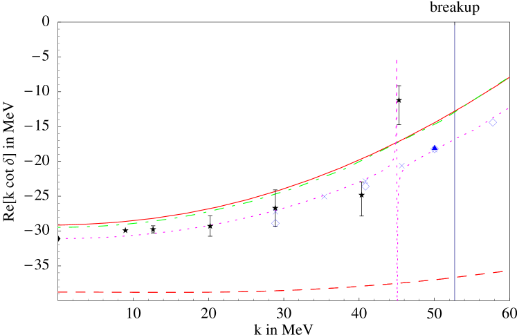
Figure 9: $k\cot\delta(k)$ vs. $k$ in the centre-of-mass frame below breakup and extraction of the quartet scattering length. The dashed line is the LO result, the solid (dot-dashed) line the NLO result with perturbative pions (pions integrated out). The dotted line is an NNLO calculation in effective field theory without pions [7]. The diamond at zero momentum is from the experiment of [38]. Stars denote the experiment by van Oers and Seagrave as reported in [33]. Results from realistic potential models are reported as squares from [34], crosses from [35] and triangles from [36].

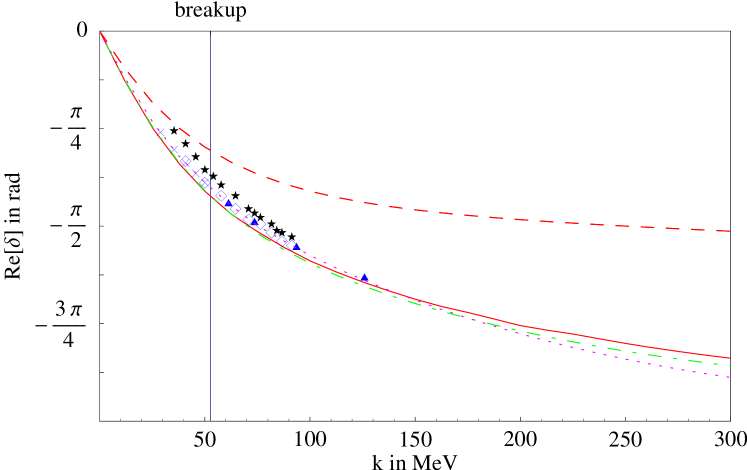
Figure 10: The real part of the phase shift above breakup. The stars are taken from the TUNL $pd$ phase shift analysis [34]. Remaining notation as in Fig. 9.

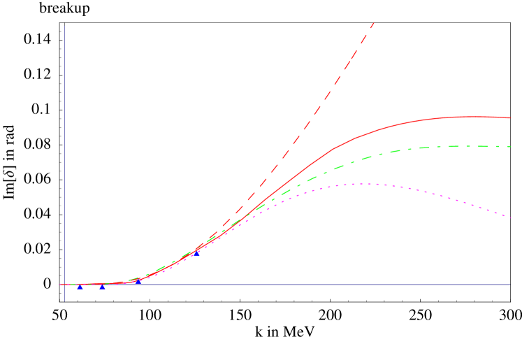
Figure 11: The imaginary part of the phase shift above breakup. Notation as in Fig. 9.

In Fig. 9, we focus on the behaviour below threshold where $p\ll m_{\pi}$. In this régime, the pions are expected to be integrated out resulting in a much simpler effective (“pion-less”) theory involving contact interactions between nucleons only [37, 6]. Besides our NLO result with explicit pions discussed above (full line), we also show the LO, NLO and NNLO calculation in a theory with pions integrated out (dashed, dash-dotted and dotted line). Simplistically, this is achieved by setting $g_{\mathrm{A}}=0$ in the determination of the parameters (2.2/2.18) and in the calculations of the NLO corrections. These calculations demonstrate convergence and predict a quartet scattering length in excellent agreement with experiment. The NLO calculation in the effective theory with and without pions give very similar results. The parameters in the pion-less and pion-full LO and NLO calculations were determined as described above to produce the physical values of $\gamma$ and $a^{{}^{3}S_{1}}$, while the NNLO result taken from [38, 6] used as input $a^{{}^{3}S_{1}}$ and the effective range $r_{0}=1.75\;\mathrm{fm}$, the difference of the two procedures to determine the parameters being of higher order in the power counting. No free parameters arise in any of the calculations.

The difference between the pion-full and pion-less theory should appear for momenta of the order of $m_{\pi}$ and higher because of non-analytical contributions of the pion cut. However, it is very moderate for momenta of up to $300\;\mathrm{MeV}$ in the centre-of-mass frame ($E_{\mathrm{cm}}\approx 70\;\mathrm{MeV}$), see Fig. 10. This and the lack of experimental data makes it difficult to assess whether the KSW power counting scheme to include pions as perturbative increases the range of validity over the pion-less theory . Unfortunately, numerical calculations with realistic potentials are not available for energies considerably higher than the deuteron breakup at the present time . Still, where data or numerical calculations are available, the pion-full theory does better than the pion-less one.

In deuteron calculations, the numerical value of the systematic expansion parameter $Q$ seems to be of the order $\frac{1}{3}$ at zero momentum, and we confirm this by comparing the quartet scattering length at LO and NLO: We find $a^{{}^{4}S_{\frac{3}{2}}}(\mathrm{LO})=(5.1\pm 1.5)\;\mathrm{fm}$, and at NLO with (without) perturbative pions $a^{{}^{4}S_{\frac{3}{2}}}(\mathrm{NLO,\pi})=(6.8\pm 0.7)\;\mathrm{fm}$ ($a^{{}^{4}S_{\frac{3}{2}}}(\mathrm{NLO,\mathrm{no}\,\pi})=(6.7\pm 0.7)\;\mathrm{fm}$). At NNLO,  [6] report $a^{{}^{4}S_{\frac{3}{2}}}(\mathrm{NNLO,\mathrm{no}\,\pi})=(6.33\pm 0.1)\;\mathrm{fm}$, and the experimental value is given in [38] as $a^{{}^{4}S_{\frac{3}{2}}}(\mathrm{exp})=(6.35\pm 0.02)\;\mathrm{fm}$. Comparing the NLO correction to the LO scattering length provides one with the error estimate quoted: The NLO calculation is estimated to be accurate up to about $(\frac{1}{3})^{2}\approx 10\%$. The NLO calculations with and without pions lie within each other’s error bar. The NNLO calculation quoted above is inside the error ascertained to the NLO calculation and carries itself an error of about $(\frac{1}{3})^{3}\approx 4\%$. NLO and LO contributions become comparable for momenta of more than $200\;\mathrm{MeV}$. In the imaginary part shown in Fig. 11, the same pattern emerges with a slightly more pronounced difference between the pion-less and pions-full theory.

Because results obtained with EFT are easily dissected for the relative importance of the various terms, we show that pionic corrections to $nd$ scattering in the quartet $\mathrm{S}$ wave channel – although formally NLO – are indeed much weaker: The calculation with perturbative pions and with pions integrated out do not differ significantly over a wide range of momenta.

Future work will extend the analysis presented here to higher partial waves and to the inclusion of Coulomb effects in order to allow for comparison with $pd$ data.

References

- [1] G.P. Lepage, “What Is Renormalization?,” Invited lectures given at TASI’89 Summer School, Boulder, CO, Jun 4-30, 1989, in: From Actions to Answers, T. DeGrand and D. Toussaint, eds., World Scientific 1990.
- [2] J. Gasser and H. Leutwyler, Ann. Phys. 158, 142 (1984).
- [3] S. Weinberg, Physica 96A, 327 (1979).
- [4] J. Gasser, M.E. Sainio and A. Svarc, Nucl. Phys. B307, 779 (1988).
- [5] E. Jenkins and A.V. Manohar, Phys. Lett. B255, 558 (1991).
- [6] P.F. Bedaque, H.W. Hammer and U. van Kolck, Phys. Rev. C58, R641 (1998), nucl-th/9802057; P.F. Bedaque and U. van Kolck, Phys. Lett. B428, 221 (1998), nucl-th/9710073.
- [7] P.F. Bedaque, H.W. Hammer and U. van Kolck, Phys. Rev. Lett. 82, 463 (1999), nucl-th/9809025; P.F. Bedaque, H.W. Hammer and U. van Kolck, Nucl. Phys. A646, 444 (1999), nucl-th/9811046; P.F. Bedaque, H.W. Hammer and U. van Kolck, nucl-th/9906032.
- [8] D.B. Kaplan, M.J. Savage and M.B. Wise, Phys. Lett. B424, 390 (1998), nucl-th/9801034; D.B. Kaplan, M.J. Savage and M.B. Wise, Nucl. Phys. B534, 329 (1998), nucl-th/9802075.
- [9] S. Weinberg, Nucl. Phys. B363, 3 (1991).
- [10] A.R. Levi, V. Lubicz and C. Rebbi, Phys. Rev. D56, 1101 (1997), hep-lat/9607022; A.R. Levi, V. Lubicz and C. Rebbi, Nucl. Phys. Proc. Suppl. 53, 275 (1997), hep-lat/9607025.
- [11] U. van Kolck, M. Savage and R. Seki, eds., “Nuclear Physics with Effective Field Theory”, Proceedings of the INT-Caltech Workshop (1999), World Scientific, in press.
- [12] T. Mehen and I.W. Stewart, nucl-th/9906010; S. Fleming, T. Mehen and I.W. Stewart, nucl-th/9906056; G. Rupak and N. Shoresh, nucl-th/9906077.
- [13] D.B. Kaplan, M.J. Savage and M.B. Wise, Phys. Rev. C59, 617 (1999), nucl-th/9804032.
- [14] J. Chen, H.W. Grießhammer, M.J. Savage and R.P. Springer, Nucl. Phys. A644, 221 (1998), nucl-th/9806080.
- [15] J. Chen, H.W. Grießhammer, M.J. Savage and R.P. Springer, Nucl. Phys. A644, 245 (1998), nucl-th/9809023.
- [16] D.B. Kaplan, M.J. Savage, R.P. Springer and M.B. Wise, Phys. Lett. B449, 1 (1999), nucl-th/9807081.
- [17] M.J. Savage, K.A. Scaldeferri and M.B. Wise, Nucl. Phys. A652, 273 (1999), nucl-th/9811029.
- [18] M.J. Savage and R.P. Springer, Nucl. Phys. A644, 235 (1998), nucl-th/9807014.
- [19] E. Epelbaum, Ulf-G. Mei ner, nucl-th/9902042, Phys. Lett. B, in press; E. Epelbaum, Ulf-G. Mei ner, nucl-th/9903046, to appear in the proceedings of Workshop on Nuclear Physics with Effective Field Theory: 1999, INT Seattle, Feb. 25-26, 1999.
- [20] T. Mehen and I.W. Stewart, Phys. Lett. B445, 378 (1999), nucl-th/9809071.
- [21] J. Gegelia, nucl-th/9805008.
- [22] H.W. Grießhammer, Phys. Rev. D58, 094027 (1998), hep-ph/9712467; H.W. Grießhammer, hep-ph/9810235 (to appear in Nucl. Phys. B).
- [23] T. Mehen and I.W. Stewart, nucl-th/9901064.
- [24] U. van Kolck, Nucl. Phys. A645, 273 (1999), nucl-th/9808007.
- [25] G. Rupak and N. Shoresh, nucl-th/9902077.
- [26] V.G.J. Stoks, R.A.M. Klomp, C.P.F. Terheggen and J.J. de Swart, Phys. Rev. C49, 2950 (1994), nucl-th/9406039.
- [27] G.V. Skornyakov and K.A. Ter-Martirosian, Sov. Phys. JETP 4 (1957) 648.
- [28] J.H. Hetherington and L.H. Schick, Phys. Rev. B137, 935 (1965); R.T. Cahill and I.H. Sloan, Nucl. Phys. A165, 161 (1971).
- [29] R. Aaron and R.D. Amado, Phys. Rev. 150, 857 (1966).
- [30] E.W. Schmid and H. Ziegelmann, The Quantum Mechanical Three-Body Problem, Vieweg Tracts in Pure and Applied Physics Vol. 2, Pergamon Press (1974).
- [31] D.D. Brayshaw, Phys. Rev. 176, 1855 (1968).
- [32] G. S. Danilov and V. I. Lebedev, Sov. Phys. JETP 17 (1963) 1015.
- [33] A.C. Phillips and G. Barton, Phys. Lett. B28, 376 (1969).
- [34] W. Tornow and H. Witała, “Proton-Deuteron Phase-Shift Analysis Above the Deuteron Breakup Threshold”, Technical Report TUNL XXXVI (1996-97).
- [35] A. Kievsky, S. Rosati, W. Tornow and M. Viviani, Nucl. Phys. A607, 402 (1996).
- [36] D. Hüber, J. Golak, H. Witała, W. Glöckle and H. Kamada, “Phase Shift and Mixing Parameters for Elastic Scattering above the Breakup Threshold”.
- [37] J. Chen, G. Rupak and M.J. Savage, nucl-th/9902056.
- [38] W. Dilg, L. Koester and W. Nistler, Phys. Lett. B36, 208 (1971).