The Anapole Form Factor of the Deuteron

Abstract

We find the leading order result for the anapole form factor of the deuteron using effective field theory. The momentum dependence of the anapole form factor is different from that of the matrix element of the strange currents in the deuteron, which may provide a way for disentangling these two competing effects when analyzing parity violating electron-deuteron scattering experiments. We give closed form expressions for both the form factor and integrals often encountered in the NN effective field theory.

I Introduction

Several open questions in nuclear parity violation[1, 2] prompt further investigation of parity violating observables in the simplest nuclear system. Recently, a precise measurement of the parity violating angular asymmetry in $\overrightarrow{n}p\rightarrow d\gamma$ was proposed[3] in order to tightly constrain the weak one-pion-nucleon coupling constant, $h_{\pi NN}^{(1)}$. In addition, MIT-Bates has a dedicated program to measure parity violation in electron scattering on the deuteron[4], which depends upon both the strangeness content of the deuteron, and on weak nonleptonic interactions which generate an anapole interaction. Both measurements will constrain $h_{\pi NN}^{(1)}$, free from finite density effects that contaminate extractions from measurements in light and heavy nuclei.

For low momentum scattering, an effective field theory treatment[5, 6, 7, 8, 9, 10, 11, 12, 13, 14, 15, 16, 17, 18, 19, 20, 21, 22, 23, 24, 25, 26, 27] of the deuteron is both systematic and predictive[10, 25]. The language and notation used in this paper is based upon refs.[9] and [26]. Here we generalize the calculation of the deuteron anapole moment[26] by retaining the dependence upon the momentum transfer from the virtual photon, thereby determining the full anapole form factor at leading order (LO) in the effective field theory expansion.

If sufficient data can be taken at $Q^{2}$ low enough for the effective field theory to be valid, the momentum dependence of the parity violation from electron scattering on the deuteron should follow, up to higher order corrections, the form we obtain. In that case, it may be possible to extract not only the strange axial matrix element of the nucleon, but also the (presently controversial) value of the parity violating pion-nucleon coupling.

II Effective Lagrangian

We give here the effective Lagrangian needed for this calculation[9, 26]. A discussion of the power counting used to determine the order at which each diagram contributes is presented there. Both strong and weak interactions are required for the leading order anapole form factor.

The strong interactions of the pions and nucleons are described by

$${\cal L}_{strong} = {f^{2}\over 8}TrD_{\mu}\Sigma D^{\mu}\Sigma^{\dagger}+N^{\dagger}\left(iD_{0}+{{\bf D}^{2}\over 2M_{N}}\right)N+{ig_{A}\over 2}N^{\dagger}{\bf\sigma}\cdot(\xi{\bf D}\xi^{\dagger}-\xi^{\dagger}{\bf D}\xi)N$$ (1)

$$+ {e\over 2M_{N}}N^{\dagger}(\kappa_{0}+\kappa_{1}\tau_{3})\sigma\cdot{\bf B}N-C^{({}^{3}\kern-0.98ptS_{1})}_{0}(N^{T}P_{i,0}N)^{\dagger}(N^{T}P_{i,0}N)\ +\ \cdots\ \ \ ,$$ (2)

where the pion fields are contained in a special unitary matrix,

$$\Sigma=\xi^{2}=\exp{2i\Pi\over f},\qquad\Pi=\left(\begin{array}[]{cc}\pi^{0}/\sqrt{2}&\pi^{+}\\ \pi^{-}&-\pi^{0}/\sqrt{2}\end{array}\right),$$ (3)

with $f=132\ {\rm\ MeV}$. $N$ is the isospin doublet of nucleon fields, $M_{N}$ is the nucleon mass, $g_{A}~{}\sim~{}1.25$ is the axial coupling constant, $D^{\mu}$ is the covariant derivative, and the ellipses represent operators involving more insertions of the light quark mass matrix, meson fields, and spatial derivatives. The isoscalar and isovector magnetic moments are $\kappa_{0}=0.44$ and $\kappa_{1}=2.35$ in units of nuclear magnetons. $P_{i,0}$ is the spin-isospin projector for the ${}^{3}\kern-1.4ptS_{1}$ channel, defined by

$$P_{i,0} \equiv {1\over\sqrt{8}}\sigma_{2}\sigma_{i}\ \tau_{2}\ ,\qquad{\rm Tr\,}P_{i,0}^{\dagger}P_{j,0}={1\over 2}\delta_{ij}\ ,$$ (4)

The coefficient $C_{0}^{({}^{3}\kern-0.98ptS_{1})}=-5.51{\rm\ fm}^{2}$ has been determined from fits to the S-wave phase shifts in the ${}^{3}\kern-1.4ptS_{1}$ channels [9], renormalized at $\mu=m_{\pi}$ in the power divergence subtraction scheme (PDS)[9].

The leading order weak interaction Lagrange density is

$${\cal L}^{\Delta I=1}_{\rm weak} = i\ h_{\pi NN}^{(1)}\ \pi^{+}\ p^{\dagger}n\ +\ {\rm h.c.}\ +\cdots$$ (5)

where the ellipses represent higher order terms in the chiral and momentum expansion.

The value of the parity violating pion-nucleon coupling, $h_{\pi NN}^{(1)}$, is controversial. Theoretical treatments provide qualitative ranges, but experimental results are in disagreement[1, 2, 28, 29]. However, if we take the generally accepted size of $h_{\pi NN}^{(1)}\sim 10^{-7}$ [30, 31, 32, 33, 34, 35], then $h_{\pi NN}^{(1)}$ is responsible for the leading order parity violating effects in the deuteron. Strong interaction effects in the deuteron are dominated by $C_{0}^{({}^{3}\kern-0.98ptS_{1})}$, with higher order corrections coming from pion exchange and contact terms multiplying operators with two derivatives or quark mass insertions. In the KSW power counting (outlined in [9]), strong interaction pions are treated in perturbation theory, and are sub-leading compared to the four-nucleon contact interactions. In the calculations of deuteron observables and interactions that have been computed with KSW power counting, there are no indications that the pionic contributions are larger than naively expected. Calculations at next-to-next-to leading order (NNLO) (for recent progress in this area see [36, 37]) will allow more definite conclusions about the convergence of the theory to be made[38].

III The Anapole Form Factor of the Deuteron

The anapole form factor of the deuteron, $A_{D}(|{\bf k}|)$, describes its spin-dependent coupling to the electromagnetic field for arbitrary momentum transfer, defined through

$${\cal L} = iA_{D}(|{\bf k}|)\ {1\over M_{N}^{2}}\ \epsilon_{abc}D^{a\dagger}D^{b}\partial_{\mu}F^{\mu c}\ \ \ ,$$ (6)

where ${\bf k}$ is the three momentum of the photon, $F^{\mu c}$ is the electromagnetic field strength tensor, and $i\epsilon_{abc}D^{a\dagger}D^{b}$ is the deuteron spin operator. The equations of motion for the electromagnetic field allow this interaction to be written in terms of local four-fermion interactions, and therefore this does not correspond to a coupling between a nucleon and an on-shell photon.

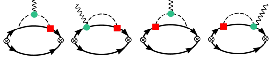
FIG. 1.: Leading order diagrams contributing to the deuteron anapole form factor. These are the single nucleon contributions, written as $A_{N}(|{\bf k}|)$ in the text. The crossed circles represent operators that create or annihilate two nucleons with the quantum numbers of the deuteron. The solid square is the weak operator with coefficient $h^{(1)}_{\pi NN}$, and the solid circle is the minimal coupling to the electromagnetic field. Wavy lines are photons, solid lines are nucleons, and dashed lines are mesons.

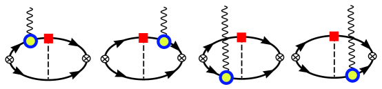
FIG. 2.: Leading order diagrams contributing to the deuteron anapole form factor. These are the magnetic coupling contributions, written as $A_{M}(|{\bf k}|)$ in the text. The crossed circles represent operators that create or annihilate two nucleons with the quantum numbers of the deuteron. The solid square is the weak operator with coefficient $h^{(1)}_{\pi NN}$, and the open circle is the magnetic coupling to the electromagnetic field. Wavy lines are photons, solid lines are nucleons, and dashed lines are mesons.

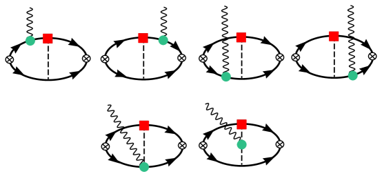
FIG. 3.: Leading order diagrams contributing to the deuteron anapole form factor. These are electric coupling contributions, written as $A_{E}(|{\bf k}|)$ in the text. The crossed circles represent operators that create or annihilate two nucleons with the quantum numbers of the deuteron. The solid square is the weak operator with coefficient $h^{(1)}_{\pi NN}$, and the solid circle is the minimal coupling to the electromagnetic field. Wavy lines are photons, solid lines are nucleons, and dashed lines are mesons.

The anapole form factor, $A_{D}(|{\bf k}|)$, is separated into three parts: the single nucleon contribution $A_{N}$, the magnetic contribution $A_{M}$, and the electric contribution $A_{E}$, with

$$A_{D}(|{\bf k}|)=A_{N}(|{\bf k}|)+A_{M}(|{\bf k}|)+A_{E}(|{\bf k}|)\ \ .$$ (7)

The expressions we obtain for the form factors use methods outlined in ref. [27]. While the regularization and renormalization prescription used in [27] does not directly lead to gauge invariant results, by matching orders in a $|{\bf k}|^{2}$ expansion to known dimensionally regularized results, we can recover the full dimensionally regulated expression. In the appendix we show individual integrals which are relevant for this calculation (as well as other two loop pion exchange calculations).

The diagrams in fig. (1) that constitute the contribution from the single nucleon factorize into the product of the single nucleon anapole form factor (generated by $h_{\pi NN}^{(1)}$, see [39]) with the LO deuteron charge form factor to yield

$$A_{N}(|{\bf k}|)=-{g_{A}eh_{\pi NN}^{(1)}M_{N}^{2}\over\pi f}{2\gamma\over|{\bf k}|^{4}}\left[(m_{\pi}^{2}+{|{\bf k}|^{2}\over 4})\ \tan^{-1}\left({|{\bf k}|\over 2m_{\pi}}\right)-{m_{\pi}|{\bf k}|\over 2}\right]\tan^{-1}\left({|{\bf k}|\over 4\gamma}\right)\ \ ,$$ (8)

where $\gamma=\sqrt{M_{N}B}$ is the binding momentum of the deuteron with $B$ the deuteron binding energy.

The magnetic contribution, arising from the interaction of the electromagnetic field with the isovector magnetic moment of the nucleon, comes from the diagrams shown in fig. (2).

$$A_{M}(|{\bf k}|) = -{g_{A}eh_{\pi NN}^{(1)}M_{N}^{2}\over 2\pi f}{\kappa_{1}\over|{\bf k}|^{2}}\left[2\gamma-m_{\pi}+{m^{2}_{\pi}\over 2\gamma}{\log\left[{(m_{\pi}+2\gamma)^{2}\over(m_{\pi}+2\gamma)^{2}+{|{\bf k}|^{2}\over 4}}\right]}\right.$$ (13)

$$+\ {|{\bf k}|\over 4\gamma^{2}}\left(m^{2}_{\pi}\log\left[1+{2\gamma\over m_{\pi}}\right]+2\gamma^{2}-2\gamma m_{\pi}\right){\tan^{-1}\left({|{\bf k}|\over 4\gamma}\right)}\$$

$$\ +\ \left(-{8\gamma^{2}\over|{\bf k}|}-{|{\bf k}|\over 2}+{|{\bf k}|m_{\pi}\over 2\gamma}+{2m^{2}_{\pi}\over|{\bf k}|}\right){\tan^{-1}\left({|{\bf k}|\over 2(m_{\pi}+2\gamma)}\right)}$$

$$+\ \ i{m^{2}_{\pi}|{\bf k}|\over 8\gamma^{2}}\left.\left(Li_{2}\left({-i|{\bf k}|\over 2(m_{\pi}+2\gamma)}\right)-Li_{2}\left({i|{\bf k}|\over 2(m_{\pi}+2\gamma)}\right)\right.\right.$$

$$\left.\left.\qquad\qquad\qquad-Li_{2}\left({-i|{\bf k}|-4\gamma\over 2m_{\pi}}\right)+Li_{2}\left({i|{\bf k}|-4\gamma\over 2m_{\pi}}\right)\ \right)\right]\ \ ,$$

where $Li_{2}(z)$ is the dilogarithm function, given in the appendix.

The electric contribution, arising from the minimal coupling of the electromagnetic field to pions and non-relativistic nucleons, comes from the diagrams shown in fig. (3).

$$A_{E}(|{\bf k}|) = -{g_{A}eh_{\pi NN}^{(1)}M_{N}^{2}\over 8\pi f}\ {1\over|{\bf k}|}\left\{-m_{\pi}|{\bf k}|-{(m_{\pi}-\gamma)(|{\bf k}|^{2}+16\gamma^{2})\over 2\gamma}\tan^{-1}\left({|{\bf k}|\over 4\gamma}\right)\right.$$ (22)

$$\left.+{|{\bf k}|^{2}(m_{\pi}-\gamma)+4\gamma(m_{\pi}^{2}-4\gamma^{2})\over 2\gamma}\tan^{-1}\left({|{\bf k}|\over 2(m_{\pi}+2\gamma)}\right)\right.$$

$$\left.-{|{\bf k}|m_{\pi}^{2}\over 2\gamma}\log\left[{{|{\bf k}|^{2}\over 4}+(m_{\pi}+2\gamma)^{2}\over(m_{\pi}+2\gamma)^{2}}\right]\ +\ {m_{\pi}^{2}(|{\bf k}|^{2}+16\gamma^{2})\over 4\gamma^{2}}\tan^{-1}\left({|{\bf k}|\over 4\gamma}\right)\log\left[1+{2\gamma\over m_{\pi}}\right]\right.$$

$$\left.-2\gamma\rho\tan^{-1}\left({|{\bf k}|\over 2m_{\pi}+\rho}\right)\log\left[{|{\bf k}|^{2}+4(m_{\pi}+2\gamma)^{2}\over(\rho+4\gamma)^{2}}\right]\right.$$

$$\left.+2\gamma\rho\tan^{-1}\left({|{\bf k}|\over 2(m_{\pi}+2\gamma)}\right)\log\left[{(\rho-4\gamma)^{2}\over 2\rho(\rho+2m_{\pi})}\right]\right.$$

$$\left.+i{m_{\pi}^{2}(|{\bf k}|^{2}+16\gamma^{2})\over 8\gamma^{2}}\left[Li_{2}\left({i|{\bf k}|-4\gamma\over 2m_{\pi}}\right)-Li_{2}\left({-i|{\bf k}|-4\gamma\over 2m_{\pi}}\right)\right.\right.$$

$$\left.\left.\qquad\qquad\qquad\qquad+Li_{2}\left({-i|{\bf k}|\over 2(m_{\pi}+2\gamma)}\right)-Li_{2}\left({i|{\bf k}|\over 2(m_{\pi}+2\gamma)}\right)\right]\right.$$

$$\left.+i2\gamma\rho\left[Li_{2}\left({-i|{\bf k}|-2m_{\pi}-4\gamma\over\rho-4\gamma}\right)-Li_{2}\left({i|{\bf k}|-2m_{\pi}-4\gamma\over\rho-4\gamma}\right)\right.\right.$$

$$\left.\left.\qquad\qquad+Li_{2}\left({-i|{\bf k}|+\rho-2m_{\pi}\over\rho+4\gamma}\right)-Li_{2}\left({i|{\bf k}|+\rho-2m_{\pi}\over\rho+4\gamma}\right)\right]\ \ \right\}\ \ ,$$

where $\rho=\sqrt{|{\bf k}|^{2}+4m^{2}_{\pi}}$.

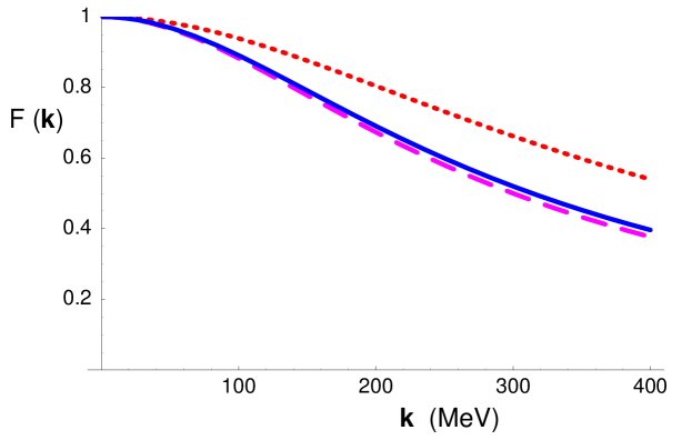
FIG. 4.: The three contributions to the anapole form factor as a function of momentum transfer $|{\bf k}|$, each normalized to unity at $|{\bf k}|=0$. The solid curve corresponds to the contribution from the single nucleon anapole form factor, $\tilde{A}_{N}(|{\bf k}|)$ (see fig. (1)). The dashed curve shows the contribution from the photon coupling to the isovector nucleon magnetic moment, $\tilde{A}_{M}(|{\bf k}|)$ (see fig. (2)). The dotted curve corresponds to the electric form factor, $\tilde{A}_{E}(|{\bf k}|)$ (see fig. (3)).

IV Discussion of Results

For illustrative purposes, we explicitly factor out the normalization of each of the form factors contributing to the anapole moment of the deuteron. The normalized single nucleon, magnetic, and electric form factors, $\tilde{A}_{N}$, $\tilde{A}_{M}$, and $\tilde{A}_{E}$ respectively, are defined through

$$A_{D}(|{\bf k}|) = -{eg_{A}h_{\pi NN}^{(1)}M_{N}^{2}\over 12\pi f}\left[\ {1\over 2m_{\pi}}\tilde{A}_{N}(|{\bf k}|)\ +\ \kappa_{1}\ {m_{\pi}+\gamma\over(m_{\pi}+2\gamma)^{2}}\ \tilde{A}_{M}(|{\bf k}|)\right.$$ (24)

$$\left.\qquad\qquad\qquad\qquad\ -\ {m_{\pi}^{2}+3m_{\pi}\gamma+12\gamma^{2}\over 6m_{\pi}(m_{\pi}+2\gamma)^{2}}\tilde{A}_{E}(|{\bf k}|)\ \ \right]$$

$$= -{eg_{A}h_{\pi NN}^{(1)}M_{N}^{2}\over 12\pi f}\left[\ {1\over 2m_{\pi}}\ +\ \kappa_{1}\ {m_{\pi}+\gamma\over(m_{\pi}+2\gamma)^{2}}\ -{m_{\pi}^{2}+3m_{\pi}\gamma+12\gamma^{2}\over 6m_{\pi}(m_{\pi}+2\gamma)^{2}}\right]\tilde{A}_{D}(|{\bf k}|)\ \ \ ,$$ (25)

where $\tilde{A}_{M}(0)\ =\ \tilde{A}_{N}(0)\ =\ \tilde{A}_{E}(0)\ =\ 1$. The deuteron anapole form factor, $\tilde{A}_{D}(|{\bf k}|)$, is normalized so that $\tilde{A}_{D}(0)=1$. (Note that while $A_{D}=A_{N}+A_{M}+A_{E}$, the normalized $\tilde{A}_{D}$ does not equal the sum of the individual tilded form factors.)

Fig. (4) shows that at LO in the effective field theory expansion the form factor associated with the single nucleon and magnetic contributions fall somewhat faster than the contribution from the electric form factor, versus increasing momentum transfer. The power counting for this effective field theory [9] suggests that corrections to the LO result are naively at the 30% level. While it is possible that the differences between the form factors computed at LO are modified by higher order contributions, there is no reason for the form factors to be identical.

The anapole form factor of the deuteron contributes to parity violation in electron scattering off the deuteron. A simultaneous source of parity violation in such an experiment is provided by any intrinsic strangeness existing in the deuteron. In a previous calculation [26], we gave an expression for the leading order parity violating matrix element in electron-deuteron scattering in terms of the deuteron anapole moment and the strange axial matrix element of the nucleon. The present calculation extends this work, and increases the possibility of separating the two effects, by generalizing the moment to the momentum dependent form factor. To do this we need to estimate how the strange axial matrix element depends on momentum transfer.

The scale for the variation of the anapole form factors is set by the deuteron binding momentum, $\gamma$, and the pion mass. In contrast, the variation of the form factors describing the matrix element of the strange axial current is set by the deuteron binding momentum, and the kaon mass or some higher mass scale. Therefore, we expect the contribution to parity violating electron-deuteron scattering from the matrix element of the axial strange quark current to become more important at higher momentum transfers. The fall of the strange quark form factor with momentum should be driven by the small deuteron binding energy; that is, by the nucleon recoil effects. This gives the LO strange deuteron form factor the same structure as the LO deuteron charge form factor,

$$F_{C}(|{\bf k}|) = {4\gamma\over|{\bf k}|}\tan^{-1}\left({|{\bf k}|\over 4\gamma}\right)\ \ \ .$$ (26)

The parity violating amplitude in electron-deuteron scattering is then, at LO in the effective field theory,

$${\cal A}^{(pv)}(|{\bf k}|) = 10^{-7}\left(5.4\ g_{\Delta S}\ F_{C}(|{\bf k}|)\ -\ 0.21\left({h^{(1)}_{\pi NN}\over 10^{-7}}\right)\tilde{A}_{D}(|{\bf k}|)\right){1\over M_{N}^{2}}\ \epsilon^{abi}\ \overline{e}\gamma_{i}e\ \varepsilon^{*}_{a}\ \varepsilon_{b}\ \ \ .$$ (27)

The two contributions to the anapole form factor are shown in fig. (5).

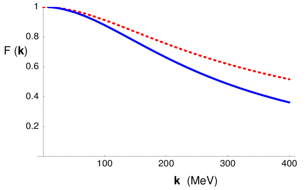
FIG. 5.: A comparison between the normalized anapole form factor, $\tilde{A}_{D}(|{\bf k}|)$ defined in eq. (25), and the charge form factor, expected to describe the matrix element of the strange axial current at LO. The solid curve is the anapole form factor while the dotted curve corresponds to the charge form factor $F_{C}(|{\bf k}|)$.

A more precise estimate of the form factors, and hence a more precise estimate of $h_{\pi NN}^{(1)}$ through a comparison with electron-deuteron scattering data, would require a higher order calculation of the anapole form factor in addition to more insight into possible strange quark effects (while current measurements of $g_{\Delta s}$ are consistent with zero[40, 41, 42], so is one of the measurements of $h_{\pi NN}^{(1)}$[28].) An estimate of the size of the higher order corrections entering at NLO and higher can be made by examining the size of the corrections to the charge form factor, as presented in [10]. Compact, analytic expressions for the LO form factors have been obtained in this work, and it is likely that similarly simple expressions can be obtained at NLO.

It is appropriate to comment on the recent work by Khriplovich and Korkin[43] who determine the anapole moment of the deuteron in the zero-range potential limit. They find (using their revised expression for the magnetic moment term) a contribution from the electric and magnetic interactions (not including the single nucleon contribution) proportional to

$$A_{D}^{(KK)} \propto {m_{\pi}+\gamma\over(m_{\pi}+2\gamma)^{2}}\left(\kappa_{1}-{1\over 6}\right)\ \ \ .$$ (28)

The expression we obtained in [26] does not reproduce their result, except in the limiting case where $\gamma\rightarrow 0$. It is clear that their expression, shown in eq. (28), does not have the correct behavior in the chiral limit for fixed $\gamma$ (the deuteron anapole moment would diverge, driven by the single nucleon contribution), as discussed in [26]. The deuteron anapole moment cannot have any $1/m_{\pi}$ dependence in the chiral limit when $\gamma$ is held fixed, due to the vanishing of the strong one-pion-deuteron coupling. Our result, shown in eq. (25), correctly reproduces this necessary behavior.

V Conclusion

In this work we have presented an analytic expression for the anapole form factor at LO in the effective field theory expansion. The dominant contribution to this form factor is from pion physics, through the weak pion-nucleon coupling $h_{\pi NN}^{(1)}$. The pion mass and deuteron binding momentum are the scales that drive its variation. In contrast, pion effects will not dominate the matrix element of the strange axial current. We find that while the deuteron binding momentum provides most of the momentum variation of both form factors, the anapole form factor falls fasters than the matrix element of the strange axial current. This has important implications for the determination of both $g_{\Delta s}$ and $h_{\pi NN}^{(1)}$ from parity violating electron-deuteron scattering. Encouraged by the success of effective field theory for this parity violating process, and the relatively simple closed form expressions we obtain, we are optimistic about higher order calculations of this form factor and the possibilities of extracting $h_{\pi NN}^{(1)}$ from electron scattering experiments.

This work is supported in part by the U.S. Dept. of Energy under Grants No. DE-FG03-97ER4014 and DE-FG02-96ER40945, and NSF grant number 9870475.

VI Appendix of Integrals

The analytic expressions we found for the anapole form factors come from integrals which are relevant for other calculations. In this appendix we give expressions for the general form of some of the integrals encountered in evaluating the Feynman diagrams for the anapole calculation. We use a combination of dimensional regularization and the position space representation (as advocated by Binger[27]) to find expressions for the integrals. The divergent contribution and well defined finite piece will be given in terms of

$$\Gamma = \Gamma[4-n]\ +\log\left(\pi\right)\ +\ 1\ \ \ ,$$ (29)

where $n$ is the number of space-time dimensions. To be consistent with the PDS procedure, $\mu/2$ and not $\mu$ is used for the dimensional regularization mass-scale in the definition of the integrals. In the expressions that follow, the magnitude of the three-momentum transfer is given by $k=|{\bf k}|$. All integrals have been power-series expanded about $n=4$, so terms of order $(n-4)^{1}$ or higher are not shown. Where needed to distinguish one integral from another within a class (same denominators in the integrand), a subscript is used to indicate the naive degree of ultraviolet divergence of the diagram.

A 1-Loop, 2-Propagators

We find that two-loop integrals often reduce down to some simple functions, dilogarithms, and the following integral (which also appears in one loop diagrams):

$$A(a,b;k) = \int{d^{3}{\bf q}\over(2\pi)^{3}}{1\over[({\bf q}-{1\over 2}{\bf k})^{2}+a^{2}]}{1\over[{\bf q}^{2}+b^{2}]}\ =\ {1\over 2\pi k}\tan^{-1}\left({k\over 2(a+b)}\right)\ \ \ .$$ (30)

B 2-Loops, 3-Propagators

A frequently encountered integral in the theory with perturbative pions[8, 9] is $B_{0}(a,b,c;\mu;k)$ evaluated at $k=0$ (an integral that is ultra-violet divergent as $n\rightarrow 4$) where

$$B_{0}(a,b, c;\mu;k)$$ (32)

$$=\left({\mu\over 2}\right)^{8-2n}\int{d^{n-1}{\bf q}\over(2\pi)^{n-1}}{d^{n-1}{\bf l}\over(2\pi)^{n-1}}\ {1\over[({\bf q}-{1\over 2}{\bf k})^{2}+a^{2}]}{1\over[({\bf q}+{\bf l})^{2}+b^{2}]}{1\over[{\bf l}^{2}+c^{2}]}\ \ \ .$$

It can be computed at $k=0$ using dimensional regularization:

$$B_{0}(a,b,c;\mu;0) = -{1\over(4\pi)^{n-1}}\ \Gamma[4-n]\ \Gamma[{3-n\over 2}]\ \Gamma[{n-3\over 2}]\ \left({2M\over\mu}\right)^{2n-8}$$ (33)

$$= {1\over 32\pi^{2}}\left[\Gamma-2\log\left[{M\over\mu}\right]\ \ \right]\ \ \ ,$$ (34)

where $M=a+b+c$. The methods of [27] are used to find the finite $k$-dependent portion, which matches onto the previous result to give the full expression for arbitrary $k$:

$$B_{0}(a,b,c;\mu;k) = {1\over 32\pi^{2}}\left[\ \Gamma-\log\left[{M^{2}+{k^{2}\over 4}\over\mu^{2}}\right]-{4M\over k}\tan^{-1}\left({k\over 2M}\right)+2\ \right]\ \ \ .$$ (35)

This reduces to eq. (34) in the limit $k\rightarrow 0$, as required.

A related integral is

$$B_{1}(a,b,c;\mu;k) = \left({\mu\over 2}\right)^{8-2n}\int{d^{n-1}{\bf q}\over(2\pi)^{n-1}}{d^{n-1}{\bf l}\over(2\pi)^{n-1}}\ {{\bf q}\cdot{\bf k}\over[({\bf q}-{1\over 2}{\bf k})^{2}+a^{2}]}{1\over[({\bf q}+{\bf l})^{2}+b^{2}]}{1\over[{\bf l}^{2}+c^{2}]}\ .$$ (36)

Making the replacement ${\bf q}\cdot{\bf k}\rightarrow-({\bf q}-{1\over 2}{\bf k})^{2}+{\bf q}^{2}+{1\over 4}{\bf k}^{2}$ leaves a more divergent integral (the ${\bf q}^{2}$ term) than found in the $B_{0}$ integral, but a judicious combination of terms allows explicit evaluation of this integral using the methods of [27]. We find

$$B_{1}(a,b,c;\mu;k)={1\over 32\pi^{2}} \left[\ {k^{2}\over 3}\left(\Gamma+2-\log\left[{M^{2}+{k^{2}\over 4}\over\mu^{2}}\right]\right)\ +\ 2aM-\ {2\over 3}M^{2}\right.$$ (38)

$$\left.-\ \left({4a\over k}M^{2}+Mk-{4\over 3k}M^{3}+ak\right)\tan^{-1}\left({k\over 2M}\right)\right]\ \ \ .$$

C 2-Loops, 4-Propagators

In graphs where an external current couples to a nucleon line and a perturbative pion is exchanged between nucleons, we encounter integrals with four propagators and two loop momentum integrations. Such integrals are expressed in terms of simple functions and dilogarithmic functions. The function $P(X,Y;k)$ is defined to be

$$P(X,Y;k) = \int_{-1}^{+1}\ dz\ {\log\left[X+i{kz\over 2}\right]\over Y+i{kz\over 2}}$$ (39)

$$= -i{2\over k}\left\{Li_{2}\left[{X+i{k\over 2}+i\epsilon\over X-Y+i\epsilon}\right]\ -\ Li_{2}\left[{X-i{k\over 2}-i\epsilon\over X-Y-i\epsilon}\right]\right.$$ (43)

$$+i2\pi\log\left[X-Y+i\epsilon\right]\ \theta\left[X-Y\right]\theta\left[Y\right]$$

$$+\log\left[X+i{k\over 2}+i\epsilon\right]\log\left[{Y+i{k\over 2}+i\epsilon\over Y-X+i\epsilon}\right]$$

$$\left.-\log\left[X-i{k\over 2}-i\epsilon\right]\log\left[{Y-i{k\over 2}-i\epsilon\over Y-X-i\epsilon}\right]\ \right\}\ \ \ ,$$

where the dilogarithmic function $Li_{2}(z)$ is conventionally defined

$$Li_{2}(z) = -\int_{0}^{z}\ dt\ {\log[1-t]\over t}\ =\ \int_{0}^{1}\ dx\ {\log[x]\over x-{1\over z}}\ \ \ .$$ (44)

The simplest integral involving four propagators at two loops does not have any loop momentum dependence in the numerator, and is finite at $n=4$. It is expressed in terms of functions defined previously,

$$I_{-2}(a,b,c,d;k)\ =\ \int{d^{3}{\bf q}\over(2\pi)^{3}}{d^{3}{\bf l}\over(2\pi)^{3}}\ {1\over[({\bf q}-{1\over 2}{\bf k})^{2}+a^{2}]}{1\over[{\bf q}^{2}+b^{2}]}{1\over[({\bf q}+{\bf l})^{2}+c^{2}]}{1\over[{\bf l}^{2}+d^{2}]}$$ (45)

$$={1\over 64\pi^{2}b}\left\{\phantom{{k\over k}}P(a+c+d,a-b;k)-P(a+c+d,a+b;k)\right.$$ (46)

$$\left.\quad+i{2\over k}\log\left(b+c+d\right)\left[\log\left(a-b+i{k\over 2}+i\epsilon\right)-\log\left(a-b-i{k\over 2}-i\epsilon\right)-i2\pi\theta(b-a)\right.\right.$$ (47)

$$\left.\left.\qquad\qquad\qquad\qquad\qquad-\log\left(a+b+i{k\over 2}+i\epsilon\right)+\log\left(a+b-i{k\over 2}-i\epsilon\right)\right]\ \right\}\ \ \ .$$ (48)

An integral with a more complicated momentum dependence, but without Lorentz structure in the numerator of the integrand, can be written in terms of $I_{-2}$,

$$\tilde{I}_{-2}(a,b,c,d;k) = \int{d^{3}{\bf q}\over(2\pi)^{3}}{d^{3}{\bf l}\over(2\pi)^{3}}\ {1\over[({\bf q}-{1\over 2}{\bf k})^{2}+a^{2}]}{1\over[({\bf q}+{1\over 2}{\bf k})^{2}+b^{2}]}{1\over[({\bf q}+{\bf l})^{2}+c^{2}]}{1\over[{\bf l}^{2}+d^{2}]}$$ (49)

$$= {1\over 2}\left[I_{-2}(a,\sqrt{{k^{2}\over 4}+{a^{2}\over 2}+{b^{2}\over 2}},c,d)\ +\ I_{-2}(b,\sqrt{{k^{2}\over 4}+{a^{2}\over 2}+{b^{2}\over 2}},c,d)\right]\ \ \ .$$ (50)

We will use the following integrals in subsequent expressions.

$$I_{-1}(a,b,c,d;k) = \int{d^{3}{\bf q}\over(2\pi)^{3}}{d^{3}{\bf l}\over(2\pi)^{3}}{{\bf q}\cdot{\bf k}\over[({\bf q}-{1\over 2}{\bf k})^{2}+a^{2}]}{1\over[{\bf q}^{2}+b^{2}]}{1\over[({\bf q}+{\bf l})^{2}+c^{2}]}{1\over[{\bf l}^{2}+d^{2}]}$$ (51)

$$= B_{0}(a,c,d;\mu;k)-B_{0}(b,c,d;\mu;0)-(b^{2}-a^{2}-{k^{2}\over 4})I_{-2}(a,b,c,d;k)\ \ \ ,$$ (52)

$$I_{0}(a,b,c ,d;\mu;k)$$ (56)

$$=\left({\mu\over 2}\right)^{8-2n}\int{d^{n-1}{\bf q}\over(2\pi)^{n-1}}{d^{n-1}{\bf l}\over(2\pi)^{n-1}}\ {\left({\bf q}\cdot{\bf k}\right)^{2}\over[({\bf q}-{1\over 2}{\bf k})^{2}+a^{2}]}{1\over[{\bf q}^{2}+b^{2}]}{1\over[({\bf q}+{\bf l})^{2}+c^{2}]}{1\over[{\bf l}^{2}+d^{2}]}$$

$$=B_{1}(a,c,d;\mu;k)+(b^{2}-a^{2}-{k^{2}\over 4})\ \left(B_{0}(b,c,d;\mu;0)-B_{0}(a,c,d;\mu;k)\right)$$

$$\ \ +(b^{2}-a^{2}-{k^{2}\over 4})^{2}\ I_{-2}(a,b,c,d;k)\ \ \ .$$

The first integral with a Lorentz index, but finite at $n=4$, is

$$J_{-1}^{j}(a,b, c,d;k)=\int{d^{3}{\bf q}\over(2\pi)^{3}}{d^{3}{\bf l}\over(2\pi)^{3}}{{\bf l}^{j}\over[({\bf q}-{1\over 2}{\bf k})^{2}+a^{2}]}{1\over[{\bf q}^{2}+b^{2}]}{1\over[({\bf q}+{\bf l})^{2}+c^{2}]}{1\over[{\bf l}^{2}+d^{2}]}$$ (58)

$$={{\bf k}^{j}\over{\bf k}^{2}}\int{d^{3}{\bf q}\over(2\pi)^{3}}{d^{3}{\bf l}\over(2\pi)^{3}}{1\over[{\bf q}^{2}]}{({\bf q}\cdot{\bf k})({\bf q}\cdot{\bf l})\over[({\bf q}-{1\over 2}{\bf k})^{2}+a^{2}]}{1\over[{\bf q}^{2}+b^{2}]}{1\over[({\bf q}+{\bf l})^{2}+c^{2}]}{1\over[{\bf l}^{2}+d^{2}]}\ \ \ ,$$

where we have used the known external momentum dependence to rewrite the ${\bf l}$ integrand in terms of the ${\bf q}$ variable. After completing squares in the numerator we obtain

$$J_{-1}^{j} (a,b,c,d;k)$$ (63)

$$=\ -{{\bf k}^{j}\over 2\ k^{2}}\left\{\left({c-d\over 4\pi}\right)\left[A(0,b;0)-A(a,b;k)\ -\left({a^{2}+{1\over 4}k^{2}\over b^{2}}\right)\left(A(a,0;k)-A(a,b;k)\right)\right]\right.$$

$$+B_{0}(a,c,d;\mu;k)-B_{0}(b,c,d;\mu;0)-\left(b^{2}-a^{2}-{1\over 4}k^{2}\right)I_{-2}(a,b,c,d;k)$$

$$+\left(d^{2}-c^{2}\right)\left[\phantom{{k\over k}}I_{-2}(0,b,c,d;0)-I_{-2}(a,b,c,d;k)\right.$$

$$\left.\left.\qquad\qquad-\left({a^{2}+{1\over 4}k^{2}\over b^{2}}\right)\left(I_{-2}(a,0,c,d;k)-I_{-2}(a,b,c,d;k)\right)\right]\ \right\}\ \ \ .$$

The following integrals have two indices in the numerator of the integrand. These again are naively divergent and must be treated in $n$ dimensional space-time. The divergences all enter through integrals already defined, $B_{0}$, $B_{1}$, $I_{-2}$, and $I_{0}$.

$$K^{i,j} = \left({\mu\over 2}\right)^{8-2n}\int{d^{n-1}{\bf q}\over(2\pi)^{n-1}}{d^{n-1}{\bf l}\over(2\pi)^{n-1}}\ {{\bf q}^{i}\ {\bf l}^{j}\over[({\bf q}-{1\over 2}{\bf k})^{2}+a^{2}]}{1\over[{\bf q}^{2}+b^{2}]}{1\over[({\bf q}+{\bf l})^{2}+c^{2}]}{1\over[{\bf l}^{2}+d^{2}]}$$ (64)

$$= \ {1\over n-2}\left(K_{0}-\tilde{K}_{0}\right){\bf\delta}^{ij}\ +\ {1\over n-2}\left((n-1)\tilde{K}_{0}-K_{0}\right){{\bf k}^{i}{\bf k}^{j}\over{\bf k}^{2}}\ \ \ ,$$ (65)

where

$$K_{0}(a,b,c,d;\mu;k)$$ (66)

$$=\left({\mu\over 2}\right)^{8-2n}\int{d^{n-1}{\bf q}\over(2\pi)^{n-1}}{d^{n-1}{\bf l}\over(2\pi)^{n-1}}\ {{\bf q}\cdot{\bf l}\over[({\bf q}-{1\over 2}{\bf k})^{2}+a^{2}]}{1\over[{\bf q}^{2}+b^{2}]}{1\over[({\bf q}+{\bf l})^{2}+c^{2}]}{1\over[{\bf l}^{2}+d^{2}]}$$ (67)

$$={1\over 2}\left[\ \ \left({c-d\over 4\pi}\right)A(a,b;k)\ -\ B_{0}(a,c,d;\mu;k)\ +\ \left(d^{2}+b^{2}-c^{2}\right)I_{-2}(a,b,c,d;k)\ \ \right]\ \ \ ,$$ (68)

and

$$\tilde{K}_{0}(a,b,c,d;\mu;k)$$ (69)

$$={1\over{\bf k}^{2}}\left({\mu\over 2}\right)^{8-2n}\int{d^{n-1}{\bf q}\over(2\pi)^{n-1}}{d^{n-1}{\bf l}\over(2\pi)^{n-1}}\ {({\bf q}\cdot{\bf k})({\bf l}\cdot{\bf k})\over[({\bf q}-{1\over 2}{\bf k})^{2}+a^{2}]}{1\over[{\bf q}^{2}+b^{2}]}{1\over[({\bf q}+{\bf l})^{2}+c^{2}]}{1\over[{\bf l}^{2}+d^{2}]}$$ (70)

$$={1\over 2k^{2}}\left[\left({d-c\over 4\pi}\right)\left({a-b\over 4\pi}+(b^{2}-a^{2}-{k^{2}\over 4})A(a,b;k)\right)-B_{1}(a,c,d;\mu;k)\right.$$ (71)

$$-\left.(d^{2}+b^{2}-c^{2})\left(B_{0}(b,c,d;\mu;0)-B_{0}(a,c,d;\mu;k)+(b^{2}-a^{2}-{k^{2}\over 4})I_{-2}(a,b,c,d;k)\right)\right.$$ (72)

$$+\left.\left(a^{2}+{k^{2}\over 4}\right)\left[\left({d-c\over 4\pi}\right)\left(A(0,b;0)-A(a,b;k)-{a^{2}+{k^{2}\over 4}\over b^{2}}\left(A(a,0;k)-A(a,b;k)\right)\right)\right.\right.$$ (73)

$$\left.\left.\qquad\qquad+B_{0}(0,c,d;\mu;0)-B_{0}(a,c,d;\mu;k)-({a^{2}+{k^{2}\over 4}})I_{-2}(a,0,c,d;k)\right.\right.$$ (74)

$$\left.\left.\qquad\qquad-(d^{2}+b^{2}-c^{2})\left[{1\over b^{2}}\left(B_{0}(0,c,d;\mu;0)-B_{0}(b,c,d;\mu;0)\right)-I_{-2}(a,b,c,d;k)\right.\right.\right.$$ (75)

$$\left.\left.\left.\qquad\qquad\qquad\qquad-{a^{2}+{k^{2}\over 4}\over b^{2}}\left(I_{-2}(a,0,c,d;k)-I_{-2}(a,b,c,d;k)\right)\right]\ \right]\ \ \right]\ \ \ .$$ (76)

It is necessary to keep the $n$-dependence of the coefficients in the tensor structure of eq.(65) explicit, since factors of $n-4$ combine with divergences in the $K_{0}$ and $\tilde{K}_{0}$ to produce finite contributions. These are necessary to recover a gauge invariant result for the weak one-photon matrix element in the deuteron, and hence the anapole moment.

Finally we present another two index integral

$$L^{i,j} = \left({\mu\over 2}\right)^{8-2n}\int{d^{n-1}{\bf q}\over(2\pi)^{n-1}}{d^{n-1}{\bf l}\over(2\pi)^{n-1}}$$ (78)

$$\qquad\qquad\qquad{{\bf q}^{i}\ {\bf q}^{j}\over[({\bf q}-{1\over 2}{\bf k})^{2}+a^{2}]}{1\over[({\bf q}+{1\over 2}{\bf k})^{2}+b^{2}]}{1\over[({\bf q}+{\bf l})^{2}+c^{2}]}{1\over[{\bf l}^{2}+d^{2}]}$$

$$= \ {1\over n-2}\left(L_{0}-\tilde{L}_{0}\right){\bf\delta}^{ij}\ +\ {1\over n-2}\left((n-1)\tilde{L}_{0}-L_{0}\right){{\bf k}^{i}{\bf k}^{j}\over{\bf k}^{2}}\ \ \ ,$$ (79)

where

$$L_{0}(a,b,c,d;\mu;k)$$ (80)

$$=\left({\mu\over 2}\right)^{8-2n}\int{d^{n-1}{\bf q}\over(2\pi)^{n-1}}{d^{n-1}{\bf l}\over(2\pi)^{n-1}}\ {{\bf q}^{2}\over[({\bf q}-{1\over 2}{\bf k})^{2}+a^{2}]}{1\over[({\bf q}+{1\over 2}{\bf k})^{2}+b^{2}]}{1\over[({\bf q}+{\bf l})^{2}+c^{2}]}{1\over[{\bf l}^{2}+d^{2}]}$$ (81)

$$={1\over 2}\left[B_{0}(b,c,d;\mu;k)+B_{0}(a,c,d;\mu;k)-(b^{2}+a^{2}+{k^{2}\over 2})\tilde{I}_{-2}(a,b,c,d;k)\right]\ \ \ ,$$ (82)

and

$$\tilde{L}_{0}(a,b,c,d;\mu;k)$$ (83)

$$={1\over{\bf k}^{2}}\left({\mu\over 2}\right)^{8-2n}\int{d^{n-1}{\bf q}\over(2\pi)^{n-1}}{d^{n-1}{\bf l}\over(2\pi)^{n-1}}\ {({\bf q}\cdot{\bf k})^{2}\over[({\bf q}-{1\over 2}{\bf k})^{2}+a^{2}]}{1\over[({\bf q}+{1\over 2}{\bf k})^{2}+b^{2}]}{1\over[({\bf q}+{\bf l})^{2}+c^{2}]}{1\over[{\bf l}^{2}+d^{2}]}$$ (84)

$$={1\over 2k^{2}}\left[I_{0}(a,\sqrt{{k^{2}\over 4}+{a^{2}\over 2}+{b^{2}\over 2}},c,d;\mu;k)+I_{0}(b,\sqrt{{k^{2}\over 4}+{a^{2}\over 2}+{b^{2}\over 2}},c,d;\mu;k)\right]\ \ \ .$$ (85)

We have shown the set of integrals needed to calculate the anapole form factor of the deuteron. We see that the diagrams involved, even with finite momentum transfer from external currents, are computible in closed form. These results will be useful for many other two-loop computations.

REFERENCES

• [1] V.V. Flambaum and D.W. Murray, Phys. Rev. C 56, 1641 (1997).
• [2] W.C. Haxton, Science 275, 1753 (1997).
• [3] W.M. Snow et al, nucl-ex/9804001 .
• [4] The Bates Report, 1998.
• [5] S. Weinberg, Phys. Lett. B 251, 288 (1990); Nucl. Phys. B 363, 3 (1991); Phys. Lett. B 295, 114 (1992).
• [6] C. Ordonez and U. van Kolck, Phys. Lett. B 291, 459 (1992); C. Ordonez, L. Ray and U. van Kolck, Phys. Rev. Lett. 72, 1982 (1994) ; Phys. Rev. C 53, 2086 (1996) ; U. van Kolck, Phys. Rev. C 49, 2932 (1994) .
• [7] T. -S. Park, D. -P. Min and M. Rho, Phys. Rev. Lett. 74, 4153 (1995) ; Nucl. Phys. A 596, 515 (1996).
• [8] D.B. Kaplan, M.J. Savage and M.B. Wise, Nucl. Phys. B 478, 629 (1996).
• [9] D.B. Kaplan, M.J. Savage and M.B. Wise, Phys. Lett. B 424, 390 (1998); Nucl. Phys. B 534, 329 (1998).
• [10] D.B. Kaplan, M.J. Savage and M.B. Wise, Phys. Rev. C 59, 617 (1999).
• [11] T. Cohen, J.L. Friar, G.A. Miller and U. van Kolck, Phys. Rev. C 53, 2661 (1996).
• [12] D. B. Kaplan, Nucl. Phys. B 494, 471 (1997).
• [13] T.D. Cohen, Phys. Rev. C 55, 67 (1997). D.R. Phillips and T.D. Cohen, Phys. Lett. B 390, 7 (1997). K.A. Scaldeferri, D.R. Phillips, C.W. Kao and T.D. Cohen, Phys. Rev. C 56, 679 (1997). S.R. Beane, T.D. Cohen and D.R. Phillips, Nucl. Phys. A 632, 445 (1998); D.R. Phillips, S.R. Beane and T.D. Cohen, Annals Phys. 263, 255 (1998).
• [14] J.L. Friar, Few Body Syst. 99, 1 (1996).
• [15] M.J. Savage, Phys. Rev. C 55, 2185 (1997).
• [16] M. Luke and A.V. Manohar, Phys. Rev. D 55, 4129 (1997).
• [17] G.P. Lepage, nucl-th/9706029, Lectures given at 9th Jorge Andre Swieca Summer School: Particles and Fields, Sao Paulo, Brazil, 16-28 Feb 1997.
• [18] S.K. Adhikari and A. Ghosh, J. Phys. A30, 6553 (1997).
• [19] K.G. Richardson, M.C. Birse and J.A. McGovern, hep-ph/9708435; hep-ph/9807302; hep-ph/9808398.
• [20] P.F. Bedaque, H.W. Hammer and U. van Kolck, Phys. Rev. Lett. 82, 463 (1999); Phys. Rev. C 58, R641 (1998); Nucl. Phys. A 646, 444 (1999); nucl-th/9906032; P.F. Bedaque and U. van Kolck, Phys. Lett. B 428, 221 (1998).
• [21] U. van Kolck, Talk given at Workshop on Chiral Dynamics: Theory and Experiment (ChPT 97), Mainz, Germany, 1-5 Sep 1997. hep-ph/9711222
• [22] T. -S. Park, K. Kubodera, D. -P. Min and M. Rho, Nucl. Phys. A 646, 83 (1999); astro-ph/9804144; Phys. Rev. C 58, 637 (1998).
• [23] J. Gegelia, nucl-th/9802038.
• [24] J.V. Steele and R.J. Furnstahl, Nucl. Phys. A 637, 46 (1998); Nucl. Phys. A 645, 439 (1999).
• [25] J.W. Chen, H. Grießhammer, M.J. Savage and R.P. Springer, Nucl. Phys. A 644, 221 (1999);Nucl. Phys. A 644, 245 (1999).
• [26] M.J. Savage and R.P. Springer, Nucl. Phys. A 644, 235 (1998); erratum and addendum nucl-th/9807014.
• [27] M. Binger, nucl-th/0001012.
• [28] C.A. Barnes, M.M. Lowry, J.M. Davidson, R.E. Marrs, F.B. Moringo, B. Chang, E.G. Adelberger and H.E. Swanson Phys. Rev. Lett. 40, 840 (1978); P.G. Bizetti, T.F. Fazzini, P.R. Maurenzig, A. Perego, G. Poggi, P. Sona, and N. Taccetti, Nuovo Cimento 29, 167 (1980); G. Ahrens, W. Harfst, J.R. Kass, E.V. Mason, H. Schrober, G. Steffens, H. Waeffler, P. Bock, and K. Grotz, Nucl. Phys. A 390, 496 (1982); S.A. Page, H.C. Evans, G.T. Ewan, S.P. Kwan, J.R. Leslie, J.D. Macarthur, W. Mclatchie, P. Skensved, S.S. Wang, H.B. Mak, A.B. Mcdonald, C.A. Barnes, T.K. Alexander, E.T.H. Clifford, Phys. Rev. C 35, 1119 (1987); M. Bini, T.F. Fazzini, G. Poggi, and N. Taccetti, Phys. Rev. Lett. 55, 795 (1985).
• [29] S.L. Gilbert, M.C. Noecker, R.N. Watts, C.E. Wieman, Phys. Rev. Lett. 55, 2680 (1985); S.L. Gilbert, C.E. Wieman, Phys. Rev. A 34, 792 (1986); M.C. Noecker, B.P. Masterson, C.E. Wieman, Phys. Rev. Lett. 61, 310 (1988); C.S. Wood, UMI-97-25806-mc (microfiche), 1997. (Ph.D.Thesis); C.S. Wood, S.C. Bennet, D. Cho, B.P. Masterson, J.L. Roberts, C.E. Tanner, and C.E. Wieman, Science 275, 1759 (1997).
• [30] B. Desplanques, J.F. Donoghue and B.R. Holstein, Ann. of Phys. 124, 449, (1980).
• [31] E.G. Adelberger and W.C. Haxton, Ann. Rev. Nucl. Part. Sci. 35, 501 (1985).
• [32] R.D.C. Miller and B.H.J. McKellar, Phys. Reports 106, 169 (1984).
• [33] V.M. Dubovik and S.V. Zenkin, Ann. of Phys. 172, 100, (1986).
• [34] D.B. Kaplan and M.J. Savage, Nucl. Phys. A 556, 653 (1993).
• [35] W. Haeberli and B.R. Holstein, nucl-th/9510062.
• [36] S. Fleming, T. Mehen and I. W. Stewart, nucl-th/9906056.
• [37] T. Mehen and I. W. Stewart, nucl-th/9901064.
• [38] T. D. Cohen and J. M. Hansen, Phys. Rev. C 59, 13 (1999); Phys. Rev. C 59, 3047 (1999).
• [39] W.C. Haxton, E.M. Henley and M.J. Musolf, Phys. Rev. Lett. 63, 949 (1989).
• [40] D. Adams et al (SMC Collaboration), Phys. Lett. B 329, 399 (1994); Phys. Lett. B 339, 332 (1994); Phys. Lett. B 357, 248 (1995).
• [41] K. Abe et al (E143 Collaboration), Phys. Rev. Lett. 74, 346 (1995).
• [42] M.J. Savage and J. Walden, Phys. Rev. D 55, 5376 (1997).
• [43] I.B. Khriplovich and R.A. Korkin, nucl-th/9904081.