Relativistic quasipotential equations with $u$-channel exchange interactions

Abstract

Various quasipotential two-body scattering equations are studied at the one-loop level for the case of $t$- and $u$-channel exchange potentials. We find that the quasipotential equations devised to satisfy the one-body limit for the $t$-channel exchange potential can be in large disagreement with the field-theoretical prediction in the case of $u$-channel exchange interactions. Within the spectator model, the description of the $u$-channel case improves if another choice of the spectator particle is made. Since the appropriate choice of the spectator depends strongly on the type of interaction used, one faces a problem when both types of interaction are contained in the potential. Equal-time formulations are presented, which, in the light-heavy particle system corresponding to the mass situation of the $\pi N$ system, approximate in a reasonable way the field-theoretical result for both types of interactions.

I Introduction

In the theoretical studies of dynamics of hadronic systems special relativity often needs to be accounted for. Although the framework of relativistic quantum field theory (QFT) is believed to be most consistent and suitable for this purpose, it cannot be readily applied to the strongly interacting few-particle systems without making drastic approximations. The relativistic quasipotential (QP) equations [1, 2, 3, 4, 5, 6, 7, 8, 9], present such an approximation scheme which was extensively applied to the description of light nuclei, meson-nucleon, and light-quark systems.

These equations can usually be obtained from the Bethe-Salpeter equation by truncating the kernel and simplifying its singularity structure but keeping the Lorentz covariance intact. Since an infinite number of different equations can, in principle, be derived in this way, it is desirable to establish in addition to the requirement of Lorentz covariance other criteria, which would constrain the choice. For instance, an important property one would like to have for a relativistic two-body equation is the correct one-body limit, meaning that in the limit when one of the particles becomes infinitely heavy the equation must reduce to the corresponding equation of motion of the light particle (e.g., the Klein-Gordon equation) in an external potential. Some of the first equations of this type were suggested by Gross [5] and by Todorov [6], and later on other QP equations were adjusted to satisfy this limit [7, 8].

In all these investigations of the one-body limit the use of the $t$-channel type of potential is implicitly assumed. The quality of the quasipotential approximations has been studied for some of these prescriptions [10, 11] in the equal-mass scattering case. It was in particular found that the differences with the field theory predictions are moderate in magnitude and that the same energy dependence of the scattering amplitude can be recovered by changing slightly the coupling parameters.

The aim of this paper is to examine the situation for the $u$-channel potential. The motivation comes from the study of the $\pi N$ scattering equations with potentials containing both meson and baryon exchanges. In that case the various predictions differ considerably. In this connection it is relevant to recall that applying the spectator equation to the $\pi N$ system Gross and Surya[13] have argued that the light particle (the pion) must be taken as the spectator, in contrast to the original spectator equation which demands the heavy particle on mass shell [5, 12]. Studying the box and the crossed-box graphs at threshold, they conjecture that “the essential difference is the mass of the exchanged particle.” Here we shall analyze the graphs for more general situations, and find that the argument should be related to the type of the potential, rather than to the mass of the exchange particle.

In the next section we evaluate the box and crossed-box graph contributions for the case of $t$- and $u$- channel forces and describe various quasipotential approximations used in the actual studies of the $\pi N$ system. In Sec. III the field theory box graph results are compared with the quasipotential approximations to these graphs. We in particular do this for the situation of the unequal mass scattering case, corresponding to masses of the $\pi N$ system. It is found that equal-time approximations can be formulated, which are reasonable for both types of exchanges. In Sec. IV direct comparison is made at the one-loop level of the phase-shift predictions as obtained from the $[1,1]$ Padé approximant to the first two terms of the Born series of the $K$ matrix. Some concluding remarks are made in the last section.

II One-loop contributions

A Field-theoretical box graphs

In this paper we for simplicity confine ourselves to the case of scalar “nucleons”. The distinct differences between the various prescriptions can already be seen by studying this simplified case. We consider the two types of the potential in Fig. 1: (a) $t$-exchange potential, (b) $u$-exchange potential. Substituting these into the scattering equation, Fig. 2, and iterating once, we obtain the box graphs depicted in Figs. 3(a) and 3(b), respectively. In QFT one, in addition, has at this level the corresponding crossed-box graphs. Let us refer to the dashed line particle as the pion, being the light particle, and the solid line as to the nucleon, being the heavy particle, (even though all the particles are scalar in our consideration) with corresponding masses $m_{\pi}$ and $m_{N}$. Obviously, the box and crossed-box graphs for both situations can generally be represented by Fig. 4, where for the case (a) $m_{a}=m_{\pi}$, $m_{b}=m_{N}$, while for the case (b) $m_{a}=m_{N}$, $m_{b}=m_{\pi}$.

Let us further denote $p,k$ and $p^{\prime},k^{\prime}$, the initial and final momenta of the external particles (taken on their mass shell: $p^{2}={p^{\prime}}^{2}=m_{N}^{2}$, $k^{2}={k^{\prime}}^{2}=m_{\pi}^{2}$) and let $P=p+k=p^{\prime}+k^{\prime}$ be the total four-momentum. We now define the relative momenta of the initial and final state as

$$l = \beta p-\alpha k,$$ (1)

$$l^{\prime} = \beta p^{\prime}-\alpha k^{\prime},$$ (2)

where $\alpha=p\cdot P/s\equiv\alpha(s)$, $\beta=k\cdot P/s\equiv\beta(s)$, see Eq. (50). The Mandelstam invariants are given by

$$s = (p+k)^{2}=P^{2},$$ (3)

$$t = (p-p^{\prime})^{2}=(k-k^{\prime})^{2}=(l-l^{\prime})^{2},$$ (4)

$$u = (p-k^{\prime})^{2}=2m_{N}^{2}+2m_{\pi}^{2}-s-t\,.$$ (5)

Note that $l_{0}=l_{0}^{\prime}=0$ in the center-of-mass (c.m.) system defined by $P=(P_{0},\vec{0})$.

Defining the relative momentum of the intermediate state in the same way, i.e., $q=\beta p^{\prime\prime}-\alpha k^{\prime\prime}$, where $p^{\prime\prime}$ ($k^{\prime\prime}$) is the intermediate nucleon (pion) momentum, the box graph of Fig. 3(a) corresponds to

$$B(s,t) = \frac{-i}{\pi^{2}}\int\!d^{4}q\,\frac{1}{[(q-l)^{2}-\mu^{2}+i\varepsilon]\,[(q-l^{\prime})^{2}-\mu^{2}+i\varepsilon]}$$ (6)

$$\times \frac{1}{[(\alpha P+q)^{2}-m_{b}^{2}+i\varepsilon]\,[(\beta P-q)^{2}-m_{a}^{2}+i\varepsilon]}$$ (7)

with $m_{a}=m_{\pi},\,m_{b}=m_{N}$, and $\mu$ the mass of the exchanged particle. We can write the $u$-channel box of Fig. 3(b) also in this form by introducing as the momentum of integration $q=\beta k^{\prime\prime}-\alpha p^{\prime\prime}$ and taking $m_{a}=m_{N},\,m_{b}=m_{\pi}$.

Consider now the poles of the integrand in the complex $q_{0}$ plane:

$$(1) q_{0}=-\sqrt{(\vec{q}-\vec{l})^{2}+\mu^{2}}+i\varepsilon,$$ (8)

$$(2) q_{0}=-\sqrt{(\vec{q}-\vec{l}^{\prime})^{2}+\mu^{2}}+i\varepsilon,$$ (9)

$$(3) q_{0}=-\alpha P_{0}-\sqrt{(\alpha\vec{P}+\vec{q})^{2}+m_{b}^{2}}+i\varepsilon,$$ (10)

$$(4) q_{0}=\beta P_{0}-\sqrt{(\beta\vec{P}-\vec{q})^{2}+m_{a}^{2}}+i\varepsilon,$$ (11)

$$(5) q_{0}=\sqrt{(\vec{q}-\vec{l})^{2}+\mu^{2}}-i\varepsilon,$$ (12)

$$(6) q_{0}=\sqrt{(\vec{q}-\vec{l}^{\prime})^{2}+\mu^{2}}-i\varepsilon,$$ (13)

$$(7) q_{0}=-\alpha P_{0}+\sqrt{(\alpha\vec{P}+\vec{q})^{2}+m_{b}^{2}}-i\varepsilon,$$ (14)

$$(8) q_{0}=\beta P_{0}+\sqrt{(\beta\vec{P}-\vec{q})^{2}+m_{a}^{2}}-i\varepsilon.$$ (15)

To perform the integration in Eq. (6) over the relative energy variable $q_{0}$ we apply the Wick rotation: $q_{0}\rightarrow iq_{0}$. The rotation has to be made in such a way that the poles which can cross the ${\rm Im}\,q_{0}$ axis, when the spatial integration variable varies, are avoided. Provided that no pinching of singularities occurs such a rotation can be carried out. For the crossed box of Fig. 3(b) this indeed does not occur. For the direct box, poles 4 and 7 do pinch when we are in the scattering region, and hence in that case the Wick rotated integration has to be deformed to a contour[15] as shown in Fig. 5. The integral over $q_{0}$ is thus equal to the singularity-free integration along the imaginary axis plus the residues of the two poles, i.e., in the c.m. system we have

$$B(s,t) = \frac{1}{\pi^{2}}\int\!d\Omega\left\{\int\limits_{0}^{\infty}\!dq\,q^{2}\int\limits_{-\infty}^{\infty}\!dq_{0}\frac{1}{[(\alpha P_{0}+iq_{0})^{2}-\omega_{b}^{2}]\,[(\beta P_{0}-iq_{0})^{2}-\omega_{a}^{2}]}\right.$$ (16)

$$\times \frac{1}{[-q_{0}^{2}-(\vec{q}-\vec{l})^{2}-\mu^{2}]\,[-q_{0}^{2}-(\vec{q}-\vec{l}^{\prime})^{2}-\mu^{2}]}-\pi\!\int\limits_{0}^{\hat{q}}\!dq\,q^{2}\,\left[\frac{1}{\omega_{a}\,[(P_{0}-\omega_{a})^{2}-\omega_{b}^{2}]}\right.$$ (17)

$$\times \frac{1}{[(\beta P_{0}-\omega_{a})^{2}-(\vec{q}-\vec{l})^{2}-\mu^{2}]\,[(\beta P_{0}-\omega_{a})^{2}-(\vec{q}-\vec{l}^{\prime})^{2}-\mu^{2}]}$$ (18)

$$+ \left.\left.\frac{1}{\omega_{b}\,[(P_{0}-\omega_{b})^{2}-\omega_{a}^{2}]\,[(\alpha P_{0}-\omega_{b})^{2}-(\vec{q}-\vec{l})^{2}-\mu^{2}]\,[(\alpha P_{0}-\omega_{b})^{2}-(\vec{q}-\vec{l}^{\prime})^{2}-\mu^{2}]}\right]\right\},$$ (19)

where $\omega_{i}=(q^{2}+m_{i}^{2})^{1/2}$, $\hat{q}^{2}=\lambda(s)/s$, and $\lambda$ is the triangle function defined in Eq. (50). We have used Eq. (16) to evaluate numerically the box and crossed-box contributions.

B Quasipotential approximations

Let us now define the box graphs obtained within various QP formalisms. In applying the spectator prescription, only one of the poles in $q_{0}$ is taken into account. For example, if particle $m_{a}$ is the spectator, only pole 4 of Eq. (8) is taken, and one has

$$B_{\rm spect} = -\frac{1}{\pi}\int\!d^{3}q\,\frac{1}{\omega_{a}\,[(P_{0}-\omega_{a})^{2}-\omega_{b}^{2}]\,[(\beta P_{0}-\omega_{a})^{2}-(\vec{q}-\vec{l})^{2}-\mu^{2}]}$$ (20)

$$\times \frac{1}{[(\beta P_{0}-\omega_{a})^{2}-(\vec{q}-\vec{l}^{\prime})^{2}-\mu^{2}]}.$$ (21)

In the equal-time (ET) approximation, the retardation in the exchanged particle propagators is neglected. It means that, in the c.m. system, the relative energy is set to zero in the propagators of particle $\mu$, while the poles of $m_{a}$ and $m_{b}$ are treated exactly, i.e., for case (a):

$$B_{\rm ET}(s,t)=\frac{1}{\pi}\int\!d^{3}q\frac{1}{[-(\vec{q}-\vec{l})^{2}-\mu^{2}]\,[-(\vec{q}-\vec{l}^{\prime})^{2}-\mu^{2}]}\,G_{\rm ET}(q^{2},s),$$ (22)

while for the case (b):

$$B_{\rm ET}(s,t)=\frac{1}{\pi}\!\int\!d^{3}q\frac{G_{\rm ET}(q^{2},s)}{\left[\frac{(m_{N}^{2}-m_{\pi}^{2})^{2}}{s}-(\vec{q}-\vec{l})^{2}-\mu^{2}\right]\,\left[\frac{(m_{N}^{2}-m_{\pi}^{2})^{2}}{s}-(\vec{q}-\vec{l}^{\prime})^{2}-\mu^{2}\right]},$$ (23)

where

$$G_{\rm ET}(q^{2},s) = \frac{-i}{\pi}\int\!dq_{0}\frac{1}{[(\alpha P+q)^{2}-m_{N}^{2}+i\varepsilon]\,[(\beta P-q)^{2}-m_{\pi}^{2}+i\varepsilon]}$$ (24)

$$= \frac{1}{\lambda(s)/s-q^{2}+i\varepsilon}\left(\frac{\alpha(s)}{\omega_{N}}+\frac{\beta(s)}{\omega_{\pi}}\right).$$ (25)

It should be remarked that for the scalar case being studied the above-defined ET formalism is equivalent to the one of Salpeter [1].

In the symmetrized equal-time prescription of Mandelzweig and Wallace [8], the contribution from the forward-scattering crossed box is approximately included by modifying the two-particle Green function

$$G_{sym\rm ET}(s,t) = G_{\rm ET}(q^{2},s)+G_{\rm ET}(q^{2},2m_{\pi}^{2}+2m_{N}^{2}-s).$$ (26)

We would like now to consider one more prescription, motivated by the fact that the $u$-exchange case of the ET approximation suffers from the exchanged particle singularities when condition

$$\mu^{2}-(m_{N}^{2}-m_{\pi}^{2})^{2}(s-\hat{q}^{2})/s^{2}\leq 0$$ (27)

is satisfied. To avoid this we may write down both cases in the form of Eq. (6) and then make the approximation $q_{0}=0$ in there. For the $t$-exchange case this is just the usual ET approximation, while for the $u$ exchange this implies an energy transfer equal to $(\beta-\alpha)P_{0}$. In the latter case, we therefore refer to this prescription as to constant energy-transfer (CET) approximation. We should note that, in this approximation, both cases (a) and (b) become fully equivalent ($t$-exchange ET equal to $u$-exchange CET), since the two-particle propagator $G_{\rm ET}$ is obviously symmetric with respect to the interchange of $m_{a}$ and $m_{b}$. In analogy to the symmetrized ET, the symmetrized CET approximation can be defined and will be studied as well.

III Comparison in the forward direction

We have calculated the field theoretical scalar box and crossed-box graphs in (3+1) dimension both numerically by integrating Eq. (16), and analytically for the forward scattering with the explicit expressions given in the Appendix. For the numerical integrations we used the Gaussian quadrature method. We observed that in order to obtain a good numerical stability, especially near threshold, one needs to take a rather large number of Gaussian points for the $q_{0}$ integration (we have taken 320 points). On the other hand, 64 points for q, and 8 points for each of the angular integrations is sufficient. We have checked that our numerical calculation agrees, for $t=0$, with the analytical expressions of the Appendix and for $t\neq 0$, with the code developed by Veltman [16].

Using the equations described in the previous section we have also determined numerically the QP box graphs. We confine ourself in this section to the forward direction, i.e., $t=0$. Similar results are found for $t\neq 0$. In the following we consider the real part of the one-loop contributions. The imaginary part is essentially determined from the two-particle unitarity condition. As a typical example we show in Fig. 6 the dependence of the box on the exchange mass $\mu$ for the case that the heavy particle is much heavier than the light one. We have taken $m_{N}=1$, $m_{\pi}=0.01$ and the energy is fixed somewhat above threshold, $\sqrt{s}=1.1m_{N}$.

From the figure we see that for the $t$-exchange potential the one-body limit is achieved in the symmetrized ET formulation independently of the mass of the exchanged particle. The nucleon spectator approximation clearly deviates from this limit for large $\mu$. However, we also can see that the pion spectator gives an even worse prediction. In the $u$-exchange case, both the nucleon spectator and symmetrized ET disagree substantially with the QFT result (the spectator calculation is an order of magnitude larger and hence beyond the scale of the figure), while the pion spectator prediction is in good agreement. Based on these observations we can, in particular, conclude that the difference between the $NN$ situation and the $\pi N$ situation encountered by Gross and Surya [13] appears due to the different type of potential.

We were unable to study the $u$-channel exchange for smaller $\mu$, because of the occurrence of the exchange particle singularities, due to condition (27). Only the constant energy-transfer approximation (CET) can, in principle, be discussed in the whole mass region. In Fig. 7 we compare the CET prescription with the exact result for the $u$-channel situation. We see that for large $\mu$ the QP and exact calculation converge to the same answer. Recall that CET for the $u$ exchange is just equal to the ET for the $t$ exchange. This in particular indicates that for large $\mu$ the exact result for $t$ and $u$ exchange should be the same. For smaller $\mu$ the exact $u$-exchange results are strongly affected by the above-mentioned $\mu=m_{N}$ singularity in the separate box and crossed-box contributions.

The qualitative difference between the $t$ and $u$ exchange in the $m_{\pi}/m_{N}\rightarrow 0$ limit is transparently seen from the analytical expressions. For $t$-exchange we have at threshold

$$B[(m_{N}\pm m_{\pi})^{2},0] = \frac{2}{\mu^{3}(m_{N}\pm m_{\pi})}\left\{\frac{m_{N}}{\sqrt{(2m_{N})^{2}-\mu^{2}}}\,{\rm arctg}\sqrt{\left(\frac{2m_{N}}{\mu}\right)^{2}-1}\right.$$ (28)

$$\pm \left.\frac{m_{\pi}}{\sqrt{(2m_{\pi})^{2}-\mu^{2}}}\,{\rm arctg}\sqrt{\left(\frac{2m_{\pi}}{\mu}\right)^{2}-1}\right\}.$$ (29)

From Eq. (28) we see that for small $m_{\pi}$ (or, equivalently, large $m_{N}$ and arbitrary $\mu$), there is a cancellation between the box and crossed box leading to the following result:

$$B[(m_{N}+m_{\pi})^{2},0]+B[(m_{N}-m_{\pi})^{2},0]=\frac{4}{\mu^{3}\sqrt{4m_{N}^{2}-\mu^{2}}}\,{\rm arctg}\left[\sqrt{\left(\frac{2m_{N}}{\mu}\right)^{2}-1}\right].$$ (30)

In contrast, in the case of the $u$-exchange at threshold, both the box and the crossed box vanish, for $\mu\neq m_{N}$. The special case $\mu=m_{N}$ is singular, yielding

$$\lim_{m_{\pi}\rightarrow 0}B[(m_{N}\pm m_{\pi})^{2},0]=\pm\frac{1}{2m_{\pi}m_{N}^{3}}.$$

Hence only the sum of the $u$-exchange boxes vanishes.

It is still remarkable though that the pion spectator is so close to the exact result for the $u$-exchange case, suggesting that the dominant pole always comes from particle $m_{b}$. This can be understood by using the crossing relation between the $t$- and $u$-channel box graphs: under the crossing the field-theoretic $t$-channel box and crossed box turn into the corresponding $u$-channel graphs, while the nucleon-spectator box turns into the pion-spectator box.

We have also studied somewhat more realistic situations, away from the one-body limit. In Fig. 8 we plot the results for $m_{\pi}=0.15m_{N}$ (i.e., the physical pion mass), and $\mu=m_{N}$. In Fig. 9 we have taken $m_{\pi}=0.15m_{N}$, and $\mu=0.82m_{N}$ (the $\rho$-meson mass) for $t$ exchange, while $\mu=1.31m_{N}$ (the $\Delta$-isobar mass) for $u$ exchange. The corresponding CET calculations are presented in Fig. 10. From these figures we see that for the $t$-exchange all of the QP prescriptions, except the pion spectator one, do reasonably well as they have the correct energy dependence, and the small discrepancy in the magnitude can possibly be accounted for by a re-adjustment of the coupling strength.

For the $u$ exchange the ET and the pion spectator prescriptions do particularly well, especially for larger exchange mass and/or larger energy. In Fig. 9 they both practically “fall on top” of the exact result. From Fig. 10 note that the ordinary CET agrees in overall better with QFT than the symmetrized version. The good agreement at large energies is again very remarkable.

Apparently, in a model where both the $t$- and $u$-exchange potential are present, the spectator approximation does not provide an optimal choice. Choosing the pion spectator leads to pathological results for the iterated $t$-exchange potential. A similar contradiction appears in the nucleon spectator prescription and the $u$-exchange potential. On the other hand, the ET prescriptions, including CET and the symmetrized versions, are preferable from this point of view. We cannot make a definite preference among the two, although some agreement between a given choice in the ET approach and the exact results are observed in certain regimes, which perhaps should be studied in more detail.

It must be emphasized, that the one-body limit situation is physically very different for the two cases: for the $t$-exchange potential it corresponds to the light particle moving in an external potential of the heavy particle, while in the $u$-exchange case the heavy particle obviously does not act as a static external source, and, therefore, there is no correspondence to any one-body situation. Clearly, the possibility to have a QP approach, which describes at the same time both cases of $t$- and $u$-exchange in a reasonable way is interesting.

IV Phase-shift calculations

We may also examine the differences among the various prescriptions at the level of phase shift predictions. Similar to the $NN$ scattering case[18] this can be done by reconstructing the scattering amplitude from the driving force and the one-loop contributions. For this we assume the following $t$- and $u$-channel potentials (in a $\phi^{3}$ theory):

$$V_{t}(p,q) = \frac{g^{2}}{4\pi}\frac{\mu^{2}}{\mu^{2}-(p-q)^{2}-i\varepsilon},$$ (31)

$$V_{u}(p,q;P) = \frac{g^{2}}{4\pi}\frac{\mu^{2}}{\mu^{2}-(p+q-P)^{2}-i\varepsilon},$$ (32)

as the driving force in the scalar Bethe-Salpeter equation

$$T(p^{\prime},p;P)=V(p^{\prime},p;P)+i\int\!\frac{d^{4}q}{4\pi^{3}}\,V(p^{\prime},q;P)\,G(q;P)\,T(q,p;P).$$ (33)

Introducing the $l$th partial wave $K$ matrix

$$K_{l}=\frac{T_{l}}{1+i\hat{\omega}T_{l}},$$ (34)

where $\hat{\omega}=\sqrt{\lambda(s)}/s$, we obtain from Eq. (33) the $K$-matrix equation (omitting external momenta):

$$K_{l} = V_{l}+\frac{i}{\pi^{2}}\int\limits^{\infty}_{-\infty}dq_{0}\,{\cal P}\!\int\limits^{\infty}_{0}dq\,q^{2}\,V_{l}(q_{0},q)G(q_{0},q)K_{l}(q_{0},q)$$ (35)

$$= V_{l}+\frac{i}{\pi^{2}}\int\limits^{\infty}_{-\infty}dq_{0}\,{\cal P}\!\int\limits^{\infty}_{0}dq\,q^{2}\,V_{l}(q_{0},q)G(q_{0},q)V_{l}(q_{0},q)+\ldots$$ (36)

$$\equiv K^{(0)}_{l}+K^{(1)}_{l}+\ldots,$$ (37)

where ${\cal P}\int dq$ is the principal value integral, while $V_{l}=\frac{1}{2}\int^{1}_{-1}dx\,V\,P_{l}(x)$ is the partial wave decomposed potential, $x$ being the cosine of the center-of-mass scattering angle. The second term in Eq. (35) can immediately be written in terms of the field theory box graph $B$:

$$K^{(1)}_{l}=-\frac{(g\mu)^{4}}{(4\pi)^{2}}\,(1/8\pi)\int\limits^{1}_{-1}dx\,\mbox{Re}B\,P_{l}(x).$$

From the $K$ matrix we can determine the phase shift through the relation

$${\rm tan}(\delta)=\hat{\omega}K_{l}.$$ (38)

The series for $K_{l}$ can be summed by Padé approximants to get a converged solution of the integral equation. When we confine ourselves to the study of the box graphs we can carry out a geometric summation of the Born series, being essentially the [1,1] approximant in the coupling constant $g^{2}$, i.e.,

$$K^{[1,1]}_{l}=K^{(0)}_{l}\,\left(1-\frac{K^{(1)}_{l}}{K^{(0)}_{l}}\right)^{-1}.$$ (39)

For not too strong coupling we expect that this is a reasonable approximation to the solution of Eq. (35) [19]. In Fig. 11 we show the phase shifts obtained in the various calculations of the $K^{[1,1]}$ approximant, together with the Born approximation $K_{l}=K^{(0)}_{l}$. The depicted results correspond to masses relevant to the $\pi N$ system, while the coupling strength, taken to be $g^{2}/(4\pi)=2.0$, has been adjusted such that the relative size of rescattering effects is of the same order of magnitude as observed in our realistic $\pi N$ calculations[17].

Also are shown the results which include the crossed-box graph in the field-theory calculation. This is determined by approximating the $K$ matrix as

$$K^{[1,1]}_{l}=K^{(0)}_{l}\,\left(1-\frac{K^{(1)}_{l}+B^{X\mbox{box}}_{l}}{K^{(0)}_{l}}\right)^{-1}.$$ (40)

with $B^{X\mbox{box}}_{l}$ being the corresponding partial wave reduced crossed-box diagram. One can see that the crossed box contributions are rather small and that they give rise to an additional attraction in the $S$-wave channel. One can also state that the predictions shown in Fig. 11 are qualitatively similar to the results obtained in the forward direction.

To get a feeling on the convergence of the Born series for the used coupling constant, we compare in Fig. 12 the change due to including the second Born term perturbatively, i.e., $K_{l}=K^{(0)}_{l}+K^{(1)}_{l}$. From the figure we see that the higher-order correction is rather moderate, so that we expect that the $[1,1]$ approximant is reasonable for the considered strength of the coupling constant.

From the present analysis we find that the nucleon and pion spectator models do lead to a reasonable description of the phase shift for the case of $t$- and $u$- channel exchanges, respectively, but do not describe both types of exchanges simultaneously. For instance, the nucleon-spectator model with the $u$-exchange potential, leads to a considerably stronger attraction than would have been predicted by the field-theory box graph contribution. Assuming that the $[1,1]$ Padé approximant is valid, the nucleon-spectator model predicts the existence of a bound state in the $S$ wave, to be contrasted with none in the other quasipotential prescriptions. As a consequence the predicted phase shift is distinctly different in this case as compared to the other quasipotential predictions. It decreases from $\pi$ at threshold to zero with increasing energy, as can be inferred from Fig. 11.

V Conclusions

We have studied here in detail various quasipotential approximations to the box graph and compared them with the field-theory graphs. We have chosen the kinematics of $t=0$ to present the various comparisons of the one-loop contributions. Although the present study has been confined to the situation of scalar particles, the same conclusions apply when one considers the case of fermions. Moreover, similar results were found when the phase shifts are studied up to the one-loop level.

In the large external mass ratio limit a large qualitative difference is observed between the situation when the potential in question has the form of $t$- or $u$-channel particle exchange. The QP equations, such as the nucleon spectator [5, 12] and the symmetrized ET [8], developed to satisfy the one-body limit for the $t$-type exchange potential, have a poor agreement with the exact calculation if the $u$-type exchange potential is used. The differences are in general so large, that large reductions of the coupling constants will be needed to establish reasonable agreement of the phase shifts. Although the pion spectator approximation describes the $u$-exchange case better, it however fails in the other case. Therefore, in the situation where both types of the potential are present, either of the spectator equations cannot be justified.

It appears that in the case of the $u$-channel exchange potential the one-body limit cannot be viewed analogously to the $t$-channel case, essentially because in the former case the heavy particle is not expected to act like a source. Thus, in general, the one-body criterium for quasipotential equations should be reconsidered. Instead one can for instance demand that the quasipotential prescription leads to a good approximation of the field theory box graphs.

Analyzing the situation with, for the $\pi N$ system realistic parameters, we find that the ET type of prescriptions can be fairly close to the QFT answer for both types of the potential. We may hope that such a ET prescription may offer us a suitable dynamical framework to describe the $\pi N$ system. The above study clearly indicates that these quasipotential formulations have indeed very nice properties to render an attractive framework for application to the $\pi N$ system. It can clearly treat both the $t$- and $u$-exchange forces in a reasonable way. In a separate publication we report on the results of a relativistic study of the $\pi N$ dynamics, based on hadron degrees of freedom, including the full spin complication and employing the equal-time quasipotential formalism[17].

Acknowledgments

This work was partially financially supported by de Stichting voor Fundamenteel Onderzoek der Materie (FOM), which is sponsored by the Nederlandse Organisatie voor Wetenschappelijk Onderzoek (NWO).

Forward-scattering box graphs

For $t=0$, using the Feynman parameter trick, we can rewrite the expression for the box Eq. (6) as follows:

$$B(s,0) = \int\limits_{0}^{1}dx\,dy\,dz\,\frac{x\,\delta(1-x-y-z)}{h^{2}(x,y,z)}=\int\limits_{0}^{1}dx\,dy\,\frac{x(1-x)}{h^{2}[1-x,xy,x(1-y)]},$$ (42)

$$h(x,y,z):=\mu^{2}x+m_{a}^{2}y+m_{b}^{2}z-m_{\pi}^{2}xy-m_{N}^{2}xz-syz.$$

Integrations yield the following result:

• $t$ exchange, $m_{a}=m_{\pi},\,m_{b}=m_{N}$:

  $$B(s,0) = \frac{1}{N_{\rm a}(s)}\left\{2\,\sqrt{-\lambda(s)}\,{\rm arctg}\left[\frac{s/\sqrt{-\lambda(s)}}{1-s^{2}\alpha(s)\,\beta(s)/\lambda(s)}\right]\right.$$ (43)

  $$- \frac{s+m_{N}^{2}-m_{\pi}^{2}}{\sqrt{(2m_{N}/\mu)^{2}-1}}\,{\rm arctg}\left[\sqrt{(2m_{N}/\mu)^{2}-1}\right]$$ (44)

  $$- \left.\frac{s+m_{\pi}^{2}-m_{N}^{2}}{\sqrt{(2m_{\pi}/\mu)^{2}-1}}\,{\rm arctg}\left[\sqrt{(2m_{\pi}/\mu)^{2}-1}\right]\right\},$$ (45)

  with $N_{\rm a}(s)=\mu^{2}[4\lambda(s)-s\mu^{2}]$.

• $u$ exchange, $m_{a}=m_{N},\,m_{b}=m_{\pi}$:

  $$B(s,0)=\frac{2}{N_{\rm b}(s)}\sqrt{-\lambda(s)}\,{\rm arctg}\left[\frac{s/\sqrt{-\lambda(s)}}{1-s^{2}\alpha(s)\,\beta(s)/\lambda(s)}\right]$$ (46)

  $$+\frac{1}{2N_{\rm b}(s)\,\sqrt{-\lambda(\mu^{2})}}\left\{2[(m_{N}^{2}-m_{\pi}^{2})^{2}-\mu^{2}s]\,{\rm arctg}\left[\frac{m_{N}^{2}+m_{\pi}^{2}-\mu^{2}}{2\sqrt{-\lambda(\mu^{2})}}\right]\right.$$ (47)

  $$+[(m_{N}^{2}-m_{\pi}^{2})^{2}-s\mu^{2}+(m_{N}^{2}-m_{\pi}^{2})(\mu^{2}-u)]\,{\rm arctg}\left[\frac{\mu^{2}\alpha(\mu^{2})}{\sqrt{-\lambda(\mu^{2})}}\right]$$ (48)

  $$+\left.[(m_{N}^{2}-m_{\pi}^{2})^{2}-s\mu^{2}-(m_{N}^{2}-m_{\pi}^{2})(\mu^{2}-u)]\,{\rm arctg}\left[\frac{\mu^{2}\beta(\mu^{2})}{\sqrt{-\lambda(\mu^{2})}}\right]\,\right\},$$ (49)

  with $u=2m_{N}^{2}+2m_{\pi}^{2}-s$, and $N_{\rm b}(s)=(\mu^{2}-u)\,[(m_{N}^{2}-m_{\pi}^{2})^{2}-s\mu^{2}]$.

Here functions $\lambda$, $\alpha$ and $\beta$ are defined as

$$\lambda(x) = [x-(m_{N}+m_{\pi})^{2}]\,[x-(m_{N}-m_{\pi})^{2}]/4,$$ (50)

$$\alpha(x) = (x+m_{N}^{2}-m_{\pi}^{2})/2x,$$ (51)

$$\beta(x) = (x-m_{N}^{2}+m_{\pi}^{2})/2x.$$ (52)

Note that the crossed-box graph is given simply by $B(u,0)$.

Let us also quote the threshold value for the case when all the masses are equal, since some care is required in this calculation. We have for $m_{N}=\mu$

$$\lim_{m_{\pi}\rightarrow\mu}B[(\mu+m_{\pi})^{2},0] = \frac{2\pi}{3\sqrt{3}}\,\mu^{-4}\approx 1.2092\,\mu^{-4},$$ (53)

$$\lim_{m_{\pi}\rightarrow\mu}B[(\mu-m_{\pi})^{2},0] = \frac{2}{3}\left(1-\frac{\pi}{3\sqrt{3}}\right)\,\mu^{-4}\approx 0.2636\,\mu^{-4}.$$ (54)

FIG. 1.: The $t$-channel (a) and $u$-channel (b) exchange potentials.

FIG. 2.: Diagrammatic form of a relativistic two-body scattering equation.

FIG. 3.: The box graphs obtained by iterating once the potentials of Fig. 1.

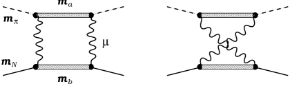
FIG. 4.: The box and crossed-box graphs with masses $m_{a}$ and $m_{b}$ in the intermediate state.

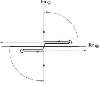
FIG. 5.: Wick rotation and the resulting integration path (bold line) in the complex $q_{0}$ plane. The situation is shown where the two poles 4 and 7 from Eq. (8) have pinched and crossed the imaginary $q_{0}$-axis.

FIG. 6.: The box and various QP approximations for $m_{N}=1,\,m_{\pi}=0.01,\,\sqrt{s}=1.1$ and $t=0$ as a function of the mass $\mu$ of the exchanged particle. In the left and right panels are shown the results corresponding to the graphs (3a) and (3b) respectively. Also are shown the results when the crossed-box is added to the box contribution.

FIG. 7.: The QFT and CET results for the same set of parameters as in Fig. 6 for the case of the graph (3b).

FIG. 8.: The same as Fig. 6, but for $m_{N}=\mu=1,\,m_{\pi}=0.15$ and $t=0$, as a function of the energy $W=\sqrt{s}$.

FIG. 9.: The same as Fig. 6, but for $m_{N}=1,\,m_{\pi}=0.15$ and $t=0$, as a function of the energy $W$. Note that the mass of the exchanged particle for the $t$- and $u$-exchange cases is not the same.

FIG. 10.: The QFT and CET predictions for $m_{N}=1,\,m_{\pi}=0.15$ and $t=0$. Exchange particle masses $\mu=1$ and $\mu=1.31$ have been used for the left and right panels respectively.

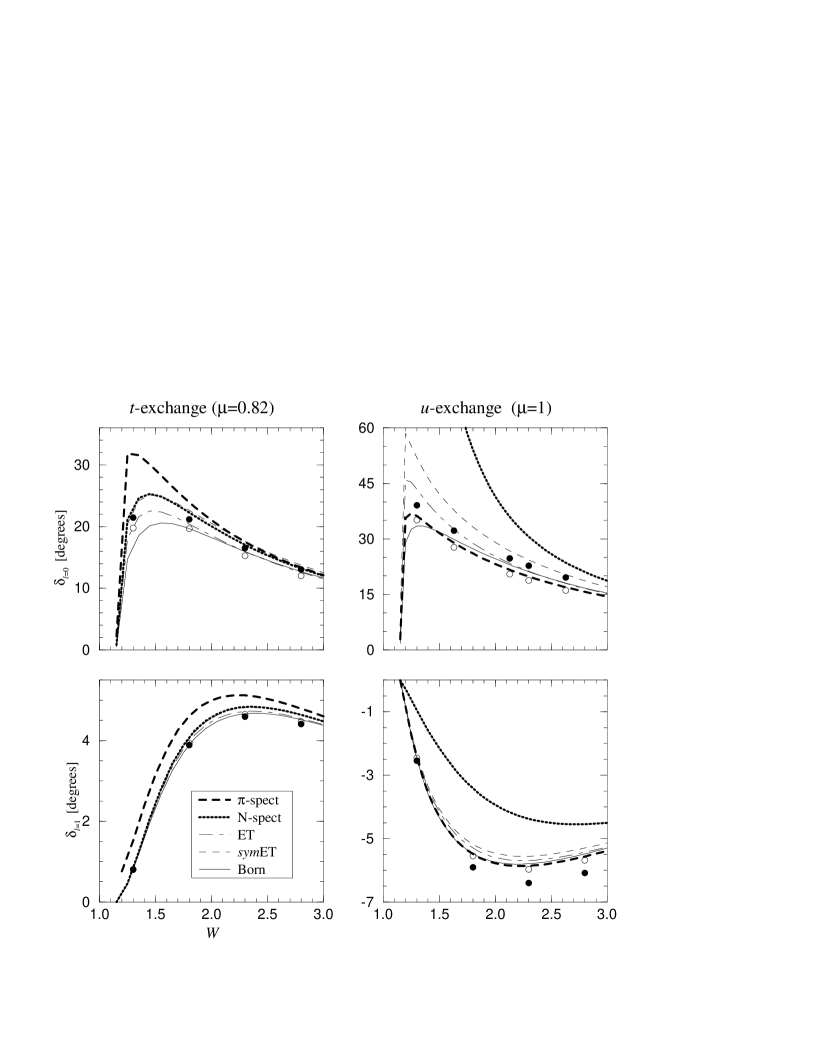
FIG. 11.: S- and P-wave phase shift predictions of various QP approximations with $m_{N}=1$, $m_{\pi}=0.15$, and $g^{2}/(4\pi)=2.0$. In the $u$-exchange S-wave case the nucleon spectator model predicts a phase shift which varies from $\pi$ to zero degrees, i.e. supporting one bound state in this channel. The open dots represent the results of the field-theoretic box graph, the filled dots include the crossed-box graph in addition.

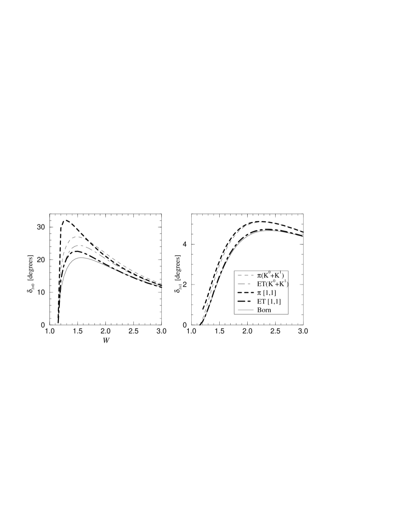
FIG. 12.: Comparison of the phase shifts obtain from perturbation series and the Padé [1,1] approximant for $t$-exchange potential. The same set of parameters as in Fig. 11 are used. In the right panel the predictions of ET(K⁰+K¹) coincide with the ET $[1,1]$ Padé approximant.

REFERENCES

- [1] E. Salpeter, Phys. Rev. 87, 328 (1952).
- [2] A. A. Logunov and A. N. Tavkhelidze, Nuovo Cim. 29, 380 (1963).
- [3] R. Blankenbecler and R. Sugar, Phys. Rev. 142, 1051 (1966).
- [4] V. G. Kadyshevsky, Nucl. Phys. B6, 125 (1968).
- [5] F. Gross, Phys. Rev. 186, 1448 (1969).
- [6] I. T. Todorov, “Quasipotential Approach to the Two-Body Problem in Quantum Field Theory”, in: Properties of the Fundamental Interactions, Vol. 9, part C, ed. A. Zichichi (Compositori, Bologna, 1973) p. 953.
- [7] E. D. Cooper and B. K. Jennings, Nucl. Phys. A500, 553 (1989).
- [8] V. B. Mandelzweig and S. J. Wallace, Phys. Lett. B197, 469 (1987); S. J. Wallace and V. B. Mandelzweig, Nucl. Phys. A503, 673 (1989).
- [9] J. A. Tjon, “Relevance of Relativity in Nuclei”, in: Hadronic Physics with multi-GeV Electrons, Les Houches Series (New Science Publishers, New York, 1990) p. 89.
- [10] J. Fleischer and J. A. Tjon, Phys. Rev. D 21, 87 (1980).
- [11] G. Ramalho, A. Arriaga and M. T. Peña, preprint, nucl-th/9808060.
- [12] F. Gross, Relativistic Quantum Mechanics and Field Theory, (John Wiley & Sons, New York, 1993), Chapter 12.
- [13] F. Gross and Y. Surya, Phys. Rev. C 47, 703 (1993).
- [14] Yu. A. Simonov and J. A. Tjon, Ann. Phys. (NY) 228, 1 (1993).
- [15] M. J. Levine, J. Wright and J. A. Tjon, Phys. Rev. 154, 1443 (1967).
- [16] G. Passarino and M. Veltman, Nucl. Phys. B160, 151 (1979).
- [17] V. Pascalutsa and J. A. Tjon (in preparation); V. Pascalutsa, Ph.D. thesis, University of Utrecht, 1998.
- [18] M. J. Zuilhof and J. A. Tjon, Phys. Rev. C 26, 1277 (1982).
- [19] See, e.g., J. L. Gammel and F. A. McDonald, Phys. Rev. 142, 2245 (1966); H. M. Nieland and J. A. Tjon, Phys. Lett. 27B, 309 (1968).