Physical Review C LBNL-43549

Dynamical simulation of DCC formation in Bjorken rods^∗
Troels C. Petersen and Jørgen Randrup

Nuclear Science Division, Lawrence Berkeley National Laboratory

University of California, Berkeley, California 94720

July 9, 1999

Abstract:

Using a semi-classical treatment of the linear $\sigma$ model, we simulate the dynamical evolution of an initially hot cylindrical rod endowed with a longitudinal Bjorken scaling expansion (a “Bjorken rod”). The field equation is propagated until full decoupling has occurred and the asymptotic many-body state of free pions is then obtained by a suitable Fourier decomposition of the field and a subsequent stochastic determination of the number of quanta in each elementary mode. The resulting transverse pion spectrum exhibits visible enhancements below 200 MeV due to the parametric amplification caused by the oscillatory relaxation of the chiral order parameter. Ensembles of such final states are subjected to various event-by-event analyses. The factorial moments of the multiplicity distribution suggest that the soft pions are non-statistical. Furthermore, their emission patterns exhibit azimuthal correlations that have a bearing on the domain size in the source. Finally, the distribution of the neutral pion fraction shows a significant broadening for the soft pions which grows steadily as the number of azimuthal segments is increased. All of these features are indicative of disoriented chiral condensates and it may be interesting to apply similar analyses to actual data from high-energy nuclear collision experiments.

PACS numbers: 02.60.Cb, 12.39.Fe, 25.75.-q, 29.85.+c

^∗This work was supported by the Director, Office of Energy Research, Office of High Energy and Nuclear Physics, Nuclear Physics Division of the U.S. Department of Energy under Contract No. DE-AC03-76SF00098. TCP was supported in part by the Danish Ministry of Education, the Danish Ministry of Research, Højg $\circ$ard Fonden, and Lørups Mindelegat.

I Introduction

The possibility of forming disoriented chiral condensates (DCC) in high-energy nuclear collisions has gained significant attention in recent years as a means for testing our understanding of chiral symmetry restoration [1, 2, 3]. A crossover from the normal phase, in which chiral symmetry is broken, to a phase with approximately restored chiral symmetry is expected to occur at temperatures of a few hundred MeV. Such energy densities are readily reached during the early stage of an ultrarelativistic nuclear collision and one may therefore expect that approximate restoration of chiral symmetry occurs transiently in the hot collision zone. The subsequent relaxation towards the normal vacuum has a non-equilibrium character due to the very rapid expansion of the system. As a result, the pion field acquires large-amplitude long-wavelength oscillations which may have observable consequences. The suggested signals include an excess of isospin-aligned soft pions with an associated anomalously broad distribution of the neutral pion fraction [4, 5, 6, 7, 8, 9] and, in the electromagnetic sector, a significant excess of photons [10] and dileptons [11, 12].

A few experimental DCC searches have already been carried out [13, 14] but no signals were discerned so far. On the theoretical side, a considerable number of explorative studies of this hypothetical phenomenon have been made over the past several years. However, due to the complicated nature of the problem, most studies have treated fairly idealized scenarios. Therfore the practical observability of the phenomenon is not yet clarified. The purpose of the present work is to treat a somewhat more refined scenario and thus obtain a better basis for making an assessment of the prospects for observing DCC signals and, in the process, provide some guidance for the analysis of the experimental data.

The most popular tool for DCC studies has been the SU(2) linear $\sigma$ model which describes the $O(4)$ chiral field ${\mbox{\boldmath$\phi$}}=(\sigma,\mbox{\boldmath$\pi$})$ by means of a simple effective quartic interaction. This framework has provided instructive insight into the features of the non-equilibrium DCC dynamics [15, 16, 17, 18, 19, 20, 21, 22, 23, 24, 25, 26, 27, 28, 29, 30, 31, 32, 33]. The present study is based on a semi-classical treatment of the standard SU(2) linear $\sigma$ model [25]. The dynamical variable is thus the $O(4)$ chiral field ${\mbox{\boldmath$\phi$}}({\mbox{\boldmath$r$}})=(\sigma,\mbox{\boldmath$\pi$})$ which is subject to a self-interaction of the form $V=\mbox{${\lambda\over 4}$}[\phi^{2}-v^{2}]^{2}-H\sigma$ and, consequently, it is governed by a second-order non-linear equation of motion,

$$[\Box\ +\ \lambda(\phi^{2}-v^{2})]{{\mbox{\boldmath$\phi$}}}\ =\ H\mbox{\boldmath$e$}_{\sigma}\ ,$$ (1)

where $\mbox{\boldmath$e$}_{\sigma}$ denotes a unit vector in the $\sigma$ direction. (Here and throughout we often omit factors of $\hbar$ and $c$ in order not to clutter the formulas.)

In the present study, we wish to consider idealized scenarios that exhibits some of the most important features expected in real collision events, namely rapid longitudinal expansion and finite transverse extension. Generally, the numerical propagation of fields exhibiting significant flow patterns, such as rapid expansion, is practically difficult due to the phase oscillations caused by the local boost. However, for idealized scaling expansions this complication can be eliminated by suitable variable transformations. For the longitudinal scaling expansion considered here [34], it is convenient to replace the usual fixed-frame space-time variables $(x,y,z,t)$ with the comoving variables $(x,y,\eta,\tau)$,

$$t=\tau\cosh\eta\ ,\ z=\tau\sinh\eta\ .$$ (2)

Thus, $\tau=(t^{2}-z^{2})^{1/2}$ is the proper time experienced in a system boosted along the $z$ axis with the local rapidity $\sf y$ equal to the value of $\eta=\mbox{${1\over 2}$}\ln({t+z\over t-z})$. The corresponding form of the field equation of motion is then obtained from the transformation of the d’Alembert operator,

$$\Box\ \equiv\ \partial_{t}^{2}-\partial_{x}^{2}-\partial_{y}^{2}-\partial_{z}^{2}\ =\ {1\over\tau}\partial_{\tau}\tau\partial_{\tau}-\partial_{x}^{2}-\partial_{y}^{2}-{1\over\tau^{2}}{\partial_{\eta}^{2}}\ .$$ (3)

The equation of motion can be readily solved numerically by application of the leapfrog method, once the initial field ${\mbox{\boldmath$\phi$}}({\mbox{\boldmath$r$}})$ and its time derivative ${\mbox{\boldmath$\psi$}}({\mbox{\boldmath$r$}})$ are specified. (To help avoid confusion between the transverse coordinate $y$ and the rapidity $\sf y$, we shall preferentially denote the position in the transverse plane by ${\mbox{\boldmath{{$\rho$}}}}=(x,y)$ in the following, in analogy with the use of ${\bf{k}}=(k_{x},k_{y})$ for the transverse wave number.)

II Bjorken matter

We wish to first consider a macroscopically uniform system, corresponding to infinite matter undergoing a longitudinal Bjorken scaling expansion. Without the scaling expansion, such a system would model infinite uniform matter. We refer to the present expanding generalization as Bjorken matter to capture the essential character of the system by a simple term. Just as ordinary matter approximates conditions prevailing in the bulk region of a finite system, such as a large atomic nucleus, Bjorken matter approximates the conditions in the interior of the rapidly stretching firestreak generated in a central high-energy collision of two large nuclei.

For the numerical calculations, we represent the field on a cartesian lattice in space and impose periodic boundary conditions in all three directions. The initial field configuration is prepared by means of the sampling method developed in Ref. [25]. Thus an initial temperature $T_{0}$ is specified and a field ${\mbox{\boldmath$\phi$}}^{\prime}({\mbox{\boldmath$r$}})$ and its time derivative ${\mbox{\boldmath$\psi$}}^{\prime}({\mbox{\boldmath$r$}})$ are sampled from the corresponding thermal ensemble. This field configuration represents a non-expanding system in thermal equilibrium. In order to obtain an initial field configuration suitable for the expansion scenario, the coordinate $z$ is subsequently identified with the longitudinal variable $\eta$,

$${\mbox{\boldmath$\phi$}}({\mbox{\boldmath{{$\rho$}}}},\eta,\tau_{0})\ \equiv \ {\mbox{\boldmath$\phi$}}^{\prime}({\mbox{\boldmath{{$\rho$}}}},z=\eta)\ ,$$ (4)

$${\mbox{\boldmath$\psi$}}({\mbox{\boldmath{{$\rho$}}}},\eta,\tau_{0})\ \equiv \ {\mbox{\boldmath$\psi$}}^{\prime}({\mbox{\boldmath{{$\rho$}}}},z=\eta)\ ,$$ (5)

where we use $\tau_{0}=1~{}{\rm fm}/c$ for the initial value of the proper time, in accordance with common practice. In this manner it is assured that the local environment at $({\mbox{\boldmath{{$\rho$}}}},\eta)$, when analyzed in a frame boosted with a rapidity $\sf y$ equal to $\eta$, approximates that of matter in equilibrium at the specified temperature $T_{0}$.

A Dynamical evolution

It is instructive to note the evolution of some of the key quantities. Most important is the time dependence of the average field strength, $\underline{{\mbox{\boldmath$\phi$}}}\equiv\langle{\mbox{\boldmath$\phi$}}\rangle$, and the associated dispersion of the field fluctuations around that average, $\delta\phi\equiv[\langle\phi^{2}\rangle-\phi_{0}^{2}]^{1/2}$, where $\phi_{0}\equiv|\underline{{\mbox{\boldmath$\phi$}}}|$. The former represents the O(4) chiral order parameter, while the latter reflects the presence of quasiparticle excitations relative to that constant background field. The dynamical evolution of these quantities is displayed in Fig. 1 for a range of initial temperatures. Initially, at $\tau=\tau_{0}$, the system is hot and the order parameter is significantly reduced relative to its vacuum value of $f_{\pi}=92~{}{\rm MeV}$, with the field fluctuations being substantial (and the more so the higher the value of $T_{0}$). The longitudinal expansion effectively cools the system, causing the field fluctuations to subside (the field dispersion $\delta\phi$ evolves approximately as $1/\sqrt{\tau}$ at large times). This in turn makes the effective potential gradually revert to its vacuum form and the order parameter exhibits a corresponding relaxation. The specific oscillatory evolution is a result of the delicate balance between the expansion rate and oscillation frequency of the evolving effective potential. In the intermediate temperature range where the phase cross over occurs the order parameter exhibits a significant overshoot. These oscillations in the order parameter are reflected in the effective mass tensor for the quasiparticle excitations [29] and, accordingly, the field fluctuations (which depend inversely on the effective mass) exhibit corresponding undulations superimposed on the overall steady decrease in time.

It is helpful to present the combined information in Fig. 1 as a projection onto the chiral phase diagram, in which the order parameter is the abscissa and the field fluctuation is the ordinate. The former characterizes the medium-modified vacuum and the latter is a measure of the degree of excitation relative to that vacuum. The result is displayed in Fig. 2. This figure includes the curve connecting the equilibrium points, starting from ${{\mbox{\boldmath$\phi$}}}_{\rm gs}=(f_{\pi},\mbox{\boldmath$0$})$ at $T=0$ and approaching the vertical axis at large temperatures as chiral symmetry is gradually approached. This curve represents the adiabatic path along which the system would evolve if the expansion were sufficiently slow. We note that the scaling expansion quickly brings the system away from equilibrium, as the cooling of the field fluctuations is immediate while the order parameter requires some time to adjust to the changed effective potential. This inertia leaves the order parameter on the inside of the minimum in the effective potential and it therefore overshoots towards the outside once it gets moving. This pattern is repeated subsequently but on a smaller scale. As a result, the evolution is fairly soon confined to within a narrow neighborhood around the adiabatic path. Nevertheless, the oscillations in the order parameter persist for a long time with a slowly decreasing amplitude. Included on the display is also the critical boundary within which the field is supercritical and spontaneous pair creation occurs [25]. We note that the dynamical paths stay safely away from this boundary, regardless of the value of $T_{0}$, so that no signals of supercriticality should be expected for purely longitudinal expansions, as has already been noted in earlier studies [21, 28].

In order to get an idea of what outcome might be expected, it is helpful to consider the time evolution of the effective pion mass,

$$\mu_{\pi}^{2}(t)\ =\ \lambda[\phi_{0}^{2}+\delta\phi^{2}+2\delta\pi^{2}-v^{2}]\ ,$$ (6)

where $\delta\phi^{2}=\delta\sigma^{2}+\delta\pi_{1}^{2}+\delta\pi_{2}^{2}+\delta\pi_{3}^{2}$ is the total field fluctuation and $\delta\pi^{2}$ denotes the contribution from the field component in the particular isospin direction of the pion considered. This quantity is easily extracted as a by-product of the dynamical calculation and it is displayed in Fig. 3. Since the phase trajectory stays away from the critical region (see Fig. 2), $\mu_{\pi}^{2}$ remains positive throughout. Its evolution can be characterized as an overall steady decrease (approximately inversely proportional to $\tau$) superimposed by a fairly regular oscillation.

It is often instructive to discuss the physics within the framework of the mean-field approximation, which describes the system as a gas of independent quasi-particles endowed with the time-dependent effective mass obtained self-consistently as indicated above (6). In particular, one may consider the evolution of a single pion mode ${\bf{k}}$ being subjected to the calculated effective mass $\mu_{\pi}(t)$. This problem was studied recently in Ref. [35] and it was found that the result can be conveniently expressed by means of the number enhancement coefficient $X_{N}$. This quantity expresses by how much the occupancy of the given mode is enhanced as a consequence of the prescribed time dependence of its mass. Figure 4 shows the resulting enhancement coefficient as a function of the pion momentum, obtained for the four cases depicted in Fig. 3.

On the basis of this schematic analysis, one would expect a significant enhancement for the soft pion modes. It appears that the effect is largest for the intermediate values of $T_{0}$, as might have already been expected from the behavior seen in Fig. 2. Moreover, a careful inspection of the results reveals that $X_{N}(p)$ has two components: a steady decrease resulting from the overall decay of $\mu_{\pi}(t)$ and a bump caused by the parametric amplification of modes matching the frequency of the oscillatory part of $\mu_{\pi}(t)$, with the former being by far the dominant component. (The location at the bump at $200-250~{}{\rm MeV}/c$ corresponds to a pion energy of about half the $\sigma$ mass, as should be expected for the parametric resonance effect [10, 12, 35].)

B Analysis of the final state

As noted above, the continual longitudinal expansion causes the local field fluctuations to subside steadily in the course of time. For the idealized one-dimensional expansion characteristic of Bjorken matter, $\delta\phi^{2}$ decreases as $1/\tau$ for large times (and faster than that when a system with a finite transverse cross section is considered, as in the next section, due to the additional dilution caused by the transverse expansion). Therefore, after a sufficiently long time the system will have decoupled into independently evolving modes of ever decreasing field amplitude. In this asymptotic regime, it is possible to extract well defined values of the observables by suitable analysis of the field configuration. It is useful to note that for large times the longitudinal velocity of a given part of the system is given by $v_{z}\to z/t=\tanh(\eta)$. Thus, in that limit, the coordinate $\eta$ equals the rapidity ${\sf y}=\tanh^{-1}(v_{z})$.

When analyzing the asymptotic field in the Bjorken expansion scenario, it is natural to perform a Fourier transformation in the transverse plane,

$${\mbox{\boldmath$\phi$}}_{\bf{k}}(\eta) = \int{d^{2}{\mbox{\boldmath{{$\rho$}}}}\over\Omega_{\perp}}\ {\mbox{\boldmath$\phi$}}({\mbox{\boldmath{{$\rho$}}}},\eta)\ {\rm e}^{-i{\bf{k}}\cdot{\mbox{\boldmath{{$\rho$}}}}}\ ,$$ (7)

$${\mbox{\boldmath$\psi$}}_{\bf{k}}(\eta) = \int{d^{2}{\mbox{\boldmath{{$\rho$}}}}\over\Omega_{\perp}}\ {\mbox{\boldmath$\psi$}}({\mbox{\boldmath{{$\rho$}}}},\eta)\ {\rm e}^{-i{\bf{k}}\cdot{\mbox{\boldmath{{$\rho$}}}}}\ ,$$ (8)

where ${\bf{k}}=({k}_{x},{k}_{y})$ denotes the transverse wave vector and $\Omega_{\perp}=L_{x}L_{y}$ denotes the transverse area of the spatial lattice. In the present study, we are only interested in observables based on the three pion components of the chiral field. Moreover, while the dynamical treatment of these components is carried out in a cartesian representation, $\mbox{\boldmath$\pi$}=(\pi_{1},\pi_{2},\pi_{3})$, the observations are made in the spherical representation, $\mbox{\boldmath$\pi$}=(\pi_{-},\pi_{0},\pi_{+})$, where the individual components represent the charge states of the pion,

$$\pi_{\pm}\ =\ {1\over\sqrt{2}}[\pi_{1}\pm i\pi_{2}]\ ,\hskip 20.00003pt\pi_{0}\ =\ \pi_{3}\ .$$ (9)

The present treatment yields the time evolution of the classical pion field, $\mbox{\boldmath$\pi$}(x,y,\eta,\tau)$, as described above. In order to make contact with the physical observation, it is necessary to transcribe the emerging field into a quantal many-body state. For this purpose, we associate the asymptotic free field with a coherent state given by

$$|\mbox{\boldmath$\chi$}\rangle = \exp\left\{\sum_{\bf{k}}\int d\eta\left[\mbox{\boldmath$\chi$}_{\bf{k}}(\eta)\cdot\mbox{\boldmath$a$}_{\bf{k}}^{\dagger}(\eta)-\mbox{\boldmath$\chi$}_{\bf{k}}^{*}(\eta)\cdot\mbox{\boldmath$a$}_{\bf{k}}(\eta)\right]\right\}|0\rangle$$ (10)

$$= \exp\left\{\int d^{2}{\mbox{\boldmath{{$\rho$}}}}\int d\eta\left[\mbox{\boldmath$\chi$}({\mbox{\boldmath{{$\rho$}}}},\eta)\cdot\mbox{\boldmath$a$}^{\dagger}({\mbox{\boldmath{{$\rho$}}}},\eta)-\mbox{\boldmath$\chi$}^{*}({\mbox{\boldmath{{$\rho$}}}},\eta)\cdot\mbox{\boldmath$a$}({\mbox{\boldmath{{$\rho$}}}},\eta)\right]\right\}|0\rangle\ .$$ (11)

Here $a^{(j)}({\mbox{\boldmath{{$\rho$}}}},\eta)$ annihilates a pion of type $j$ located at $({\mbox{\boldmath{{$\rho$}}}},\eta)$. It satisfies the usual commutation relation,

$$[a^{(j^{\prime})}({\mbox{\boldmath{{$\rho$}}}}^{\prime},\eta^{\prime}),a^{(j)}({\mbox{\boldmath{{$\rho$}}}},\eta)^{\dagger}]\ =\ \delta_{j^{\prime}j}\ \delta^{(2)}({\mbox{\boldmath{{$\rho$}}}}^{\prime}-{\mbox{\boldmath{{$\rho$}}}})\ \delta(\eta^{\prime}-\eta)\ .$$ (12)

Correspondingly, $a_{\bf{k}}^{(j)}(\eta)$ annihilates a pion of type $j$ located longitudinally at $\eta$ and having the transverse wave vector ${\bf{k}}$, with $[a_{{\bf{k}}^{\prime}}^{(j^{\prime})}(\eta^{\prime}),a_{\bf{k}}^{(j)}(\eta)^{\dagger}]=\delta_{j^{\prime}j}\delta_{{\bf{k}}^{\prime}{\bf{k}}}\delta(\eta^{\prime}-\eta)$.

The coefficients in the expression (10) for the coherent state are given simply in terms of the Fourier expansion coefficients in Eqs. (7-8),

$${\mbox{\boldmath$\chi$}}_{\bf{k}}(\eta)\ =\ \sqrt{\Omega_{\perp}}\left[\sqrt{m_{k}\over 2}{\mbox{\boldmath$\phi$}}_{\bf{k}}(\eta)+{i\over\sqrt{2m_{k}}}{\mbox{\boldmath$\psi$}}_{\bf{k}}(\eta)\right]\ ,$$ (13)

where the transverse mass $m_{k}$ is given by $m_{k}^{2}=m_{\pi}^{2}+k_{x}^{2}+k_{y}^{2}$. The corresponding Fourier expansion yields the complex isovector field appearing in the representation (11) of the coherent state,

$$\mbox{\boldmath$\chi$}({\mbox{\boldmath{{$\rho$}}}},\eta)\ \equiv\ {1\over\sqrt{\Omega_{\perp}}}\sum_{\bf{k}}\mbox{\boldmath$\chi$}_{\bf{k}}(\eta)\ {\rm e}^{i{\bf{k}}\cdot{\mbox{\boldmath{{$\rho$}}}}}\ .$$ (14)

It presents a convenient encoding of the pion field configuration, i.e. the local field strength $\mbox{\boldmath$\pi$}({\mbox{\boldmath{{$\rho$}}}},\eta)$ and its time derivative. We note that the coefficient ${\mbox{\boldmath$\chi$}}_{\bf{k}}(\eta)$ is represented by the basic annihilation operator $\mbox{\boldmath$a$}_{\bf{k}}(\eta)$, while ${\mbox{\boldmath$\chi$}}({\mbox{\boldmath{{$\rho$}}}},\eta)$ is represented by $\mbox{\boldmath$a$}({\mbox{\boldmath{{$\rho$}}}},\eta)$.

The coherent state $|{\mbox{\boldmath$\chi$}}\rangle$ has a number of convenient properties. Most importantly, it is an eigenstate of the annihilation operator,

$$\mbox{\boldmath$a$}_{\bf{k}}(\eta)|\mbox{\boldmath$\chi$}\rangle = {\mbox{\boldmath$\chi$}}_{\bf{k}}(\eta)|{\mbox{\boldmath$\chi$}}\rangle\ ,$$ (15)

$$\mbox{\boldmath$a$}({\mbox{\boldmath{{$\rho$}}}},\eta)|\mbox{\boldmath$\chi$}\rangle = {\mbox{\boldmath$\chi$}}({\mbox{\boldmath{{$\rho$}}}},\eta)|{\mbox{\boldmath$\chi$}}\rangle\ ,$$ (16)

with the eigenvalues being the corresponding $\chi$ coefficients. The two-point density matrix for the state $|\mbox{\boldmath$\chi$}\rangle$ is then given simply in terms of the complex $\chi$ field,

$$\langle\mbox{\boldmath$\chi$}|\mbox{\boldmath$a$}^{\dagger}({\mbox{\boldmath{{$\rho$}}}},\eta)\mbox{\boldmath$a$}({\mbox{\boldmath{{$\rho$}}}}^{\prime},\eta^{\prime})|\mbox{\boldmath$\chi$}\rangle\ =\ \mbox{\boldmath$\chi$}^{*}({\mbox{\boldmath{{$\rho$}}}},\eta)\ \mbox{\boldmath$\chi$}({\mbox{\boldmath{{$\rho$}}}}^{\prime},\eta^{\prime})\ .$$ (17)

Thus the local density of pions with isospin component $j$ is given by the corresponding diagonal element, $d^{3}N^{(j)}/d^{2}{\mbox{\boldmath{{$\rho$}}}}d\eta=|\chi^{(j)}({\mbox{\boldmath{{$\rho$}}}},\eta)|^{2}$. Furthermore, the mean number of such pions emerging with transverse wave vector ${\bf{k}}$ and a rapidity $\sf y$ in the interval $({\sf y}_{1},{\sf y}_{2})$ is then given by

$${\bar{n}}_{\bf{k}}^{(j)}({\sf y}_{1},{\sf y}_{2})\ =\ \int_{{\sf y}_{1}}^{{\sf y}_{2}}d\eta\ |\chi_{\bf{k}}^{(j)}(\eta)|^{2}\ ,$$ (18)

where we have utilized the asymptotic equivalence of the longitudinal coordinate $\eta$ and the rapidity $\sf y$.

In the numerical treatment, the cartesian lattice has spacings of $0.2~{}{\rm fm}$ in the transverse plane and $\Delta\eta=0.2$ longitudinally. Thus the numerical resolution in the longitudinal direction corresponds to a rapidity slice of width $\Delta{\sf y}=0.2$. In the analysis of the results, we consider rapidity intervals $({\sf y}_{1},{\sf y}_{2})$ that have unit length, corresponding to a physical rapidity resolution of one. The corresponding sources are thus made up of five contiguous rapidity slices and we shall refer to them as lumps.

C Transverse spectra

The transverse spectrum of the emerging pions is conveniently expressed as the invariant differential yield, $Ed^{3}N/d^{3}{\mbox{\boldmath$p$}}=d^{3}N/d^{2}{\bf{k}}d{\sf y}$. Due to the boost invariance of the scenario, the resulting inclusive yield does not depend on the rapidity $\sf y$. Moreover, because of the rotational invariance in isospace, it is the same for all three pion states. Finally, the overall axial symmetry of the geometry guarantees that the resulting inclusive observables have azimuthal invariance. Therefore, the transverse spectra depend only on the transverse kinetic energy, $E_{k}=m_{k}-m_{\pi}$.

In order to have a useful reference for judging the calculated spectra, we introduce the equivalent temperature $T_{\rm BE}$ which is determined by matching the calculated spectrum with a corresponding Bose-Einstein equilibrium form. The energy per nucleon determines the temperature,

$$\epsilon\ \equiv\ {E\over N}\ =\ {\sum_{\bf{k}}m_{k}f_{k}\over\sum_{\bf{k}}f_{k}}\ ,\hskip 20.00003ptf_{k}\ =\ [{\rm e}^{m_{k}/T_{\rm BE}}-1]^{-1}\ ,$$ (19)

and the appropriate normalization is determined subsequently by the actual number of particles $N$. This fit is made by considering only a certain energy interval, namely $200<E_{k}<1000$ MeV. The lower cutoff is made in order to permit the extraction of the enhancement of soft pions that is expected to occur. The exclusion of the high momenta is made for numerical convenience: the high-momentum modes (which have only a very small average occupancy) are not treated with great accuracy in the present study as they are computer-demanding but have a negligible effect on the results of present interest. (It has of course been checked that an upwards extension of the upper cutoff on $E_{k}$, with a corresponding better treatment of the high momentum modes, has no import on the results extracted.)

As an example of the outcome of this procedure, the top panel of Fig. 5 shows the transverse spectrum extracted from an ensemble of simulation events having $T_{0}=240~{}{\rm MeV}$, together with the corresponding Bose-Einstein fit. The fit is seen to be quite good for the region $E_{k}>200~{}{\rm MeV}$ within which it has been determined. However, below that region the dynamical result is significantly larger than the corresponding extrapolation of the fit. In order to better bring out this enhancement of the soft pions, we prefer to divide the calculated spectral profile by the corresponding Bose-Einstein fit, thus getting curves that are approximately unity above 200 MeV. The bottom panel of Fig. 5 shows the resulting relative transverse spectra for a number of initial temperatures $T_{0}$. It is evident that the spectra are to a good approximation of equilibrium form above 200 MeV. (The slight shortfall at the higher end of the interval is due to the numerical cutoff in momentum space and it has no import on our present discussion, as discussed above.) Furthermore, equally evident, there is a significant enhancement of the soft pions over a range of $T_{0}$ values, with the effect being largest in the transition temperature region where it reaches up to a factor of two for the softest pions. (It should be noted that the relatively sudden onset of the enhancement below 200 MeV precludes the possibility of obtaining fits of comparable quality by employing an adjustable chemical potential.)

Such a spectral enhancement would probably be within experimental reach. However, since the above results were obtained for idealized scenarios of Bjorken matter, they may well overestimate the effect. It is therefore important to ascertain to what degree this enhancement will persist as an observable signal after the complications of a finite geometry have been included.

III Bjorken rod

We now turn to the study of a more refined scenario in which the system has a finite extension in the transverse plane. Specifically, preserving the longitudinal scaling expansion, we shall replace the matter scenario by a rod-like geometry for which the local environment changes from that of hot Bjorken matter in the bulk to that of vacuum outside through a smooth surface region with a circular cross section. For convenience, we shall refer to such a system as a Bjorken rod. It is illustrated in Fig. 6.

The Bjorken rod combines two features exhibited by the systems produced in real nuclear collisions: a rapid longitudinal expansion and a finite transverse extension. This latter feature implies the presence of a surface region through which the order parameter changes from its initially small value in the hot interior to its vacuum value outside. Because it is both relatively realistic and reasonably tractable, this model scenario has been widely employed in high-energy heavy-ion studies. In the context of DCC studies, it was employed already early on by Asakawa et al. [21]. In that work, the chiral field was taken to be constant in the longitudinal direction, thus rendering the system effectively two-dimensional (with a corresponding reduction of the pressure in the interior). Furthermore, the present study employs a more refined initialization procedure which endows the system with more realistic features, such as a finite correlation length and a surface region through which the field changes smoothly from the hot interior to the exterior vacuum. Finally, whereas the work reported in Ref. [21] was mainly exploratory and rather limited in scope, the present study involves quantitative analyzes of the final state in order to make contact with specific experimental observables. It should be emphasized that the general conclusions drawn in that exploratory work are not affected by the results of the present study.

A Preparation of the rod

For the rod scenario, we again employ a rectangular lattice in $(x,y,\eta)$ and impose periodic boundary conditions in all three directions. In the transverse $xy$ plane, the size of the box should be sufficient to contain the expanding system at times up to the point when the analysis of the final state is made; when this is ensured, the transverse boundary conditions are immaterial. In the longitudinal $\eta$ direction, the periodicity approximates conditions that would prevail if the cylinder were infinitely long, as in the idealized scenario originally considered by Bjorken [34]. Typically the box sides employed are $L_{x}=L_{y}=44\ {\rm fm}$, which suffices for the systems considered, and $L_{\eta}=8$, corresponding to that many units of rapidity.

In preparing the system, we wish the local conditions to correspond approximately to thermal equilibrium at a temperature that decreases steadily from $T_{0}$ inside the bulk region to zero in the vacuum outside. The local temperature $T$ has a Saxon-Woods profile,

$$T(\rho)\ =\ T_{0}~{}[1+{\rm e}^{(\rho-R_{0})/w}]^{-1}\ ,$$ (20)

where $\rho^{2}=x^{2}+y^{2}$. For the surface width parameter we have used $w=0.8~{}{\rm fm}$ and we show results obtained for ensembles of rods with $R_{0}$ equal to 6 or 10 fm. We expect such values of $R_{0}$ to provide a lower bound on the transverse extensions that may be reached for central collisions of gold nuclei at RHIC energies by the time the system has cooled to the specified value of $T_{0}$. This feature is convenient, since a system with a larger transverse extension would be closer to the Bjorken matter scenario considered above (which is approached in the limit $R_{0}\to\infty$).

In order to prepare the initial field configuration for the rod, we proceed at first in the same manner as for the preparation of the matter scenario addressed above and sample the field configuration $({\mbox{\boldmath$\phi$}}_{\rm box},{\mbox{\boldmath$\psi$}}_{\rm box})$ from a thermal ensemble describing macroscopically uniform matter within the overall box containing the calculational lattice. This field configuration can be uniquely decomposed into its spatial average, the order parameter, and the remainder, the fluctuating part of the field,

$${\mbox{\boldmath$\phi$}}_{\rm box}({\mbox{\boldmath{{$\rho$}}}},\eta)\ = \ \underline{{\mbox{\boldmath$\phi$}}}\ +\ {\mbox{\boldmath$\delta\phi$}}({\mbox{\boldmath{{$\rho$}}}},\eta)\ ,$$ (21)

$${\mbox{\boldmath$\psi$}}_{\rm box}({\mbox{\boldmath{{$\rho$}}}},\eta)\ = \ \underline{{\mbox{\boldmath$\psi$}}}\ +\ {\mbox{\boldmath$\delta\psi$}}({\mbox{\boldmath{{$\rho$}}}},\eta)\ .$$ (22)

In order to obtain the field configuration describing the initial state of the rod, $({\mbox{\boldmath$\phi$}}_{\rm rod},{\mbox{\boldmath$\psi$}}_{\rm rod})$, we rescale the two parts based on the specified local temperature $T(\rho)$ and then recombine them into the desired initial conditions,

$${\mbox{\boldmath$\phi$}}_{\rm rod}({\mbox{\boldmath{{$\rho$}}}},\eta,\tau_{0})\ = \ g(\rho)[\underline{{\mbox{\boldmath$\phi$}}}-{\mbox{\boldmath$\phi$}}_{\rm gs}]\,+{\mbox{\boldmath$\phi$}}_{\rm gs}\ +\ \mbox{\boldmath$h$}(\rho)\circ[{\mbox{\boldmath$\delta\phi$}}({\mbox{\boldmath{{$\rho$}}}},\eta)-\underline{{\mbox{\boldmath$\phi$}}}]\,+\underline{{\mbox{\boldmath$\phi$}}}\ ,$$ (23)

$${\mbox{\boldmath$\psi$}}_{\rm rod}({\mbox{\boldmath{{$\rho$}}}},\eta,\tau_{0})\ = \ g(\rho)[\underline{{\mbox{\boldmath$\psi$}}}-{\mbox{\boldmath$\psi$}}_{\rm gs}]+{\mbox{\boldmath$\psi$}}_{\rm gs}\ +\ \mbox{\boldmath$h$}(\rho)\circ[{\mbox{\boldmath$\delta\psi$}}({\mbox{\boldmath{{$\rho$}}}},\eta)-\underline{{\mbox{\boldmath$\psi$}}}]+\underline{{\mbox{\boldmath$\psi$}}}\ ,$$ (24)

where ${\mbox{\boldmath$\phi$}}_{\rm gs}=(f_{\pi},\mbox{\boldmath$0$})$ and ${\mbox{\boldmath$\psi$}}_{\rm gs}=(0,\mbox{\boldmath$0$})$ are the vacuum values. The scaling coefficient for the order parameter is obtained from the magnitudes of the corresponding order parameters, $g(\rho)=[\phi_{0}(T(\rho))-f_{\pi}]/[\phi_{0}(T_{0})-f_{\pi}]$, where $\phi_{0}(T)$ denotes the magnitude of the order parameter in thermal equilibrium at the specified temperature $T$. The scaling coefficient for the fluctuations depends on the particular chiral component, so $h$ is a diagonal O(4) tensor with the following elements,

$$h_{\sigma}(\rho)\ =\ \left({\delta\sigma^{2}_{T}\over\delta\sigma^{2}_{T_{0}}}\right)^{1\over 2}\ ,\,\,\ h_{\pi}(\rho)\ =\ \left({\delta\pi^{2}_{T}\over\delta\pi^{2}_{T_{0}}}\right)^{1\over 2}\ .$$ (25)

and $\circ$ denotes the corresponding O(4) scalar product. Here $\delta\sigma^{2}_{T}$ denotes the thermal equilibrium value of the fluctuation in the $\sigma$ component of the chiral field and $\delta\pi^{2}_{T}$ is the thermal fluctuation in (any) one of the pion components. These are calculated by the semi-classical mean-field method [25]. (It should perhaps be noted that in principle one needs to take account of the fact that generally the order parameter $\underline{{\mbox{\boldmath$\phi$}}}$ is not fully aligned with the O(4) $\sigma$ direction and hence the $\sigma$ and $\pi$ field fluctuations are not independent. Rather, it is the fluctuations parallel and perpendicular to the order parameter, $\delta\phi_{\parallel}$ and ${\mbox{\boldmath$\delta\phi$}}_{\perp}$, that decouple (i.e. their quasiparticle mass tensor is diagonal). However, for the quite large systems considered here, $\underline{{\mbox{\boldmath$\phi$}}}$ is practically fully aligned in the $\sigma$ direction and so we do not need to be concerned with that distinction in our discussion. Nevertheless, for the sake of generality, the numerical treatment performs the proper O(4) diagonalization and rotation when the field preparation is done [25].)

By proceeding in the manner described above, we ensure that the local environment, as characterized by the order parameter and the field fluctuations, reflects approximately thermal equilibrium in matter held at the local temperature $T$, which decreases from its bulk value $T_{0}$ to zero according to the prescribed radial profile (20).

The initial system is illustrated in Fig. 7 for $T_{0}=240~{}{\rm MeV}$. It shows the radial dependence of a number of key quantities: the local temperature $T$, the order parameter $\phi_{0}$, the field fluctuations $\delta\sigma$ and $\delta\pi$, and the effective masses $\mu_{\sigma}$ and $\mu_{\pi}$. Since the local temperature drops steadily as a function of the transverse distance $\rho$, moving out along the abscissa corresponds to reducing the temperature (though not at a steady rate). As one moves out through the surface, the order parameter increases steadily from its reduced value ($\approx 27~{}{\rm MeV}$) in the hot bulk region towards its vacuum value $f_{\pi}$ ($=92~{}{\rm MeV}$), and the local thermal fluctuations drop correspondingly towards zero. (Since generally $\mu_{\sigma}>\mu_{\pi}$, the fluctuations along a pion direction exceed those in the $\sigma$ direction.) The resulting profiles of the effective masses also reflect their temperature dependences: Starting from nearly degenerate values ($\approx 300~{}{\rm MeV}$) in the hot interior, where chiral symmetry is approximately restored, $\mu_{\pi}$ and $\mu_{\sigma}$ diverge steadily towards their free values of $138~{}{\rm MeV}$ and $600~{}{\rm MeV}$, respectively. For higher values of the central temperature $T_{0}$, the central value of the order parameter is smaller and the effective masses are larger (and even closer in value) and $\mu_{\sigma}$ will in fact exhibit a dip in the surface region as the local temperature passes through the critical region [25, 36].

B Rod dynamics

After the preparation of the field configuration of the rod, the dynamical propagation is readily obtained by solving the field equation (1) as was done for the matter configurations. Since the system is no longer macroscopically uniform, it is more complicated to discuss, but it is especially instructive to see how the bulk region develops. For this purpose, we probe a circular region in the interior of the rod and extract the corresponding values of the order parameter and field fluctuations. The resulting evolution of the order parameter and the field fluctuations is illustrated in Fig. 8 for a rod with $T_{0}=240~{}{\rm MeV}$ and $R_{0}=6~{}{\rm fm}$. The corresponding quantities for Bjorken matter prepared with the same value of $T_{0}$ are also shown. It is seen that the environment in the interior of the rod evolves in a manner quantitatively very similar to that of the corresponding matter scenario throughout the first complete oscillation of the the order parameter, which takes about $4~{}{\rm fm}/c$. At around that point in time, the decompression wave has arrived from the rod surface and the self-generated transverse expansion now extends over the entire cross section of the rod. As a consequence, the relaxation progresses faster than it would in matter where this effect is absent.

This feature is also brought by the the corresponding dynamical paths on the phase diagram, as shown in Fig. 9. The initial location of the point for the rod interior differs slightly from that of the equilibrium matter because of the finite size of the hollow cylindrical volume sampled. But apart from this minor difference, the rod path tracks the matter path closely for the first several time units, as brought out by the proximity of the corresponding time markers at $\tau=1,2,3,4,5~{}{\rm fm}/c$. Beyond that time, the paths begin to diverge, as shown by the subsequent time markers at $\tau=10,20,30~{}{\rm fm}/c$. From around $20~{}{\rm fm}/c$, or so, the rod interior is quite close to the vacuum point, whereas the environment in the matter scenario remains significantly excited for a much longer time.

The quicker relaxation of the field for the rod configuration is also reflected in the behavior of the effective pion mass. This is illustrated in Fig. 10 for the same case. Again we see that through the first several time units the effective mass in the interior of the rod follows closely the evolution of the effective mass extracted for the corresponding matter scenario, but it then drops much faster towards the free value. Furthermore, the oscillations in the effective mass persist for quite a long time, thus making it possible to achieve a significant degree of parametric amplification.

C Transverse spectra

We now consider a number of specific observables that are practically accessible in the analysis of actual experimental data. First we consider the transverse spectra of the emerging pions, $Ed^{3}N/d^{3}{\mbox{\boldmath$p$}}=d^{3}N/d^{2}{\bf{k}}d{\sf y}$. As was the case for the Bjorken matter scenarios, the transverse spectral shape is well approximated by an equilibrium form above kinetic energies of $200~{}{\rm MeV}$ or so. We therefore proceed in the same manner and extract a corresponding equivalent temperature, $T_{\rm BE}$, for each case considered.

The values obtained for $T_{\rm BE}$ are shown in Table I for a range of initial bulk temperatures $T_{0}$ and a rod radius of $R_{0}=6~{}{\rm fm}$ (the values of $T_{\rm BE}$ are rather insensitive to $R_{0}$). We note that they increase steadily with $T_{0}$, as one would expect. It might at first seem surprising that $T_{\rm BE}$, the effective temperature characterizing the transverse spectrum of the final pions, can exceed $T_{0}$, the specified bulk temperature of the initial state. However, it should be kept in mind that the quasipions in the bulk of the initial system have an effective mass $\mu_{\pi}$ that exceeds the free value $m_{\pi}$ by hundreds of MeV, due to the self-interaction of the thermally agitated field. As the system expands and cools, the interaction energy energy is converted primarily into kinetic energy and hence the spectrum hardens.

The resulting ratio between the dynamical spectrum and the corresponding Bose-Einstein form is displayed in Fig. 11 for $T_{0}=240~{}{\rm MeV}$, together with the corresponding matter result. While the quality of the fit for rods is as good as for matter, the ensuing soft enhancements are generally smaller. This is not surprising, since the bulk conditions prevail in only part of the rod configuration and, moreover, the transverse expansion tends to suppress the oscillatory relaxation causing the enhancement.

Figure 12 shows the relative excess of soft pions as a function of the initial bulk temperature $T_{0}$ for Bjorken rods with $R_{0}$ equal to 6 and 10 fm. We see that the effect begins to manifest itself at temperatures above 200 MeV, for which the bulk value of the order parameter is significantly reduced from its vacuum value, and it exhibits a broad maximum at roughly $T_{0}=240-280~{}{\rm MeV}$ before gradually subsiding at higher $T_{0}$. The larger the rod radius $R_{0}$, the larger the enhancement, as one would expect, since the system is then better approximated by bulk matter. The excess of pions below 200 MeV is of the order of ten per cent. Though significantly smaller than that obtained for infinite matter, such enhancements are nevertheless still significant and should be well within observable reach.

Since the excess pions reflected in the spectral enhancement are produced by the coherent oscillation of the order parameter, their properties are expected to differ from the regular pions. Therefore, in order to better bring this out, it is useful to consider the soft and hard pions separately in the following analyses.

D Multiplicity distributions

We now turn to the discussion of the resulting multiplicity distributions. By invoking the relation (18), it is straightforward to calculate the expected number of pions in a given rapidity interval and within a specified transverse energy bin. Of course, this result varies from event to event, since the field configurations vary at the microscopic level as a result of the thermal fluctuations in the ensemble of initial states.

For a given value of the expected number $\bar{n}$, the actual number of particles emerging is a stochastic variable $n$, since the state described by a given field has no well-defined particle number. Generally, knowledge of the classical field alone does not allow a construction of the underlying quantum many-particle state. However, in the present case where we have made the common assumption that the final quantum state is of standard coherent form (see Eq. (10)), it is elementary to show that the associated multiplicity distribution is of Poisson form. Thus, the probability for obtaining a specified number of particles with transverse momentum ${\bf{k}}$ within a given rapidity interval, $n_{\bf{k}}^{(j)}({\sf y}_{1},{\sf y}_{2})=n$, is given by

$$P_{\bar{n}}(n)\ =\ {\bar{n}^{n}\over n!}\ {\rm e}^{-\bar{n}}\ ,$$ (26)

where $\bar{n}=\bar{n}_{\bf{k}}^{(j)}({\sf y}_{1},{\sf y}_{2})$ is the given mean value (18). We can therefore readily pick the actual number of $j$-type pions emerging from each particular rapidity slice with the transverse momentum ${\bf{k}}$. The Poisson distributions form a closed algebra under convolution, with the corresponding mean values being additive, $P_{a}*P_{b}=P_{a+b}$. Consequently, the total number of particles emerging with a given transverse wave vector ${\bf{k}}$ from a given rapidity lump can be obtained equivalently by either sampling the multiplicities for each of the constituent slices from the corresponding individual Poisson distributions, or by sampling the the total multiplicity $n_{\bf{k}}$ from the corresponding combined Poisson distribution. Different values of ${\bf{k}}$ can be combined in a similar manner, for example to obtain the number of pions emerging within a specific energy bin. It is thus clear that the resulting calculated statistical multiplicity distributions do not depend on the specific computational procedure employed for the stochastic sampling.

As an illustration, we show in Fig. 13 both the expected and the actual multiplicity as obtained for a single event. It follows from the above remarks that the fluctuations in the calculated rapidity density has two different sources. One is the variation in the details of the resulting field configuration from event to event and from one rapidity lump to another (giving rise to the smooth curves in Fig. 13). The other is the subsequent Poisson sampling of the actual multiplicity based on the smooth average given by the calculated final field (leading to the fluctuating histogram in the figure).

In order to investigate whether the resulting multiplicity distributions contain deviations from the relatively trivial Poisson statistics, we have extracted the associated factorial moments. Because of the enhancement of the soft pions seen in the transverse spectra, we consider the pions below and above 200 MeV separately. For multi-particle final states, one may define the following factorial moments,

$${\cal M}_{m}\ \equiv\ \prec N(N-1)\cdots(N-m+1)\succ\ .$$ (27)

Here $N$ is the number of pions emitted by a given rapidity lump of unit length and the average is over all lumps in a sample of events prepared in the same manner (i.e. same bulk temperature $T_{0}$ and rod radius $R_{0}$); the contribution vanishes for a lump with a multiplicity smaller than the particular order $m$. For a Poisson multiplicity distribution characterized by the mean multiplicity $\bar{N}$, the factorial moments are simply given by ${\cal M}_{m}=\bar{N}^{m}$. Therfore we prefer to consider the reduced factorial moments, ${\cal M}_{m}/\bar{N}^{m}$, which are then all unity for a Poisson multiplicity distribution. Since $\bar{N}$ is not available experimentally, we use instead the average of the observed multiplicities for each lump, $\prec N\succ$. This should provide a good approximation, since the lumps are all macroscopically equivalent.

Figure 14 shows the relative factorial moments obtained for a sample of Bjorken rods prepared with $T_{0}=250~{}{\rm MeV}$ and $R_{0}=6~{}{\rm fm}$. (We consider from now on systems prepared with $T_{0}=250~{}{\rm MeV}$, since the soft enhancement is largest near this temperature.) While the hard pions appear to be perfectly consistent with pure Poisson statistics, the soft pions exhibit a significant non-poissonian behavior. The character of the deviation of the soft factorial moments suggests that the source occasionally emits anomalously many pions, as one would expect if some modes are especially amplified. This feature is consistent with the enhancement of the soft spectrum and it can also be explored by other means of analyzing the data for anomalous fluctuations.

E Azimuthal emission patterns

When averaged over events, the emission probability has overall cylindrical symmetry, due to the symmetry of the initial ensemble of fields. Similarly, due to the boost invariance of the ensemble, the averaged emission probability is independent of the rapidity. And, thirdly, the isospin invariance of the ensemble guarantees that all three types of pion behave similarly after the event average has been carried out. Though each individual lump retains these symmetries in a macroscopic sense, texture exists at the microscopic level. This important feature is manifested as fluctuations in the underlying mean multiplicities $\bar{n}_{\bf{k}}^{(j)}({\sf y}_{1},{\sf y}_{2})$, from one rapidity interval to the next and from event to event.

The fluctuations in the azimuthal pattern of the asymptotic pion field can be elucidated by means of the following multipole moments,

$$\tilde{\alpha}_{M}^{(j)}({\sf y}_{1},{\sf y}_{2})\ \equiv\ {1\over E_{\perp}}|\sum_{\bf{k}}\bar{n}_{\bf{k}}^{(j)}({\sf y}_{1},{\sf y}_{2})E_{k}\ {\rm e}^{iM\phi_{\bf{k}}}|\ .$$ (28)

The weighting by the transverse kinetic energy $E_{k}\equiv m_{k}-m_{\pi}$ ensures that particles emitted with very low transverse momentum have little effect, as is reasonable since their particular azimuthal direction is physically insignificant. Because of the spectral enhancement of the soft pions discussed above, we extract the multipole strength distribution for soft and hard pions separately. Finally, $E_{\perp}\equiv\sum_{\bf{k}}\bar{n}_{\bf{k}}E_{k}$ denotes the total mean transverse kinetic energy of the soft or hard pions emitted by a given lump. The division by $E_{\perp}$ ensures that $\tilde{\alpha}_{0}$ is always unity. (It should perhaps be added that the rather large transverse dimensions of the spatial lattice ensures that the corresponding resolution in the wave number ${\bf{k}}$ is sufficiently fine to render the extracted multipole moments coefficients numerically reliable for values of the multipolarity $M$ comfortably beyond the point when their values have become insignificant.)

In each individual event, and for each of the three pion types separately, the multipole moments are calculated for the pions arising from each separate rapidity lump. Because of the independence of different events, the isospin symmetry, and the longitudinal boost invariance, respectively, all the individual lumps present equivalent sources and hence we may perform a subsequent average, yielding $\prec\tilde{\alpha}_{M}\succ$.

The resulting ensemble average azimuthal multipole strength function is displayed in Fig. 15 for the soft modes of the asymptotic pion field. Two different Bjorken rod scenarios are displayed, both having the initial bulk temperature is $T_{0}=250~{}{\rm MeV}$, but the initial radius $R_{0}$ being either 6 fm or 10 fm. In order to get an idea of the significance of the extracted values, we have calculated an auxiliary set of moments, $\tilde{\alpha}_{M}^{\rm random}$, obtained by turning each individual emission direction $\phi_{\bf{k}}$ by a random angle before evaluating the multipole moment.

The azimuthal coefficients for soft pions, considered as a function of the multipolarity $M$, start out well above the noise level, then exhibit a gradual drop-off. For high multipolarities, the moments approach zero because the high-frequency components of the field are suppressed by the initial thermal weight.

The behavior of the multipole strength provides some information on the domain structure of the source, as we shall now discuss. First we note that the attenuation of the strength with increasing multipolarity $M$ can be reasonably well approximated by a simple gaussian fit. The fit makes it possible to extract the dispersion of the curve, $\Delta M$. Employing the usual inverse relationship between conjugate variables, we may then obtain the azimuthal correlation length, $\Delta\phi=1/\Delta M$. Thus, if the effective transverse size of the source is $R$, the spatial domain size in the source is given by $\approx$$R\Delta\phi$. For the two scenarios having the initial rod radius $R_{0}$ equal to 6 and 10 fm, we extract $\Delta M$ as 5.03 and 8.84, leading to values of $\Delta\phi$ equal to 11.4${}^{\circ}\hskip 3.99994pt$ and 6.5${}^{\circ}\hskip 3.99994pt$, respectively. Since $R_{0}\Delta\phi$ is thus approximately the same in the two scenarios, the spatial correlation length at the effective emission time appears to be independent of the initial radius of the rod. This is as one would expect if that quantity reflects the conditions in the source at the time of effective decoupling.

The corresponding multipole coefficients extracted for the hard pions are shown in Fig. 16. They are initially an order of magnitude smaller than those for the soft pions but they exhibit a significantly gentler fall-off with the multipolarity $M$, suggesting a correspondingly narrower angular correlation. This is consistent with the general expectation that harder pions exhibit a smaller spatial correlation length. As for the soft modes, the wider rod yields smaller multipole coefficients.

The above discussion has been based on the pion field, rather than the resulting particles. The field is a relatively smoothly varying function of position and it governs the mean number of quanta in the various elementary modes. The actual final state of particles is then determined stochastically, as described in the preceding. This feature tends to add a certain degree of noise to the azimuthal pattern exhibited by the underlying field, as we shall now illustrate. When the analysis is made in terms of the emitted particles, as is necessarily the case in actual experiments, the definition of the multipole moments should be modified appropriately,

$$\alpha_{M}\ \equiv\ {1\over E_{\perp}}|\sum_{n}E_{n}\ {\rm e}^{iM\phi_{n}}|\ ,\\$$ (29)

where $n$ enumerates the $N$ particles emerging in the particular kinematic domain under consideration and $E_{n}\equiv m_{n}-m_{\pi}$ is the transverse kinetic energy of an individual particle emitted in the azimuthal direction $\phi_{n}$. Furthermore, $E_{\perp}\equiv\sum_{n}E_{n}$, is the total transverse energy of the $N$ particles, so that $\alpha_{0}$ is unity.

Figure 17 shows the multipole strength coefficients $\alpha_{M}$ extracted for the case with $R_{0}=6~{}{\rm fm}$. As was the case for the coefficients extracted from the underlying field, the particle-based coefficients acquire significant values for low values of the multipolarity $M$. As the multipolarity is increased, $\alpha_{M}$ approaches the statistical noise level, $\alpha^{\rm random}_{M}$, obtained as above by randomizing the direction of each emitted pion. This is what one would expect since the angular distribution is now a sum of $\delta$-functions and thus contains all the high multipolarities equally. To better bring out the features of the non-statistical behavior, we subtract the average value of the noise, $\langle\alpha^{\rm random}\rangle$, before making the fit (hence some of the resulting values are slightly negative for large $M$).

Once the average noise has been subtracted, the multipole strength distribution based on the emitted particles is quantitatively very similar to the one based on the underlying asymptotic field. This is true for both values of $R_{0}$ shown. It thus appears possible to gain experimental access to the correlation properties of the field itself, even though the particles, on which the observations are necessarily based, are obtained from the field by a stochastic process.

The above analysis suggest that an extraction of azimuthal moments for observed soft pions may yield non-trivial information on the domain structure in the system. In this undertaking, it would probably be useful to explore the effect of adjusting the cuts in both rapidity and transverse energy, so as to tune the extraction procedure to the specific character of the sources produced.

F Neutral pion fraction

The distribution of the neutral pion fraction $f\equiv N_{\pi^{0}}/N_{\rm tot}$ has received considerable attention as a DCC diagnostic because an idealized fully isospin-polarized source would yield an anomalously wide distribution, $P_{0}(f)=1/2\sqrt{f}$, rather than a narrow peak around the average value $f=\mbox{${1\over 3}$}$. Indeed, experiments have been devoted to the search for anomalous behavior of the neutral pion fraction [13, 14]. However, such an undertaking is quite difficult, partly because the signal is expected to be carried by only the soft pions and partly because the extraction of $f$ requires the simultaneous event-by-event measurement of both charged and neutral pions. These practical problems not withstanding, $P(f)$ remains a very instructive quantity in the DCC context and we have therefore extracted it as well.

As above, we consider soft and hard pions separately. In each case, we calculate the neutral pion fraction $f$ for each rapidity lump and construct its distribution $P(f)$ by binning the $f$ values obtained from all lumps and events. Since all extracted distributions $P(f)$ appear well-peaked around their common average of one third, it suffices for our discussion to characterize a given distribution by its variance $\sigma_{f}^{2}=\langle f^{2}\rangle-\langle f\rangle^{2}$. It is elementary to show that the extreme idealized distribution $P_{0}(f)$ has the variance $\sigma_{0}^{2}=4/45$ and that $N$ such sources of equal strength have the variance $\sigma_{f}^{2}=\sigma_{0}^{2}/N$ [29]. More generally, one may consider an assembly of $N$ different sources, with individual distributions $P_{i}(f_{i})$. If the strength (i.e. the total multiplicity) of a given source is $\nu_{i}$, the neutral fraction for the entire assembly is given by $f=\sum_{i}\nu_{i}f_{i}/\sum_{i}\nu_{i}$ and its distribution is therefore given by

$$P(f)\ =\ \left[\prod_{i=1}^{N}\int df_{i}\ P_{i}(f_{i})\right]\ \delta(f-\sum_{i=1}^{N}\nu_{i}f_{i}/\sum_{i=1}^{N}\nu_{i})\ .$$ (30)

It is easy to verify that the mean value of $f$ remains equal to one third. Moreover, a slightly more elaborate calculation yields the expression for the variance of the combined distribution,

$$\sigma_{f}^{2}\ =\ {\sum_{i}\nu_{i}^{2}\over(\sum_{i}\nu_{i})^{2}}\ \sigma_{0}^{2}\ .$$ (31)

If the isospin polarizations of all the elementary modes ${\bf{k}}$ are totally independent, then the above formula (31) applies and it is possible to predict the resulting width $\sigma_{f}$ by substituting the mean multiplicities $\bar{n}_{\bf{k}}=\sum_{j}\bar{n}_{\bf{k}}^{(j)}$ for the strengths $\nu_{i}$. However, in actuality the pion field changes smoothly from one mode to the next and so the isospin directions of neighboring modes are somewhat correlated. Consequently, we expect the actual $\sigma_{f}$ to be significantly larger than the lower bound provided by (31) and indeed this turns out to be the case.

In the present discussion, we calculate the neutral fraction both on the basis of the asymptotic fields, which govern the mean multiplicities for each elementary mode, and on the basis of the resulting particles, which are picked stochastically from those mean multiplicities (see above). Table II lists the resulting widths $\sigma_{f}$ for Bjorken rods with radii $R_{0}$ equal to either 6 or 10 fm. We notice that when the transverse size of the system is increased, the distribution becomes narrower, as expected since more domains can be accommodated across the source. In addition to considering the usual lumps covering one unit of rapidity each, we have also calculated $\sigma_{f}$ by separating each lump into its five constituent slices. Naturally, the associated decrease of the source size causes $P(f)$ to broaden. However, the the fact that the variance grows by less than a factor of five is a reflection of the fact that the effective domain size extends beyond a single slice, so that neighboring slices are not independent with regard to their isospin alignment. Finally, we notice that the distributions based on the particles (which are the observable quantities) are generally significantly broader than those based on the underlying fields.

It is also instructive to study how $P(f)$ evolves when the data is separated into azimuthal sections. Thus, each individual lump is subdivided into $m$ equally large azimuthal sections and $P(f)$ is calculated for each such source. The result is illustrated in Fig. 18 which shows the width of $P(f)$ as a function of the number of angular sections $m$, for both soft and hard pions. Generally $P(f)$ broadens as the width of the angular section is decreased, as one would expect since the effective number of contributing domains goes down. However, $\sigma_{f}$ will not approach the value for a single idealized source, as $m\to\infty$, because the transverse extension of the source exceeds the correlation length and so the source will never become fully aligned in isospace. This feature is similar to what was obtained when idealized rods were sliced ever finer in rapidity [38]. Moreover, as we have seen above, the soft pions lead to a significantly broader distribution than the hard ones.

IV Discussion

In the present work, we have employed the standard linear $\sigma$ model to study systems prepared with a cylindrical geometry and endowed with a longitudinal Bjorken scaling expansion. Such a scenario is an idealized representation of what might be produced in a central ultrarelativistic nuclear collision. After their preparation with an interior temperature in or above the chiral transition region, the system is left free to evolve self-consistently, until the combined longitudinal and transverse expansion has brough it into the simple asymptotic regime of free dispersion where a well-defined analysis can be made. We have studied a number of observables related to the emerging pions, for the purpose of exploring the persistence of signals reflecting the preceding non-equilibrium relaxation of the chiral field.

Most important, and also most easily checked experimentally, is the emergence of a surplus of pions with transverse kinetic energies below $200~{}{\rm MeV}$, relative to the expectation based on a simple extrapolation of the harder part of the spectral profile, which turns out to be quite well approximated by a Bose-Einstein form. The excess of soft pions calculated in this manner depends on the initial bulk temperature of the rod, $T_{0}$, as well as on its radius, $R_{0}$, and it is largest for $T_{0}=240-280~{}{\rm MeV}$. In the optimal range of $T_{0}$, the total relative excess of pions below $200~{}{\rm MeV}$ amounts to about $10\%$ and $15\%$ for $R_{0}$ equal to 6 and 10 fm, respectively. Since the transverse radius of the source is likely to be larger than $10~{}{\rm fm}$ for central collisions at RHIC, the present rod calculations are expected to underestimate the effect. Thus, if indeed the effect is present, it ought to be readily visible in the data.

Since the additional soft pions arise from the oscillatory relaxation of the chiral order parameter in the interior of the source, they are expected to be non-statistical and partially isospin polarized. In order to elucidate the degree to which remnants of these features are identifiable in the final state, we have performed various event-by-event analyses on the calculated results based on samples of several tens of separate rod evolutions.

In one type of analysis, we have extracted the factorial moments of the pion multiplicity distribution associated with a rapidity interval of unit width. We found that while the hard pions display a perfect Poisson multiplicity distribution, the soft pions show a significant non-poissonian behavior, with the reduced factorial moments growing approximately linearly with order. A similar multiplicity analysis should be readily possible with the multi-particle data collected by the STAR TPC, for example.

In another series of analyses, we sought to elucidate the azimuthal structure of the final emission pattern by extracting the corresponding multipole strength function. These analyses were made both for the asymptotic field, which is not directly detectable, and for the resulting particles. The strength was found to decrease steadily with multipolarity in an approximately gaussian manner, thus making it possible to extract an angular correlation length. These studies suggested that the spatial correlation length in the source (the “domain size”) is independent of the initial rod radius, but significantly larger for the soft pions. Moreover, these features were not affected by the stochastic transition from field to particles, thus suggesting that such angular analysis of the actual data may be informative.

Finally, we extracted the distribution of the neutral pion fraction for the event samples considered, since this quantity has played a central role in the discussion of disoriented chiral condensates (though it is practically difficult to measure). Information about the correlation length, and hence the domain structure, was obtained by dividing each rapidity lump into azimuthal segments before calculating the neutral fraction. We found that the fraction distribution widens steadily as the number of segments is increased and, importantly, that the width associated with the soft pions is several times larger than that for the hard pions.

Even though the present study is more refined than earlier treatments, with regard to the dynamical scenario and the analysis of the outcome, it is still highly idealized in a number of respects. Especially important are the following limitations. First, at the most basic level, the linear $\sigma$ model is an effective field theory containing merely a few mesonic fields, rather than the basic quark-gluon degrees of freedom. This simplification may become especially important at the early stage when the high excitation is expected to largely dissolve the hadronic correlations in the interior of the system. Second, even at the effective level, a full non-equilibrium real-time quantum-field treatment is presently far beyond practicality. Instead, we are resorting to a semi-classical treatment. While perhaps quite adequate in many respects [40], this treatment is expected to generally underestimate the enhancement in the pion yield caused by the non-equilibrium dynamics [35]. Third, the commonly employed SU(2) version of the linear $\sigma$ model entirely ignores strangeness. However, this degree of freedom is expected to become significantly agitated once the temperature exceeds the mass of the strange quark, as is the case at the early stage of the evolution. The extension of the model to SU(3) has been found to have significant effects [39]. Fourth, the initial state is obtained by sampling a (suitably modulated) field configuration from a thermal ensemble. The sampling procedure relies on the mean-field approximation and thus the initial state contains only a minimum of many-particle correlations. This feature might become reflected in a corresponding paucity of non-trivial correlations in the final state. An analogous problem concerns the transcription of the final classical field configuration to a specific quantum state. Since our prescription assigns a standard coherent state, it is likely to provide an oversimplification of the many-body correlations present. (Indeed, recent studies suggest that the parametric amplification mechanism behind the spectral enhancement in fact destroys the simple coherent form of the state [35].) Fifth, the present study addresses only part of the system. A more realistic scenario would contain a halo of hadrons outside the hot cylinder and their interaction with the emerging pions might well be significant (although the fact that the interesting signals are carried by slow pions may give the surrounding material time to disperse before having any significant effect). In addition, of course, the cylindrical geometry is merely an idealization of actual collision geometries occurring. (In addition to these theoretical simplifications , our study ignores the deficiencies inherent in the detection system.)

Because of these various approximations and idealizations, our calculations should not be considered as directly comparable with experimental data. Rather, our study serves to elucidate the importance of some of the complications that are inevitably present in any real system produced by high-energy collisions, especially the rapid longitudinal expansion and the presence of a surface region between the agitated interior and the tranquil vacuum outside. Generally speaking, our results suggest that while one should not expect spectacular DCC signals in the actual data, carefully designed quantitative analysis might bring out any anomalous DCC-type behavior in the data. In particular, the observables considered in our analyses of the simulation results, especially the transverse spectrum, the factorial moments, and the multipole strength, may be useful in this regard.

TABLE I.: The fitted BE temperatures.

space$T_{0}~{}({\rm MeV})$space	200	225	250	275	300
$T_{\rm BE}~{}({\rm MeV})$	256	284	324	367	412

The table shows the equivalent temperatures $T_{\rm BE}$ obtained by fitting a Bose-Einstein profile to the calculated transverse pion spectra in the kinetic-energy interval between 200 and 1000 MeV, for Bjorken rods with an initial bulk temperature of $T_{0}$ and a radius of $R_{0}=6~{}{\rm fm}$. Rods with $R_{0}=10~{}{\rm fm}$ lead to very similar values.

TABLE II.: Width of the neutral pion fraction distribution.

Source type	spacexxxFields		Particlesspace
Source size	Lumps	Slicesspace	Lumps	Slicesspace
Soft  ($R_{0}$=6)	5.34	6.51	11.74	26.98
Hard ($R_{0}$=6)	1.29	1.82	8.15	19.54
Soft  ($R_{0}$=10)	3.25	4.14	6.66	14.16
Hard ($R_{0}$=10)	0.80	1.08	4.70	10.65

The table shows the dispersion $\sigma_{f}$ of the neutral pion fraction distribution $P(f)$ (given in per cent), obtained for two ensembles of Bjorken rods having an initial bulk temperature of $T_{0}=250~{}{\rm MeV}$ and a transverse radius $R_{0}$ equal to either 6 or 10 fm. The neutral fraction has been calculated using either the mean multiplicities (given by the field strength) or the emerging particles (obtained stochastically based on the given mean). The sources are taken to be either the lumps covering one unit of rapidity or their constituent slices which each cover $\Delta{\sf y}=0.2$. Pions with transverse kinetic energies below (soft) and above (hard) 200 MeV have been considered separately.

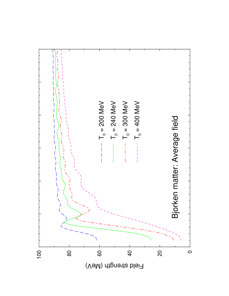
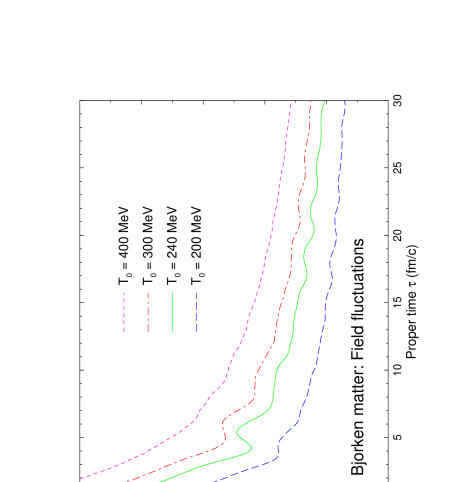
FIG. 1.: Time evolution of the field.

The time dependence of $\phi_{0}$, the magnitude of the order parameter $\phi_{0}$ (top panel), and $\delta\phi$, the associated dispersion of the field fluctuations (bottom panel), in Bjorken matter (a longitudinally expanding box) prepared at various initial temperatures, $T_{0}$, as indicated.

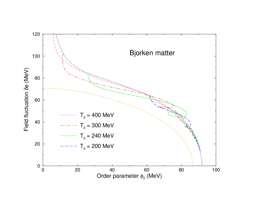
FIG. 2.: Phase evolution.

The time evolution of the expanding box is projected onto the chiral phase diagram, in which the abscissa is the order parameter $\phi_{0}$ (the magnitude of the average value of the chiral field within the box) and the ordinate is the filed fluctuation $\delta\phi$ (the dispersion in the field around its average value), for the four different initial temperatures $T_{0}$. The equilibrium path is shown by the upper dotted curve while the lower dotted curve delineates the region of instability within which the field is supercritical.

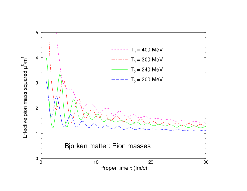
FIG. 3.: Effective mass in Bjorken matter.

The time evolution of the square of the effective pion mass, $\mu_{\pi}^{2}(t)$ (divided by the square of its free mass $m_{\pi}$) for Bjorken matter prepared at four different initial temperatures $T_{0}$ at the proper time $\tau_{0}=1~{}{\rm fm}/c$.

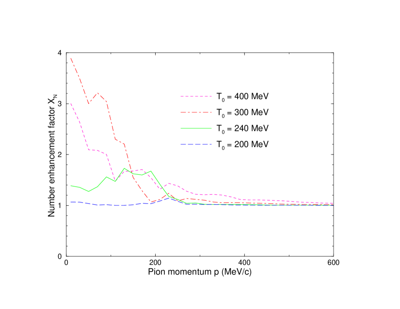
FIG. 4.: Enhancement factor.

The number enhancement coefficient $X_{N}$ obtained as described in Ref. [35] on the basis of the time dependent effective masses given in Fig. 3. The coefficient $X_{N}$ expresses the relative increase in the population of a given pion mode, as characterized by the momentum $p=\hbar kc$.

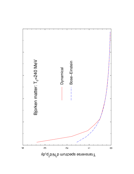
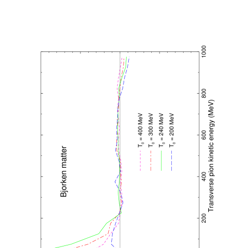
FIG. 5.: Transverse spectrum for Bjorken matter.

The top panel shows the final transverse pion spectrum, $d^{3}N/d^{2}{\mbox{\boldmath$p$}}_{\perp}d{\sf y}$, and the associated equilibrium spectrum obtained by fitting the result for the longitudinally expanding Bjorken box with a Bose-Einstein form within the energy interval 200-1000 MeV, for the initial temperature $T_{0}=240~{}{\rm MeV}$. The bottom panel shows the ratio between the dynamically generated spectrum and the fitted equilibrium form, for four different initial temperatures $T_{0}$.

FIG. 6.: The initial geometry of the Bjorken rod.

The initial field configuration describes a rod-like system subject to a longitudinal scaling expansion of the Bjorken type, for which the local boost rapidity is given by ${\sf y}=z/\tau$.

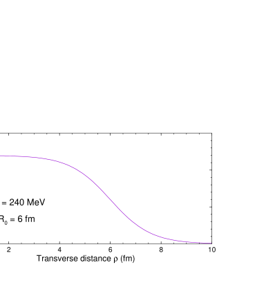
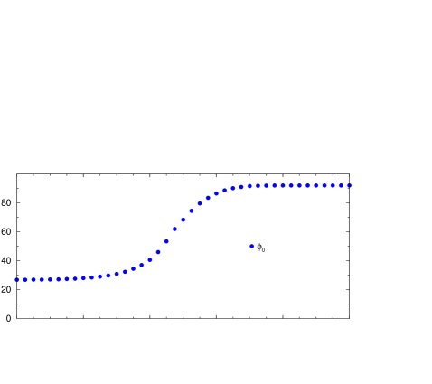
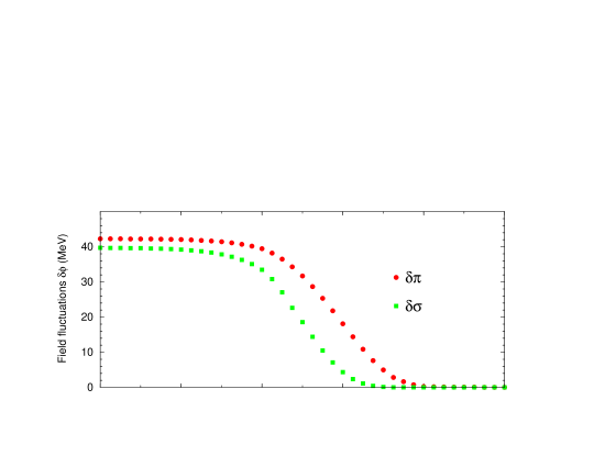
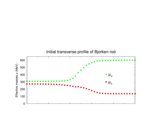
FIG. 7.: Initial rod profiles.

The transverse profiles of the local temperature $T$, the order parameter $\phi_{0}$, the mean fluctuation of the field in a given O(4) direction, $\delta\sigma$ and $\delta\pi$, and the corresponding effective masses $\mu_{\sigma}$ and $\mu_{\pi}$, for a rod with a radius of $R_{0}=6~{}{\rm fm}$ and a central temperature of $T_{0}=240~{}{\rm MeV}$.

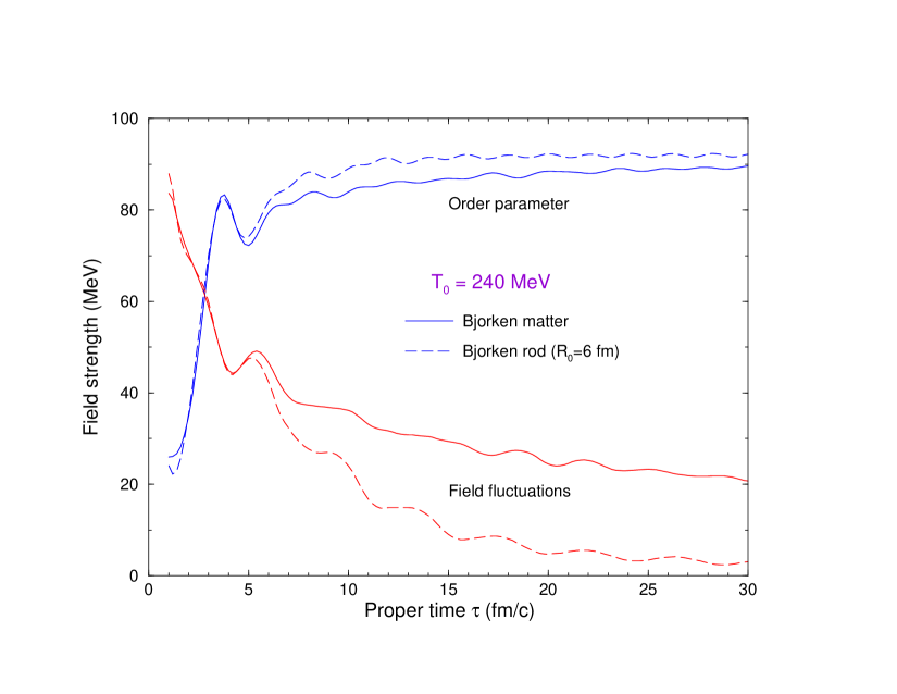
FIG. 8.: Time evolution of the field.

The time dependence of $\phi_{0}$, the magnitude of the order parameter (increasing curves), and $\delta\phi$, the associated dispersion of the field fluctuations (decreasing curves), in both Bjorken matter prepared with $T_{0}=240~{}{\rm MeV}$ (solid curves) and the corresponding Bjorken rod with $R_{0}=6~{}{\rm fm}$ (dashed curves). The information for the rod has been obtained by averaging over a hollow cylindrical volume, $1~{}{\rm fm}<\rho<3~{}{\rm fm}$. (The region very close to the symmetry axis has been excluded in order to avoid the enhanced fluctuations in the center caused by the strict axial symmetry of the geometry.)

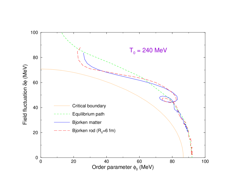
FIG. 9.: Phase evolution of the rod.

The phase evolution of the interior of the Bjorken rod prepared with a bulk temperature of $T_{0}=240~{}{\rm MeV}$ and a radius of $R_{0}=6~{}{\rm fm}$ (dashed path, filled diamonds), compared with the corresponding evolution of Bjorken matter shown in Fig. 2 (solid path, open circles). The equilibrium path is shown by the short-dashed curve while the dotted curve delineates the region of instability within which the field is supercritical. The information for the rod has been obtained by averaging over a hollow cylindrical volume, $1~{}{\rm fm}<\rho<3~{}{\rm fm}$. The symbols give the location of the paths at successive proper times $\tau=1,2,3,4,5,10,20,30~{}{\rm fm}/c$.

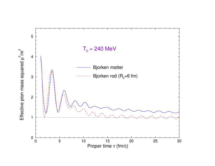
FIG. 10.: Effective mass.

The time evolution of the square of the effective pion mass, $\mu_{\pi}^{2}(t)$ (divided by the square of its free mass $m_{\pi}$) for a Bjorken rod (dashed curve) prepared with $T_{0}=240~{}{\rm MeV}$ and $R_{0}=6~{}{\rm fm}$ as well as the corresponding result for Bjorken matter taken from Fig. 3 (solid curve). The information for the rod has been obtained by averaging over a hollow cylindrical volume, $1~{}{\rm fm}<\rho<3~{}{\rm fm}$.

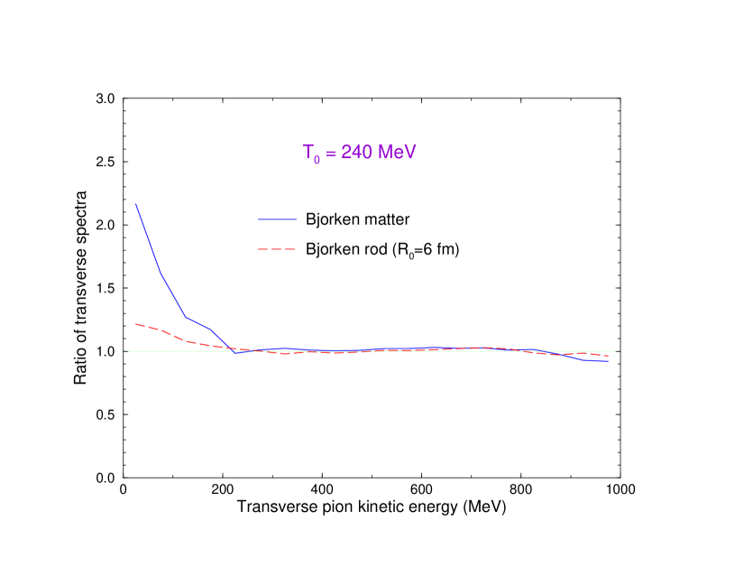
FIG. 11.: Spectral shape for Bjorken rods.

The ratio between the final transverse pion spectrum, $d^{3}N/d^{2}{\mbox{\boldmath$p$}}_{\perp}dy$, and the associated equilibrium spectrum obtained by fitting the dynamical result with a Bose-Einstein form within the energy interval 200-1000 MeV, for a longitudinally expanding rod (dashed curve) having an initial radius of $R_{0}=6~{}{\rm fm}$ and with an initial bulk temperature of $T_{0}=240~{}{\rm MeV}$, as well as the corresponding result for Bjorken matter (from Fig. 5).

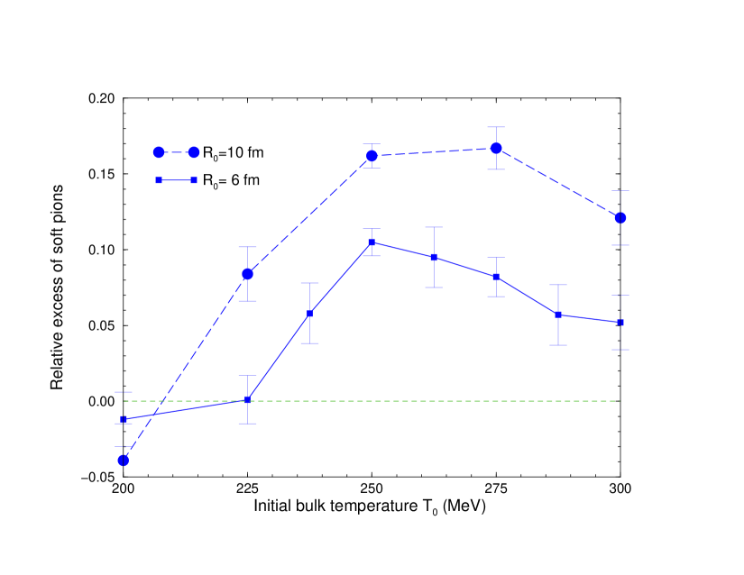
FIG. 12.: Excess of soft pions for Bjorken rods.

The relative excess of pions for Bjorken rods with initial radii $R_{0}$ equal to either 6 or 10 fm, as a function of the initial bulk temperature $T_{0}$. The excess has been obtained by subtracting the yield of pions with kinetic energies below 200 MeV from the corresponding equilibrium spectrum obtained by fitting the dynamical result with a Bose-Einstein form within 200-1000 MeV.

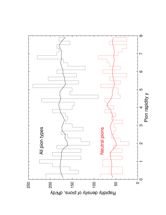
FIG. 13.: Rapidity density.

The rapidity density of pions for a single event prepared with $T_{0}=250~{}{\rm MeV}$, as obtained by dividing the number in each slice by its width $\Delta{\sf y}=0.2$. The expected multiplicity based on the calculated asymptotic field is indicated by the smooth solid curve, while the histogram shows the actual number as picked from the corresponding Poisson distributions. The top curves include all three pion types, whereas the bottom curves show the neutral pions only.

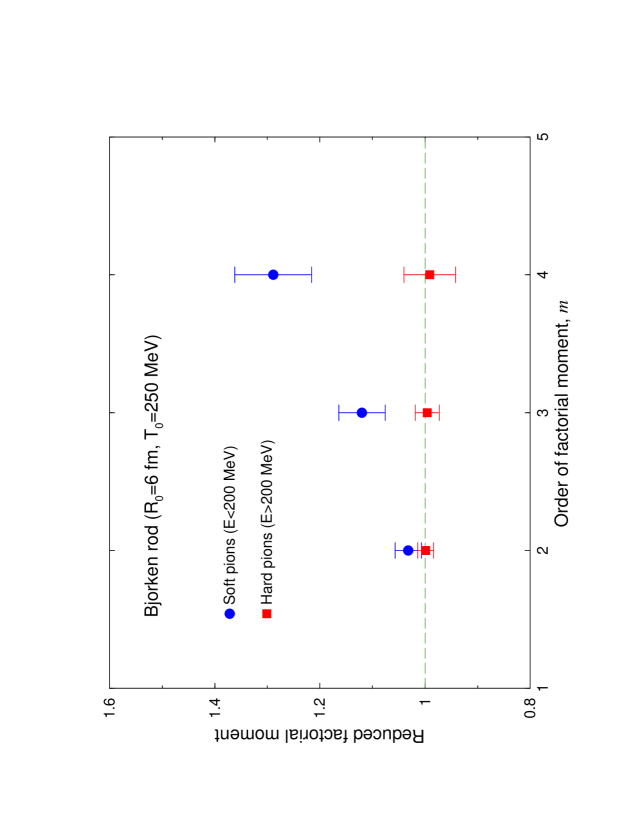
FIG. 14.: Reduced factorial moments.

The reduced factorial moments ${\cal M}_{m}/\bar{N}^{m}$ obtained for a sample of rods prepared with $R_{0}=6~{}{\rm fm}$ and $T_{0}=250~{}{\rm MeV}$ displayed as a function of the order $m$, for either soft (dots) or hard (squares) pions. The error bars arise from the sampling over all lumps and events and the points have been slightly offset for clarity.

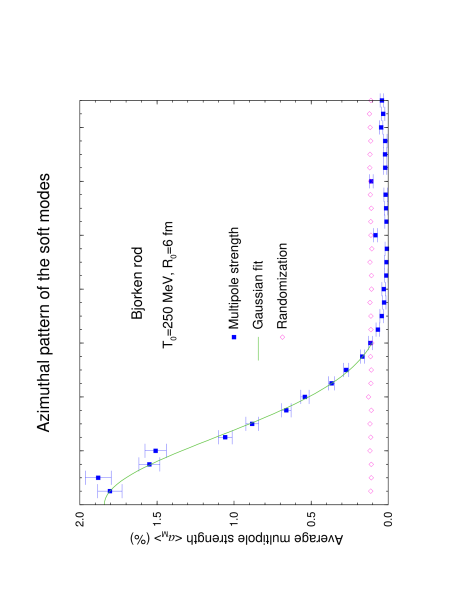
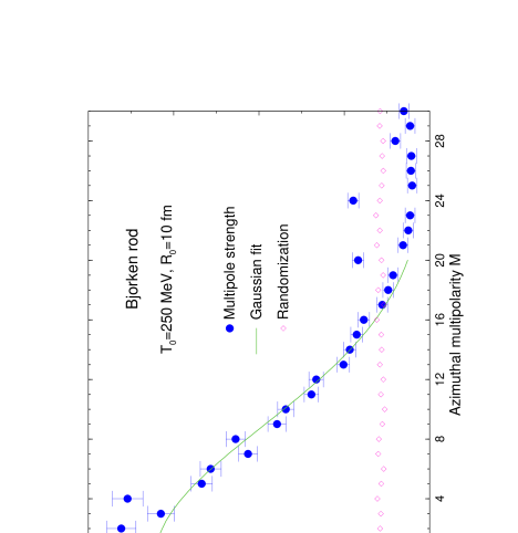
FIG. 15.: Multipole strength for soft modes.

The azimuthal multipole strength distribution (in per cent) for the soft modes of the asymptotic pion field, $\tilde{\alpha}$ (solid circles), extracted for an ensemble of events starting with an initial rod radius $R_{0}$ of either 6 or 10 fm and an initial bulk temperature of $T_{0}=250~{}{\rm MeV}$. The solid curve shows the corresponding gaussian fit. The open diamonds indicate the noise level $\tilde{\alpha}^{\rm random}_{M}$, obtained by randomizing the azimuthal direction of each pion mode before evaluating the multipole moment.

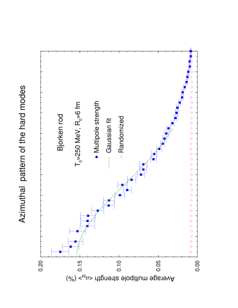
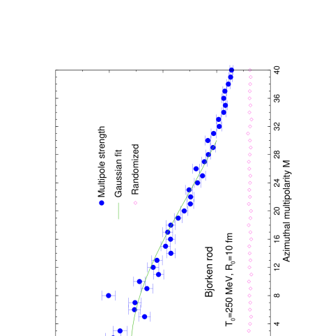
FIG. 16.: Multipole strength for hard modes.

The azimuthal multipole strength (in per cent) of the hard modes of the asymptotic pion field, $\tilde{\alpha}$, extracted for an ensemble of events starting with an initial rod radius $R_{0}$ of either 6 or 10 fm and an initial bulk temperature of $T_{0}=250~{}{\rm MeV}$, together with the corresponding gaussian fit. The open diamonds indicate the noise level $\tilde{\alpha}^{\rm random}_{M}$, obtained by randomizing the azimuthal direction of each pion mode before evaluating the multipole moment.

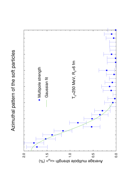
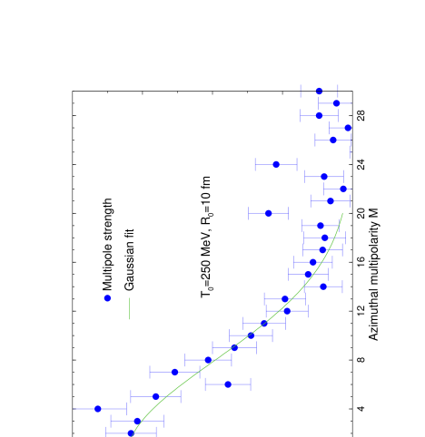
FIG. 17.: Multipole strength for soft particles.

The azimuthal moments $\alpha_{M}$ (in per cent) extracted for an ensemble of events starting with an initial rod radius $R_{0}=10~{}{\rm fm}$ and an initial bulk temperature of $T_{0}=250~{}{\rm MeV}$. These moments have been extracted from the many-particle final states obtained by sampling the actual particle numbers from the underlying asymptotic fields used in Fig. 15. The noise level averaged over the multipolarity $M$, $\langle\alpha^{\rm random}\rangle$, has been subtracted from the displayed values (they amount to 2.48 and 0.81 per cent for $R_{0}$ equal to 6 and 10 fm, respectively) and the solid curve shows the gaussian fit to the resulting difference.

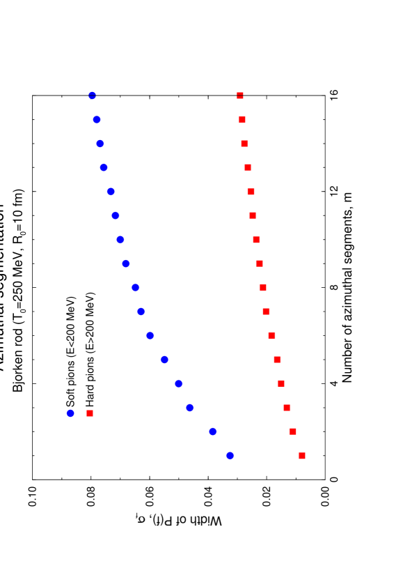
FIG. 18.: Neutral pion fraction.

The dispersion $\sigma_{f}$ of the neutral pion fraction distribution $P(f)$ for sources that have been obtained by dividing each rapidity lump into $m$ equally large azimuthal sections of width $2\pi/m$. An ensemble of rods with a initial bulk temperature $T_{0}=250~{}{\rm MeV}$ and radius $R_{0}=10~{}{\rm fm}$. The results for both soft and hard pions are shown. These moments have been extracted from the many-particle final states resulting from the underlying asymptotic fields used in Fig. 15.

REFERENCES

- [1] K. Rajagopal, Quark-Gluon Plasma 2, (Ed. R. Hwa, World Scientific, Singapore, 1995).
- [2] J.P. Blaizot and A. Krzywicki, Acta Phys. Polon. 27 (1996) 1687
- [3] J.D. Bjorken, Acta Phys. Polon. B28 (1997) 2773
- [4] A.A. Anselm, Phys. Lett. B217 (1989) 169.
- [5] A.A. Anselm and M.G. Ryskin, Phys. Lett. B266 (1991) 482.
- [6] J.D. Bjorken, K.L. Kowalski, and C.C. Taylor, SLAC-PUB-6109 (1993).
- [7] J.D. Bjorken, K.L. Kowalski, and C.C. Taylor, hep-ph/9309235.
- [8] K. Rajagopal and F. Wilczek, Nucl. Phys. B399 (1993) 395.
- [9] J.P. Blaizot and A. Krzywicki, Phys. Rev. D46 (1992) 246.
- [10] D. Boyanovsky, H.J. de Vega, R. Holman, S. Prem Kumar, Phys. Rev. D56 (1997) 5233
- [11] Z. Huang and X.-N. Wang, Phys. Lett. B383, 457 (1996).
- [12] Y. Kluger, V. Koch, J. Randrup, and X.N. Wang, Phys. Rev. C57 (1998) 280
- [13] MiniMax Collaboration (T.C. Brooks et al.), Phys. Rev. D55, 5667 (1997)
- [14] WA98 Collaboration (M.M. Aggerwal et al.), Phys. Lett. B420, 169 (1998)
- [15] K. Rajagopal and F. Wilczek, Nucl. Phys. B404 (1993) 577
- [16] J.-P. Blaizot and A. Krzywicki, Phys. Rev. D50 (1994) 442
- [17] S. Gavin, A. Gocksch, and R.D. Pisarski, Phys. Rev. Lett. 72 (1994) 2143
- [18] S. Gavin and B. Müller, Phys. Lett. B329 (1994) 486
- [19] Z. Huang and X.-N. Wang, Phys. Rev. D49 (1994) 4335
- [20] F. Cooper, Y. Kluger, E. Mottola, and J.P. Paz, Phys. Rev. D51 (1995) 2377
- [21] M. Asakawa, Z. Huang, and X.N. Wang, Phys. Rev. Lett. 74 (1995) 3126
- [22] D. Boyanovsky, H.J. de Vega, and R. Holman, Phys. Rev. D51 (1995) 734
- [23] L.P. Csernai and I.N. Mishustin, Phys. Rev. Lett. 74 (1995) 5005
- [24] S. Mrówczyński and B. Müller, Phys. Lett. 363B (1995) 1
- [25] J. Randrup, Phys. Rev. D55 (1997) 1188
- [26] F. Cooper, Y. Kluger, and E. Mottola, Phys. Rev. C54 (1996) 3298
- [27] M.A. Lampert, J.F. Dawson, and F. Cooper, Phys. Rev. D54 (1996) 2213
- [28] J. Randrup, Phys. Rev. Lett. 77 (1996) 1226
- [29] J. Randrup, Nucl. Phys. A616 (1997) 531
- [30] J.I. Kapusta and A.P. Vischer, Z. Phys. C75 (1997) 507
- [31] T.S. Biro, D. Molnar, Z.H. Feng, and L.P. Csernai, Phys. Rev. D55 (1997) 6900
- [32] G. Amelino-Camelia, J.D. Bjorken, and S.E. Larsson, Phys. Rev. D56 (1997) 6942
- [33] D. Boyanovsky, H.J. de Vega, R. Holman, S. Prem Kumar, Phys. Rev. D56 (1997) 3929
- [34] J.D. Bjorken, Phys. Rev. D27 (1983) 140
- [35] J. Randrup, Heavy Ion Phys. 9 (1999) in press; nucl-th/9907033
- [36] R.D. Pisarski, Phys. Rev. D52 (1995) R3773
- [37] A.M. Poskanzer and S.A. Voloshin, Phys. Rev. C58 (1998) 1671
- [38] J. Randrup and R.L. Thews, Phys. Rev. D56 (1997) 4392
- [39] J. Schaffner-Bielich and J. Randrup, Phys. Rev. C59 (1999) 3329
- [40] J. Randrup, Nuclear Matter in Different Phases and Transitions, Ed. J.P. Blaizot, X. Campi, and M. Ploszajczak, Kluwer Academic Publishers (Boston, 1999) p. 107