Space-time analysis: HBT at SPS and RHIC

Abstract

In this review talk, I first summarize the conclusions which can be drawn from a particle interferometric analysis of CERN SPS data and then I address related questions which are relevant for the upcoming experiments at RHIC.

1 Introduction

The CERN SPS lead beam program has covered for the first time with high statistics all HBT radius parameters of the full three-dimensional parametrization over a wide region in rapidity and transverse momentum (for data, see Ref. [1]). Theory provides by now a detailed data analysis strategy and interpretation (for a review, see Ref. [2]) . In this talk, I summarize the conclusions which we can draw from the recent CERN SPS data, and I identify questions which can be settled by the upcoming RHIC experiments.

The main goal of HBT is to determine the geometry and dynamics of the heavy ion collision at freeze-out. This information is becoming increasingly important for the discussion of other observables. For example: i) In studies of anisotropic flow [3, 4], one aims at exploiting the HBT space-time picture to disentangle geometrical and dynamical components of anisotropy [5, 6, 7, 8]. These cannot be separated on the basis of one-particle spectra alone. ii) In the search for event by event multiplicity fluctuations of qualitatively new origin (e.g. DCCs), fluctuations due to Bose-Einstein correlations are an important background source [9]. Their calculation depends strongly on the phase-space density attained in the last stage of the collision. The HBT analysis of experimental data now provides estimates of this phase space density for a large variety of collision systems [10], and work on its consequences for multiplicity fluctuations is in progress [11]. iii) In event generator studies, HBT measurements provide constraints on the simulated space-time structure [12], and the question how microscopic dynamics can account for the observed final state emission region becomes of the utmost importance.

In the light of these rapidly developing applications, one should not forget the fundamental limitations of any particle interferometric analysis. HBT extracts the phase space density $S(x,K)$ from a combination of hadronic one-particle and identical two-particle spectra of the abundant hadron species:

$$E{dN\over d^{3}p} = \int d^{4}x\,S(x,p)\,,$$ (1)

$$C({\bf K},{\bf q}) = 1+{{|\int d^{4}x\,e^{iq\cdot x}S(x,K)|^{2}}\over{\int d^{4}x\,S(x,P_{1})\,\int d^{4}y\,S(y,P_{2})}}\,.$$ (2)

However: i) $S(x,K)$ characterizes the geometry and dynamics of the collision at freeze-out and thus provides only a snapshot of the last stage of the collision. What is characterized is the result of a dynamical evolution, not the dynamical evolution itself. ii) HBT measures the relative distance between emission points. It does not measure the absolute position of emission points. This is of particular importance for the interpretation of the average emission time $\tau_{0}$, see below. iii) The measurement of $C(K,q)$ gives independent access to only three of the four space-time dependencies of $S(x,K)$. This is a consequence of detecting on-shell particles. It implies a model-dependent analysis strategy in which a model emission function $S(x,K)$ is compared to data.

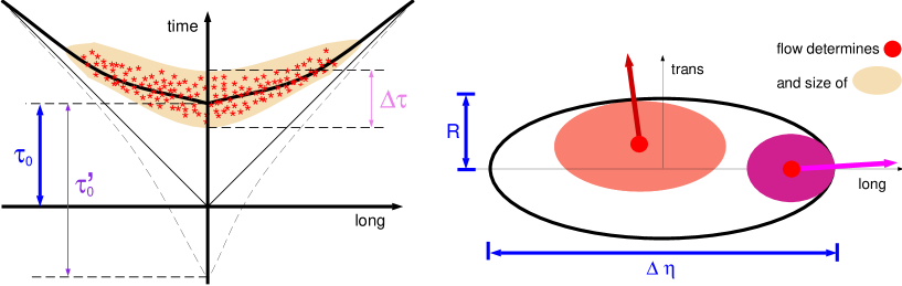
Figure 1: Characterization of the pion emission function (3) in terms of Gaussian widths $R$, $\Delta\eta$, $\Delta\tau$. The strength of the collective flow field $u_{\mu}$ determines the correlation between points of highest emissivity and predominant emission direction. The temperature $T$ determines the degree of thermal smearing around these points of highest emissivity.

2 Final State Geometry and Dynamics of Pb+Pb at 158 GeV/c

The expression for the one-particle and two-particle spectra (1) and (2) in terms of the emission function $S(x,K)$ form the starting point for various different approaches: i) In hydrodynamical simulations of heavy ion collisions [13, 14], they specify the integrations over the freeze-out hypersurface. ii) For event generator studies, a discretized formulation exists [12]. iii) Analytical model studies start from a simple parametrization of the model emission function $S(x,K)$ whose model parameters are then extracted from a fit of (1) and (2) to data. A simple, frequently used model ansatz for the phase space distribution $S(x,K)$ in terms of very few, physically intuitive fit parameters, is e.g.

$$S(x,P) = \textstyle{2J+1\over(2\pi)^{3}}\,P{\cdot}n(x)\,\exp{\left(-{P\cdot u(x)\over T}\right)}\,\exp\left(-{r^{2}\over 2R^{2}}-{\eta^{2}\over 2(\Delta\eta)^{2}}-{(\tau-\tau_{0})^{2}\over 2(\Delta\tau)^{2}}\right)\,.$$ (3)

The physics contained in this ansatz is described elsewhere in much detail [2]. As shown in the sketch of Fig. 1, the spatial extension of the pion emission region is characterized by Gaussian widths $R$, $\Delta\eta$ and $\Delta\tau$ in the transverse, longitudinal and temporal direction respectively. The absolute source position in the Minkowski diagram is fixed by the time scale $\tau_{0}$, and the pion source emits particles at temperature $T$. The model allows for a directed dynamical component via the flow field $u_{\mu}(x)$ which is assumed to show Bjorken scaling in the longitudinal direction superimposed with a transverse flow component $\sinh\eta_{t}(r)$, $\eta_{t}(r)=\eta_{f}r/R$. To sum up: the phase space density (3) is characterized by only 6 physically intuitive fit parameters: $T$, $\eta_{f}$, $R$, $\Delta\eta$, $\Delta\tau$ and $\tau_{0}$.

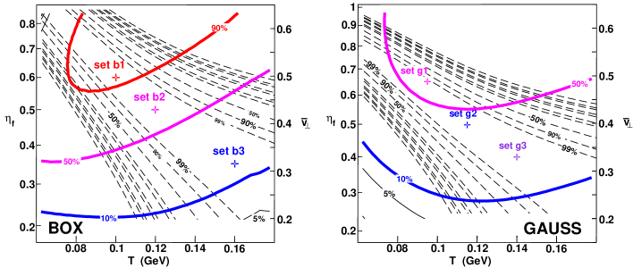
Figure 2: Confidence levels for the optimal temperature $T$ and transverse flow $\eta_{f}$ values from fits of particle emission functions to NA49 one-particle spectra (dashed lines) and two-particle spectra (solid lines). The transverse density profile of model emission functions was chosen box-shaped (l.h.s.) and Gaussian (r.h.s.). Figure from Ref. [23].

Studies of many modifications of the parametrization (3) exist. These include e.g. the effects of resonance decay contributions [15], other flow profiles [16], temperature gradients [17, 18], source opacity [19] and azimuthal asymmetries [6]. Comparisons of the particular model (3) with experimental data exist for AGS [20] and SPS [21, 22] energies. The main argument in favour of a largely model-independent interpretation of the model parameters extracted in these studies is that the measured particle spectra (1) and (2) are mainly sensitive to the various r.m.s. of the emission function and depend only weakly on the particular analytical implementation. What matters is mainly the average transverse flow and the r.m.s. width of the transverse density profile, not their particular $r$-dependence. A recent analysis [23] of NA49 data indicates the limitations to these statements:

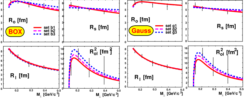
Figure 3: Comparison of the NA49 Pb+Pb HBT radius parameters at mid rapidity ($h^{+}\,h^{+}$ and $h^{-}\,h^{-}$ data are averaged) to results from model emission functions with box-shaped (l.h.s.) and Gaussian (r.h.s.) density profile. Different curves indicate the parameter sets shown in Fig. 2. Figure taken from [23].

B. Tomášik [23] has compared the model emission function (3) to a model in which the Gaussian transverse density distribution of (3) was replaced by a box-shaped one, $\exp\left(-{r^{2}\over 2\,R_{G}}\right)\longrightarrow\Theta(r-R_{B})$. For a comparison of the determined fit parameters of both models, one averages the transverse flow over the transverse density profile $H_{\rm profile}(r)$ and one recalls that the r.m.s. width for a Gaussian and a box profile differs by a factor 2:

$$\overline{v}_{\perp} = {1\over{\cal N}}\int r\,dr\,\tanh(\eta_{t}(r))\,H_{\rm profile}(r)\,,$$ (4)

$$r_{\rm rms} = \sqrt{2}\,R_{G}=\textstyle{1\over\sqrt{2}}R_{B}\,,\qquad\eta_{t}(r)=\eta_{f}\textstyle{r\over r_{\rm rms}}\,.$$ (5)

The slope of the transverse one-particle spectrum is due to a combination of random (thermal) and directed (flow) transverse motion. Different combinations of temperature $T$ and transverse flow $\eta_{f}$ lead to the same effective blue-shifted temperature. As seen in Fig. 2, the parameter combinations favoured by the fit specify a sharp valley in the $T-\eta_{f}$-plane. The contour plots in this figure are similar for a Gaussian and box-shaped density distribution, but they are not identical. The reason is that for an $r$-dependent flow field, particle emission from different transverse distances $r$ occurs with different average transverse momentum. Modifying the transverse density profile $H_{\rm profile}(r)$ can thus affect the $p_{t}$-dependence of the transverse one-particle spectrum. For the low-$p_{t}$ region ($p_{t}<1.5$ GeV) measured by NA49, these model-dependent variations are seen to be small. However, the high $p_{t}$ tails of the measured spectrum test in these analytical models the large $r$-tails of the distribution $H_{\rm profile}(r)$ which is almost unconstrained by other observables. An application of these models to higher $p_{t}$ (see e.g. Ref. [24]) may hence be expected to emphasize the model-specific $r$-dependence of $H_{\rm profile}(r)$ and $\eta_{t}(r)$. The model-dependence increases with $p_{t}$ - this is an important message for similar studies at RHIC.

HBT correlation radii allow to disentangle the $T-\eta_{f}$ ambiguity of the fit to the one-particle spectrum. This is seen from the contour plot of Fig. 2. The contours for the 90, 50 and 10 % confidence levels are still very wide due to current experimental uncertainties, but they clearly show a different $T-\eta_{f}$ correlation. The fit favours a box-shaped density profile over a Gaussian one. The parameter sets indicated by $b1$, $b2$, $b3$ and $g1$, $g2$, $g3$ in Fig. 2 are used as input for the fits to the HBT radii in Fig. 3. In the $T-\eta_{f}$ plane, the fit is driven by the slope of the side and out radius parameters, and the preferred values thus depend strongly on taking all contributions to this slope properly into account. All existing data analyses [20, 21, 22, 23] favour relatively low temperatures and large transverse flows.

The values [23] of the model parameters used for the fits of Fig. 3 are summarized in the table at the end of this section. The box-shaped and Gaussian model emission functions differ in several details. Especially, a box-shaped density profile reproduces the data with better $\chi^{2}$. A similar trend was also pointed out in a recent study of deuteron coalescence models [25]. But irrespective of these finer tendencies in the data, the main message is unaffected by details of the analytical form of the emission function: we observe a system with strong transverse flow which has expanded up to freeze-out to twice its initial size, and which has cooled down substantially during this expansion.

It is an important problem to understand the dynamical origin of these source characteristics. One may e.g. question the dynamical consistency of the presented data on the ground that the average transverse velocity $\bar{v}_{\perp}$ and the emission time $\tau_{0}$ seem barely enough to account for an expansion to twice the initial size. However, HBT does not measure absolute positions, and the model parameter $\tau_{0}$ thus provides only a lower bound for the total time after impact [2]. Also, very little is known about the question how fast the final transverse flow of a hadronic system can be built up during the collision. At present, one cannot even rule out the point of view that without novel dynamical assumptions, none of the existing event generators can account for the observed strong transverse expansion solely with final state interactions [26].

A constructive first step to clarify the dynamical origin of HBT fit parameters is the comparison of HBT radii from event generators and experiment combined with a comparison of the simulated space-time structure to the model (3). This may help to understand how a dynamical model in which the time after impact is known can account for the measured data.

	box-shaped			Gaussian
set	b1	b2	b3	g1	g2	g3
$T$ (MeV)	100	120	160	100	120	160
$\eta_{f}$	0.6	0.5	0.35	0.6	0.48	0.35
$R_{B}/R_{G}$ (fm)	$12.1\pm 0.2$	$11.5\pm 0.2$	$10.7\pm 0.2$	$6.5\pm 0.1$	$5.9\pm 0.2$	$5.6\pm 0.1$
$\tau_{0}$ (fm/$c$)	$6.3\pm 1.1$	$5.5\pm 1.1$	$4.4\pm 3.5$	$7.8\pm 0.8$	$6.6\pm 0.9$	$5.5\pm 0.9$
$\Delta\tau$ (fm/$c$)	$3.6\pm 0.6$	$3.2\pm 0.7$	$2.6\pm 2.0$	$2.3\pm 0.7$	$2.3\pm 0.7$	$1.8\pm 0.8$
$\Delta\eta$ (fixed)	1.3	1.3	1.3	1.3	1.3	1.3
$\bar{v}_{\perp}$	0.5	0.43	0.33	0.46	0.39	0.29

3 Phase space density

Once the emission function $S(x,K)$ is determined, the particle phase space density $f({\bf x},{\bf p},t)$ is obtained by integrating $S(x,K)$ over all particles emitted up to the time $t$, [2]. Of particular interest is the spatially averaged phase space density $\langle f\rangle({\bf K})$ which is directly related to the measured particle spectra [27, 28, 10]:

$$\langle f\rangle({\bf K})={{\int d^{3}x\,f^{2}({\bf x},{\bf K},t>t_{f})}\over\int d^{3}x\,f({\bf x},{\bf K},t>t_{f})}={dN\over dY\,M_{\perp}\,dM_{\perp}\,d\Phi}\,{\sqrt{\lambda(K_{\perp},Y)}\over V_{\rm eff}(K_{\perp},Y)}\,.$$ (6)

This is a measure for the number of particles in a momentum bin $dY\,M_{\perp}\,dM_{\perp}\,d\Phi$ which are contained inside the spatial volume $V_{\rm eff}(K_{\perp},Y)$. The spatial volume $V_{\rm eff}(K_{\perp},Y)$ is determined by the measured HBT radius parameters:

$$V_{\rm eff}(K_{\perp},Y)={{M_{\perp}\,\cosh Y}\over\pi^{3/2}}\,\left(R_{s}\,\sqrt{R_{0}^{2}\,R_{l}^{2}-(R_{ol}^{2})^{2}}\right)\,.$$ (7)

The $\lambda$ intercept parameter in (6) ensures that pions from long-lived resonance decay contributions [15], which are emitted outside the collision region, do not contribute to the average phase space density $\langle f\rangle({\bf K})$.

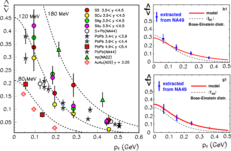
Figure 4: Spatially average phase space density in narrow rapidity windows as a function of the transverse momentum. Dashed lines denote Bose-Einstein distributions at temperatures $T=$ 80, 120 and 180 MeV. Figure from  [10] (l.h.s.) and  [23] (r.h.s.).

With the help of (6), D. Miskowiec found in the E877 data a factor 2 decrease of the phase space density in the very forward rapidity region. A comprehensive analysis [10] of various different collision systems reveals now that such strong rapidity variations of $\langle f\rangle({\bf K})$ occur only very close to the kinematically allowed boundaries. As seen from Fig. 4, except for the projectile rapidity region, $\langle f\rangle({\bf K})$ is almost universal. The variation of $\langle f\rangle({\bf K})$ is small compared to the order of magnitude change in the $dN^{-}/dY$ between the different collision systems (22 for S-S vs. 185 for Pb-Pb). The transverse momentum dependence of $\langle f\rangle({\bf K})$ is in rough agreement with a Bose-Einstein distribution. Deviations from this show up in a weaker transverse momentum dependence of $\langle f\rangle({\bf K})$ and can be accounted for by transverse flow. This is seen on the r.h.s. of Fig. 4, where the average phase space density extracted from NA49 mid rapidity data is compared to results from the optimal model parameter sets ’b1’ and ’g1’ indicated in Fig. 2.

4 Extrapolation of the AGS and SPS systematics to RHIC

All observations indicate that the decoupling of pions occurs at an approximately constant phase space density irrespective of the collision system. This implies that the freeze-out volume scales with particle multiplicity

$$V_{\rm eff}(K_{\perp},Y)\propto{dN^{-}\over dY\,M_{\perp}\,dM_{\perp}\,d\Phi}\,.$$ (8)

The qualitatively new aspect of Fig. 4 is to establish equation (8) differentially, i.e. for narrow bins in transverse momentum and rapidity. $K_{\perp}$-integrated versions of (8) are well-known. NA35 observed e.g. for different collision systems a linear increase of the $K_{\perp}$-averaged collision volume with $dN^{-}/dY$ up to $dN^{-}/dY=60$  [29]. The $K_{\perp}$-averaged NA49 data for central rapidity follows the same systematics up to $dN^{-}/dY=180$, and RHIC will allow to test this systematics even further.

Eq. (8) can be used for extrapolation into this new high multiplicity regime accessible to RHIC: The most naive RHIC-prediction is obtained by turning $V_{\rm eff}\propto dN/dY$ into a simple multiplicity dependence for the side radius parameter which is typically the least affected by the dynamics, $R_{s}\propto\left(dN/dY\right)^{1/3}$. This leads to $R_{s}\approx 9$ fm for ${dN^{-}\over dY}=600$ and $R_{s}\approx 11$ fm for ${dN^{-}\over dY}=1200$. Depending on the dynamics, however, even if (8) holds, the transverse radius parameters may be larger or smaller. One such example, based on a hydrodynamical picture, assumes that the transverse flow gradient does not change between heavy ion collisions at SPS and RHIC. From this picture, one expects changes in the emission time $\tau_{0}$, transverse radius $R$, and transverse flow $\eta_{f}$ [30]

$$\tau_{0}\Bigg{|}_{\rm RHIC}\approx 2\,\tau_{0}\Bigg{|}_{\rm SPS}\,,\qquad\quad R\Bigg{|}_{\rm RHIC}\approx 1.3\,R\Bigg{|}_{\rm SPS}\,,\qquad\quad\eta_{f}\Bigg{|}_{\rm RHIC}\approx 1.3\,\eta_{f}\Bigg{|}_{\rm SPS}\,.$$ (9)

The resulting HBT radius parameters indicate a collision system which is substantially more extended along the beam axis at the expense of a relatively small increase in the transverse extensions,

$$R_{s}|^{\rm RHIC}\leq 1.2R_{s}|^{\rm SPS}<8\quad\hbox{\rm fm}\,,\qquad\quad R_{\parallel}|^{\rm RHIC}\approx 2R_{\parallel}|^{\rm SPS}\,.$$ (10)

Most scenarios favour a sudden bulk freeze-out of all pions which is reflected in small values for $R_{o}^{2}-R_{s}^{2}$. However, hydrodynamical scenarios with a particularly soft equation of state lead to large differences between the two transverse parameters [31]: $R_{o}^{2}\gg R_{s}^{2}$. In these scenarios, only $\approx 50$ percent of the difference $R_{o}^{2}-R_{s}^{2}$ stems from an extended lifetime of the system. An equally important contribution to $R_{o}^{2}-R_{s}^{2}$ comes from a strong negative $x$-$t$ correlation [14].

5 Multiparticle Bose-Einstein symmetrization

Standard calculations of the two-particle correlator $C(K,q)$ are based on approximating $N$-particle symmetrized final state wavefunction by a sum of two-particle symmetrized contributions. For small phase space densities, this is a valid approximation. However, if the phase space density is sufficiently high, multiparticle symmetrization effects cannot be ignored. Recently, progress was made in quantifying the decisive words ”sufficiently high” of this last sentence in simple model studies:

The well-known combinatorial problem is that one obtains from an $N$-particle symmetrized wavefunction $N!$ contributions to the measurable particle spectra. Even for moderate event multiplicities, brute force numerical calculation do not work ($100!\approx 9*10^{157}$). However, for pion emitting sources defined by the emission function $S(x,K)$ and the event multiplicity $N$, Pratt’s algorithm [9] provides a substantial simplification:

Here, the building blocks $G_{n}({\bf p}_{i})$, $C_{n}$ and $w(n)$ are defined in terms of $n$-dimensional integrals over $S(x,K)$, $n\leq N$. All measured spectra reduce to sums over products of these building blocks. While the technicalities of this approach cannot be explained shortly (see Ref. [2] for a review), the important message is that the sums involved in the final answer run over the number of all partitions of $N$ different contributions, rather than over $N!$. Note that Partitions[N=100] =$2*10^{9}$, and this makes a numerical calculation feasible.

The remaining computational task is the calculation of the $n$-dimensional integrals $G_{n}$, $C_{n}$ and $w(n)$. For Gaussian emission functions, this can be done analytically [32, 33]. Fig. 5 shows the results of such a model study and confirms the observations of Zajc [34]. Pions like to sit close together in momentum space and this leads to a steepening of the one-particle spectrum. Also, they like to sit close together in configuration space and hence the two-particle correlator gets wider. As can be seen from Fig. 5, these effects are small but visible for realistic phase space densities below $1\,\,\hbar^{3}$.

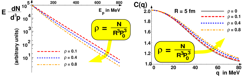
Figure 5: Modifications of one-particle spectrum (l.h.s.) and two-particle correlator (r.h.s.) due to multiparticle symmetrization effects. With increasing phase space density, the one-particle spectrum gets steeper and the two-particle spectrum gets wider. Figure taken from [33].

However, existing calculations like Fig. 5 cannot be compared to experiment. The problem is that despite some recent progress [35], there is no realistic description of multiparticle final state Coulomb interactions. The HBT effect and Coulomb repulsion occur both on the same relative momentum scale and counteract each other. One may hence expect that their multiparticle contributions cancel to a large extent. Thus, present calculations can be expected to provide a loose upper bound on multiparticle symmetrization effects. The important message for RHIC is that if the so far universal value of $\langle f\rangle({\bf K})$ is confirmed at RHIC, multiparticle effects to the momentum spectra are of minor importance.

6 Multiplicity fluctuations

There is one important observable where the calculation of multiparticle symmetrization effects allows for a comparison with experimental data and that is the modification of the charged to neutral multiplicity distribution due to Bose-Einstein statistics. A typical Bose-Einstein modified distribution, proposed originally for the description of anomalous cosmic ray (CENTAURO) events, is [36]

$$P(n_{0},n_{+},n_{-})={1\over Z}\,{N!\over 3^{N}}\,{w(n_{0})\over n_{0}!}\,{w(n_{+})\over n_{+}!}\,{w(n_{-})\over n_{-}!}\,\Bigg{|}_{N=\sum n_{i}}\,.$$ (11)

Here, the total number $N$ of neutral and charged pions is kept constant, but one assumes that the multiplicity distribution is arranged according to BE-statistics via the channel $\pi^{0}\,\pi^{0}$ $-$ $\pi^{+}\,\pi^{-}$. $Z$ is a normalization, and $w(n)$ denotes the multiparticle symmetrization weights which include higher order correlations. According to Pratt’s formalism, they are given by a sum over all partitions $(m,l_{m})_{n}$ of the building blocks $C_{m}$ [9]

$$w(n)=\sum_{(m,l_{m})_{n}}{C_{1}^{l_{1}}\,C_{2}^{l_{2}}\,\cdots\,C_{m}^{l_{m}}\over{\prod_{m}\,m^{l_{m}}\,(l_{m}!)}}$$ (12)

These expressions simplify substantially for Gaussian models of the emission function $S(x,K)$. One observes that the leading contribution to the building blocks $C_{m}$ is a simple polynomical in the phase space volume $\epsilon$ [33],

$$C_{m}\approx\epsilon^{m-1}\,,\qquad\hbox{where}\qquad\epsilon={\hbar^{3}\over R^{3}\,P_{0}^{3}}\,,$$ (13)

and this reduces the complicated combinatorics of (12) to a simple polynomial [33]

$$w(n)=\prod_{k=1}^{n}\bigl{(}1+\epsilon(k-1)\bigr{)}\,.$$ (14)

Based on equations (11) - (14), P. Steinberg [11] has studied the charged to neutral particle ratio measured by WA98. He starts from the observation that the distribution of this ratio is approximately 15 % broader than that obtained in a VENUS 4.12 event generator simulation. Clearly, this discrepancy can have many reasons. The strong working hypothesis in Ref. [11] is that the event generator describes the physics correctly but misses multiparticle symmetrization effects (as all Monte Carlo models do). As a remedy of the latter, the VENUS 4.12 multiplicity distribution was modified via (11). P. Steinberg finds that for phase space densities consistent with those shown in Fig. 4, multiparticle correlations can account for a substantial part of the observed discrepancy (approx. 8-10 %). Irrespective of the real origin of the discrepancy, this is a remarkable result: even for the relatively small measured phase-space densities, Bose-Einstein statistics leads to visible changes in multiplicity distributions. This also indicates that Bose-Einstein correlations are an important background source in searches of qualitatively new physics (e.g. DCCs) in multiplicity distributions.

I thank U. Heinz, J.G. Cramer, D. Ferenc and B. Tomášik with whom I had the privilege to collaborate. This work was sponsored by DOE Contract No. De-FG-02-92ER-40764.

References

- [1] NA49 Coll., H. Appelshäuser et al., Eur. Phys. J. C 2 (1998) 661.
- [2] U.A. Wiedemann and U. Heinz, nucl-th/9901094, Phys. Rep. in press.
- [3] J.-Y. Ollitrault, Nucl. Phys. A638 (1998) 195c.
- [4] A.M. Poskanzer and S.A. Voloshin, Phys. Rev. C 58 (1998) 1671.
- [5] S.A. Voloshin and W.E. Cleland, Phys. Rev. C 53 (1996) 896; ibid. 54 (1996) 3212.
- [6] U.A. Wiedemann, Phys. Rev. C 57 (1998) 266.
- [7] H. Heiselberg, Phys. Rev. Lett. 82 (1999) 2052.
- [8] D. Teaney and E.V. Shuryak, nucl-th/9904006.
- [9] S. Pratt, Phys. Lett. B301 (1993) 159; and Phys. Rev. C 50 (1994) 469.
- [10] D. Ferenc et al., hep-ph/9902342, Phys. Lett. B in press.
- [11] P. Steinberg, Proceedings for the Relativistic Heavy Ion Symposium - APS Centennial, 26 March 1999, to be published by World Scientific.
- [12] K. Geiger, J. Ellis, U. Heinz and U.A. Wiedemann, hep-ph/9811270.
- [13] B.R. Schlei, D. Strottman, J.P. Sullivan and H.W. van Hecke, nucl-th/9809070.
- [14] S. Bernard, D. Rischke, J. Maruhn and W. Greiner, Nucl. Phys. A625 (1997) 473.
- [15] U.A. Wiedemann and U. Heinz, Phys. Rev. C 56 (1997) 3265.
- [16] U.A. Wiedemann, P. Scotto and U. Heinz, Phys. Rev. C 53 (1996) 918.
- [17] T. Csörgő and B. Lörstad, Phys. Rev. C 54 (1996) 1396.
- [18] B. Tomášik and U. Heinz, Eur. Phys. J. C 4 (1998) 327.
- [19] H. Heiselberg and A. Vischer, Eur. Phys. J. C 1 (1998) 593; Phys. Lett. B421 (1998) 18.
- [20] S. Chapman and J.R. Nix, Phys. Rev. C 54 (1996) 866.
- [21] U.A. Wiedemann, B. Tomášik and U. Heinz, Nucl. Phys. A638 (1998) 475c.
- [22] G. Roland et al. (NA49 Coll.), Nucl. Phys. A638 (1998) 91c.
- [23] B. Tomášik, PhD-thesis, Universität Regensburg, January 1999.
- [24] WA98 Coll., M.M. Aggarwal et al., nucl-ex/9901009.
- [25] R. Scheibl and U. Heinz, Phys. Rev. C59 (1999) 1585.
- [26] M. Gyulassy, private communication.
- [27] G.F. Bertsch, Phys. Rev. Lett. 72 (1994) 2349; ibid. 77 (1996) 789(E).
- [28] D. Miśkowiec et al. (E877 Coll.), Nucl. Phys. A610 (1996) 227c.
- [29] T. Alber et al. (NA35 Coll.), Zeit. Phys. C66 (1995) 77.
- [30] U. Heinz, talk at the LBNL RHIC Winter Workshop, 8. Jan. 99.
- [31] D. Rischke and M. Gyulassy, Nucl.Phys. A608 (1996) 479.
- [32] T. Csörgő and J. Zimányi, Phys. Rev. Lett. 80 (1998) 916.
- [33] U.A. Wiedemann, Phys. Rev. C 57 (1998) 3324.
- [34] W.A. Zajc, Phys. Rev. D 35 (1987) 3396.
- [35] H.W. Barz, Phys. Rev. C 53 (1996) 2536.
- [36] S. Pratt and V. Zelevinsky, Phys. Rev. Lett. 72 (1994) 816.