[

Baryon Fluctuations in High Energy Nuclear Collisions

Abstract

We propose that dramatic changes in the variances and covariance of protons and antiprotons can result if baryons approach chemical equilibrium in nuclear collisions at RHIC. To explore how equilibration alters these fluctuations, we formulate both equilibrium and nonequilibrium hadrochemical descriptions of baryon evolution. Contributions to fluctuations from impact parameter averaging and finite acceptance in nuclear collisions are numerically simulated.

]

Event-by-event fluctuations of the particle yields in relativistic nuclear collisions can be sensitive to the degree of chemical equilibration [1] and to critical fluctuations due to the QCD phase transition [2, 3]. We study for the first time the degree to which chemical equilibration can affect the fluctuations of baryons at RHIC and LHC. Baryons and antibaryons are likely produced in such abundance that event-by-event yields can be measured [4]. We propose that chemical equilibration can appreciably change the variances and covariance of protons and antiprotons compared to thermal and participant-nucleon model expectations.

Fluctuations of the baryon-antibaryon system can vary depending on the degree to which the chemical reactions $N\overline{N}\leftrightarrow$ mesons reach equilibrium [4]. In the absence of chemical equilibrium, the number of antibaryons and baryons are independently conserved. Fluctuations of the particle number are then Poissonian,

$${\cal V}\equiv\sum_{i}(N_{i}-\langle N\rangle)^{2}\approx N,\,\,\,\,\,\,\,\,\,\,\,\,\,\,\,\,{\rm thermal}$$ (1)

where $N_{i}$ is the baryon number in the $i^{\rm th}$ event and $N\equiv\langle N\rangle$ is the event average. HIJING and similar participant nucleon models exhibit essentially the same behavior for nucleus-nucleus collisions [3]. In contrast, chemical equilibrium relates fluctuations of the baryons to those of the antibaryons, reducing the relative variance compared to (1). We find [4]:

$${\cal V}\approx N^{2}(N+\overline{N})^{-1},\,\,\,\,\,\,\,\,\,\,{\rm chemical}$$ (2)

where $\overline{N}$ is the average number of antibaryons. We recover (1) in the limit $N\gg\overline{N}$, since baryon conservation fixes the number of particles in that limit.

If chemical equilibrium is achieved in RHIC collisions, the variance (2) can fall to half the thermal and participant-nucleon model level, because the numbers of baryons and antibaryons are expected to be comparable at midrapidity [5]. We propose that a further signal of equilibration can be obtained from the baryon-antibaryon covariance,

$${\cal C}=\sum_{i}(\overline{N}_{i}-\langle\overline{N}\rangle)(N_{i}-\langle N\rangle).$$ (3)

In chemical equilibrium, we find that the covariance can be negative,

$${\cal C}\approx-N\overline{N}(N+\overline{N})^{-1}.\,\,\,\,\,\,\,\,\,\,{\rm chemical}$$ (4)

On the other hand, this quantity essentially vanishes for collisions of large nuclei in thermal equilibrium, or when $N\gg\overline{N}$.

The anti-correlation (4) seems somewhat surprising – positive correlations between baryons and antibaryons are seen in $e^{+}e^{-}$ experiments [6] and incorporated, e.g., in string fragmentation models [7]. Such correlations are required by baryon number conservation for those comparatively small systems. In contrast, the anti-correlation (4) and the reduction of the variance (2) result from fluctuations of the net baryon number itself. In a subvolume of a large system, fluctuations can increase the net baryon number $N_{B}$ if either a particle enters or an antiparticle exits the subvolume. Correspondingly, fluctuations of $N_{B}$ simultaneously increase $N$ and reduce $\overline{N}$, leading to an anti-correlation. This effect is only possible if chemical reactions render the individual numbers $N$ and $\overline{N}$ indefinite.

To determine the degree of chemical equilibration from fluctuations in experiments, one must account for the following additional sources of fluctuations, all of which tend to increase $\cal V$ and drive $\cal C$ toward positive values. Near local equilibrium, thermal and volume fluctuations produce particle number fluctuations. In experiments, further fluctuations result from centrality selection and detector acceptance effects [4, 3]. To illustrate how volume and thermal fluctuations can change the variance of particle yields, we begin by extending the thermodynamic formulation of ref. [4]. We then apply the Monte Carlo event generator of [4] to compute the experimental contribution.

Our results imply that novel correlations can be observed if chemical equilibrium is obtained. However, it is not obvious that baryons will achieve chemical equilibrium or that equilibrium correlations will survive chemical and thermal freezeout. We develop a simple hadrochemical model to study the approach toward chemical equilibrium. We estimate the corrections to (1) and (2) that arise if the system is only partially equilibrated. We then briefly discuss how elastic scattering following chemical freezeout can alter $\cal C$ and $\cal V$

To illustrate how fluctuations alter antibaryon production in local thermal and chemical equilibrium, we employ the idealized but standard Bjorken hydrodynamic framework. We suppose that the energy and baryon number are deposited near midrapidity by pre-equilibrium processes that locally establish an initial temperature $T$, entropy density $s$ and net baryon density $\rho_{B}$. These quantities are further assumed to vary only with proper time $\tau$. Entropy and baryon number conservation then imply that the rapidity densities for entropy, $S=d{\cal S}/dy$, and net baryon number $N_{B}=d{\cal N}_{B}/dy$ are constant. The rapidity density of all hadrons is also nearly constant, because $N_{\rm tot}\propto S$ for a system dominated by light hadron species with masses $\ll T$. Mean rapidity densities of individual species, such as antibaryons $\overline{N}$ and baryons $N$ vary with $\tau$. For this Bjorken scenario, it is useful to define an effective volume $V\approx{\cal A}\tau$ that increases from a formation time $\tau_{0}$ to freezeout at $\tau_{F}$, such that $V=S/s\propto N_{\rm tot}/n_{\rm tot}$. The transverse area $\cal A$ is initially determined by the overlap of the colliding nuclei.

In local thermal and chemical equilibrium, the variances and covariances of the state variables specify the fluctuations of all bulk thermodynamic quantities. For our collision scenario, the appropriate state variables are $T$, $V$ and $N_{B}$. The fluctuations of a quantity $X$ are characterized by the variance $\sigma_{X}^{2}=\langle\Delta X^{2}\rangle$ for $\Delta X\equiv X-\langle X\rangle$. If we take the total number of hadrons $N_{\rm tot}$ to be proportional to the entropy, then

$$\sigma_{V}^{2}/V^{2}\approx\langle\Delta N_{\rm tot}^{2}\rangle/N_{\rm tot}^{2}\approx N_{\rm tot}^{-1}.$$ (5)

As in [4], we take the fluctuations of $T$ and $N_{B}$ to satisfy:

$$\sigma_{T}^{2}=T^{2}C_{v}^{-1},\,\,\,\,\,\,\,\,\,\,\sigma_{B}^{2}=T\partial N_{B}/\partial\mu_{B}$$ (6)

for a system with a heat capacity $C_{v}$; see e.g. ref. [8]. For an ideal hadron gas,

$$\sigma_{T}^{2}\approx T^{2}\sigma_{V}^{2}/12V^{2},\,\,\,\,\,\,\,\,\,\,\sigma_{B}^{2}=N+\overline{N},$$ (7)

neglecting small corrections from Fermi and Bose statistics. To completely specify our ensemble, we assume that fluctuations of these state variables are statistically independent, so that $\langle\Delta V\Delta T\rangle=\langle\Delta N_{B}\Delta T\rangle=\langle\Delta N_{B}\Delta V\rangle\equiv 0.$ Observe that while this formulation gives the following the flavor of a thermodynamic analysis, ours is not a static, global equilibrium scenario.

Volume and thermal fluctuations cause the number of baryons and antibaryons to fluctuate [4]. In the absence of chemical equilibrium, we write:

$$\Delta N=N\Delta V/V+\Delta N_{{}_{VT}},$$ (8)

with a similar equation for antibaryons. The contribution $\Delta N_{{}_{VT}}$ for constant $T$ and $V$ is (1). Thermal fluctuations do not change the conserved particle numbers, while volume fluctuations add to (1). The variance is

$${\cal V}_{\rm th}\equiv\sigma_{N}^{2}=N^{2}\sigma_{V}^{2}/V^{2}+N\approx N(1+N/N_{\rm tot}).$$ (9)

We also compute the baryon-antibaryon covariance:

$${\cal C}_{\rm th}\equiv\langle\Delta N\Delta\overline{N}\rangle=N\overline{N}\sigma_{V}^{2}/V^{2}\approx N\overline{N}/N_{\rm tot}.$$ (10)

This result implies that given $N$ particles, the probability of finding an antiparticle is $\overline{N}/N_{\rm tot}$. The correction to (1) and (4) from volume fluctuations are of order 4%, since $N/N_{\rm tot}\sim 0.04$ for central Au+Au at RHIC.

In chemical equilibrium, the number of particles and antiparticles obey:

$$\Delta N={{N\Delta V}\over{V}}+\left({{\partial N}\over{\partial T}}\right)_{{}_{N_{B}}}\!\!\!\!{\Delta T}+\left({{\partial N}\over{\partial N_{B}}}\right)_{{}_{T}}\Delta N_{B},$$ (11)

and

$$\Delta\overline{N}={{{\overline{N}}\Delta V}\over{V}}+\left({{\partial{\overline{N}}}\over{\partial T}}\right)_{{}_{N_{B}}}\!\!\!\!\Delta T+\left({{\partial{\overline{N}}}\over{\partial N_{B}}}\right)_{{}_{T}}\Delta N_{B}.$$ (12)

where $(\partial N/\partial T)_{N_{B}}=(\partial\overline{N}/\partial T)_{N_{B}}$ and $(\partial N/\partial N_{B})_{T}-(\partial\overline{N}/\partial N_{B})_{T}=1$. In chemical equilibrium, thermal fluctuations can change the baryon population by making pairs, so that

$$\left({{\partial N}\over{\partial T}}\right)_{{}_{N_{B}}}={{\partial N}\over{\partial T}}-\left({{\partial N}\over{\partial\mu_{B}}}\right){{\partial N_{B}/\partial T}\over{\partial N_{B}/\mu_{B}}}.$$ (13)

For an ideal gas,

$$\Delta N=N{{\Delta V}\over{V}}+{{2\epsilon N\overline{N}}\over{N+\overline{N}}}{{\Delta T}\over T}+{{N\Delta N_{B}}\over{N+\overline{N}}}$$ (14)

and

$$\Delta\overline{N}=\overline{N}{{\Delta V}\over{V}}+{{2\epsilon N\overline{N}}\over{N+\overline{N}}}{{\Delta T}\over T}-{{\overline{N}\Delta N_{B}}\over{N+\overline{N}}}.$$ (15)

where $\epsilon=E_{N}/NT\approx m/T+3/2$ is the energy per antibaryon per unit temperature. We then obtain:

$${\cal V}_{\rm ch}=N^{2}{{\sigma_{V}^{2}}\over{V^{2}}}+4\epsilon^{2}\left({{N\overline{N}}\over{N+\overline{N}}}\right)^{2}{{\sigma_{T}^{2}}\over{T^{2}}}+{{N^{2}}\over{N+\overline{N}}}.$$ (16)

For $N\gg\overline{N}$ we obtain (9). The covariance is:

$${\cal C}_{\rm ch}=N\overline{N}{{\sigma_{V}^{2}}\over{V^{2}}}+4\epsilon^{2}\left({{N\overline{N}}\over{N+\overline{N}}}\right)^{2}{{\sigma_{T}^{2}}\over{T^{2}}}-{{N\overline{N}}\over{N+\overline{N}}}$$ (17)

The first terms in (16, 17) are the volume contributions encountered earlier. These terms are unchanged by chemical equilibrium. The second term accounts for the pairwise production of baryons and antibaryons by thermal fluctuations. The third term describes the net baryon number fluctuations discussed earlier, see eq. (4).

At RHIC, $N\approx\overline{N}$ implies that both the baryon variance and the baryon-antibaryon covariance markedly differ from the nonequilibrium results. The sum of the volume and thermal terms is roughly $1+\epsilon^{2}/12\approx 5.5$ for chemical freezeout at $T=160$ MeV and $m=938$ MeV. The contribution from the first two terms to either ${\cal V}_{\rm ch}/N^{2}$ or ${\cal C}_{\rm ch}/N\overline{N}$ is then $\sim 0.5\%$ for $N_{\rm tot}\sim 10^{3}$ as expected in Au+Au collisions. Baryon density fluctuations contribute $\sim+1.3\%$ to the variance and $-1.3\%$ to the covariance for $\overline{N}\approx N\approx 40$, yielding the totals ${\cal V}_{\rm ch}/N^{2}\sim 1.8\%$ and ${\cal C}_{\rm ch}/N\overline{N}\sim-0.8\%$. Observe that the chemical nonequilibrium results (9, 10) give values $\sim 2.5\%$ and $+0.1\%$ for the relative variance and covariance; we expect participant nucleon models to yield similar values. We will see that that these small percentage-differences amount to quite large changes in the magnitudes of these quantities.

We comment that particle ratios, such as $N/N_{\rm tot}$, are often measured in place of absolute yields. Variances of ratios do not contain the contribution from volume fluctuations found e.g., in (9) and (16). However, experimenters must carefully construct ratios from $N$ and $N_{\rm tot}$ from data measured over the full kinematic ranges of these particles in order to fully cancel the volume fluctuations and to suppress new fluctuations due to systematic shifts in the spectra. The distinction between ratios and yields is minor, however, since we find that volume fluctuations are the smallest of the contributions treated here.

To account for additional sources of fluctuations in heavy ion collisions, we incorporate these general results into the Monte Carlo event generator for correlated signals developed in [4]. There, we assume that the rapidity densities $N$, $\overline{N}$ and $N_{\rm tot}$ can be described by a thermal ensemble at each impact parameter $b$, with fluctuations occurring about the well defined mean values obtained below. We then generate events, choosing the values of $\overline{N}_{i}$ and $N_{i}$ for the $i^{\rm th}$ event using (8), (11, 12), or (24), depending on whether the system is in thermal equilibrium, chemical equilibrium, or in between. To simulate the centrality dependence of ion collisions, we distribute events in $b$ according to a wounded nucleon model with realistic nuclear density profiles.

We compute the mean rapidity densities of protons and antiprotons for Au+Au at RHIC using the wounded nucleon model relations,

$$N\approx n{\cal N}(b)/{\cal N}(0),\,\,\,\,\,\,\,\,\,\,\,\overline{N}\approx\overline{n}{\cal N}(b)/{\cal N}(0),$$ (18)

where ${\cal N}(b)$ is the number of participant nucleons. We take values of the rapidity density at zero impact parameter $n\approx\overline{n}\approx 40$ for both baryons and antibaryons. Such values are consistent with the range of event generator predictions: HIJING, HIJING/$B{\overline{B}}$ (its successor) and RQMD report rapidity densities of 60, 20 and 20 respectively. [Note that we will use (18) to provide initial conditions when we consider partial equilibrium effects, see eq. (22).] We then compute the average charged particle multiplicity for each event assuming a Gaussian distribution with an average value $N_{\rm tot}(b)=N_{\rm tot}(0){\cal N}(b)/{\cal N}(0)$ and a standard deviation $\sigma_{\rm tot}=\sqrt{N_{\rm tot}}$ consistent with thermal equilibrium. The scale $N_{\rm tot}(0)=2100$ is determined by the initial production regardless of event class, in accord with entropy and energy conservation; the particular value is taken from a HIJING simulation in the STAR acceptance.

The negative covariance that signals chemical equilibrium is not destroyed by volume, thermal, finite-acceptance, or impact-parameter fluctuations. In fig. 1, we show the proton variance and proton-antiproton covariance computed from $10^{6}$ events in the STAR acceptance assuming that chemical equilibrium is complete. Such an event sample can be accumulated in roughly twelve days of STAR running and can provide a statistically significant determination of $\cal{C}$ and $\cal{V}$ as functions of the multiplicity. Chemical equilibrium fluctuations are computed using (11, 12). Our results shown by the solid curves are strikingly different from thermal equilibrium expectations – the long-dashed curves – obtained from eq. (8) at the same density. Incorporated in our simulation is an important non-thermal source of fluctuations that results from impact parameter averaging, as discussed in [4]. These “background” fluctuations, shown as the short-dashed curves, result from the binning of the variances and covariance as functions of multiplicity.

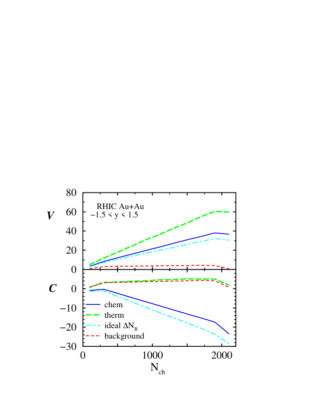
FIG. 1.: Proton variance (top) and proton-antiproton covariance (bottom) for a chemical equilibrium state in RHIC Au+Au. The signature of baryon-density fluctuations – the negative correlation – remains striking in the covariance, despite competition from thermal, volume, and impact-parameter fluctuations.

Having found that chemical equilibrium for baryons can have observable consequences, we now ask whether these particles approach chemical equilibrium in the first place. To be concrete, we suppose that baryons, antibaryons and other hadrons form at a proper time $\tau_{0}$ from the hadronization of a quark gluon plasma. These baryons can then scatter and annihilate, while reactions such as $\rho\omega\rightarrow N\overline{N}$ produce new baryons. Chemical equilibrium is obtained when the annihilation rate precisely matches the creation rate.

To describe the approach to equilibrium, we extend the kinetic model of [9] to include meson-meson production in the following schematic fashion. We take the antibaryon and baryon density to satisfy the approximate kinetic equation:

$$\left({{d}\over{d\tau}}+{{1}\over\tau}\right)n=-\langle\sigma_{a}v_{\rm rel}\rangle\left(n{\overline{n}}-n_{\rm eq}{\overline{n}}_{\rm eq}\right)$$ (19)

together with baryon number conservation. Again we assume a Bjorken-like expansion. Detailed balance for $N\overline{N}\rightleftharpoons$ mesons fixes the product of the chemical equilibrium densities $n_{\rm eq}{\overline{n}}_{\rm eq}$ in terms of the meson densities. Note that this relaxation-time approximation strictly holds only when the initial baryon, antibaryon and meson densities are sufficiently close to local chemical equilibrium values.

In terms of the rapidity densities ${\overline{N}}$ and $N$, we write [9]:

$$\tau{{dN}/{d\tau}}\approx-\gamma~{}\{N{\overline{N}}-N_{\rm eq}{\overline{N}}_{\rm eq}\}.$$ (20)

Baryon conservation implies $N-\overline{N}=N_{B}$. The coefficient $\gamma=\langle\sigma_{a}v_{\rm rel}\rangle{\cal A}^{-1}$ depends on the collision frequency. In [9], we used the measured energy-dependent annihilation cross section to compute $\langle\sigma_{a}v_{\rm rel}\rangle\approx$ 4.4 fm². We take $\overline{N}_{\rm eq}$ to be a $\tau$-independent parameter to be varied over a range of plausible values. This assumption is reasonable for $N$, $\overline{N}\ll N_{\rm tot}$, since the change in the meson populations due to baryon annihilation is then negligible.

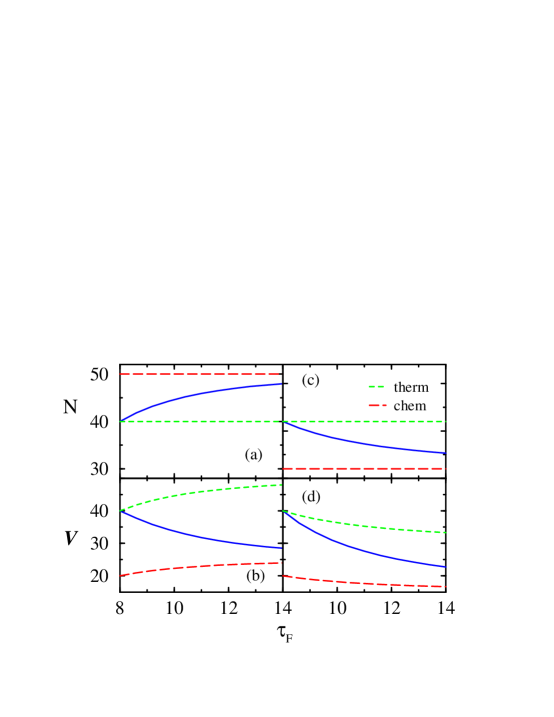
FIG. 2.: The rapid approach to chemical equilibrium of the proton rapidity density (top) and variance (bottom) as functions of the freezeout time $\tau_{F}$ for $N_{\rm eq}>N_{0}$, (a) and (b), and for $N_{\rm eq}<N_{0}$. Hadron formation occurs at $\tau_{0}=8$ fm.

To solve (20), observe that $N(\tau)$ will increase toward $N_{\rm eq}$ depending on whether the right hand side of (20) is positive or negative. Growing solutions are obtained if the initial rapidity density $N_{0}$ satisfies $N_{0}<N_{\rm eq}$, i.e., if the ratio

$$\theta={{N_{\rm eq}-N_{0}}\over{N_{\rm eq}+N_{0}-N_{B}}}$$ (21)

is greater than zero. The solution is then:

$$N={{N_{B}}\over{2}}+\left(N_{\rm eq}-{{N_{B}}\over{2}}\right){{1-\theta S}\over{1+\theta S}}$$ (22)

where

$$S=(\tau_{0}/\tau_{F})^{\gamma(2N_{\rm eq}-N_{B})},$$ (23)

with chemical freezeout occurring at $\tau_{F}$. If $\theta\ll 1$ then annihilation reduces the antiproton-to-proton ratio as in [9]. The evolution of $N$ toward chemical equilibrium is shown in figs. 2a and 2c for $N_{\rm eq}>N_{0}$ and $N_{\rm eq}<N_{0}$, respectively.

To estimate fluctuations in the nonequilbrium state, we write the following ansatz:

$${\cal V}=S{\cal V}_{\rm th}+(1-S){\cal V}_{\rm ch},$$ (24)

where ${\cal V}_{\rm th}$ and ${\cal V}_{\rm ch}$ respectively satisfy (9) and (16). To motivate this ansatz, we consider the variance as a function of $\tau$ and linearize for $N$ near $N_{\rm ch}$, as is standard [10]. We find ${\cal V}\sim{\cal V}_{\rm ch}+2N_{\rm eq}(N(\tau)-N_{\rm eq})$. Differentiating and using (20), we see that $\tau d{\cal V}/d\tau\approx 2\kappa{\cal V}$, where $\kappa\sim d(\log N)/d(\log\tau)\sim-\gamma$. The ansatz (24) has the correct long- and short-scale time dependence to linear order, satisfies the appropriate boundary conditions for $\tau$ near zero and infinity and has plausible behavior for intermediate $\tau$. The ansatz

$${\cal C}=S{\cal C}_{\rm th}+(1-S){\cal C}_{\rm ch},$$ (25)

is similarly plausible.

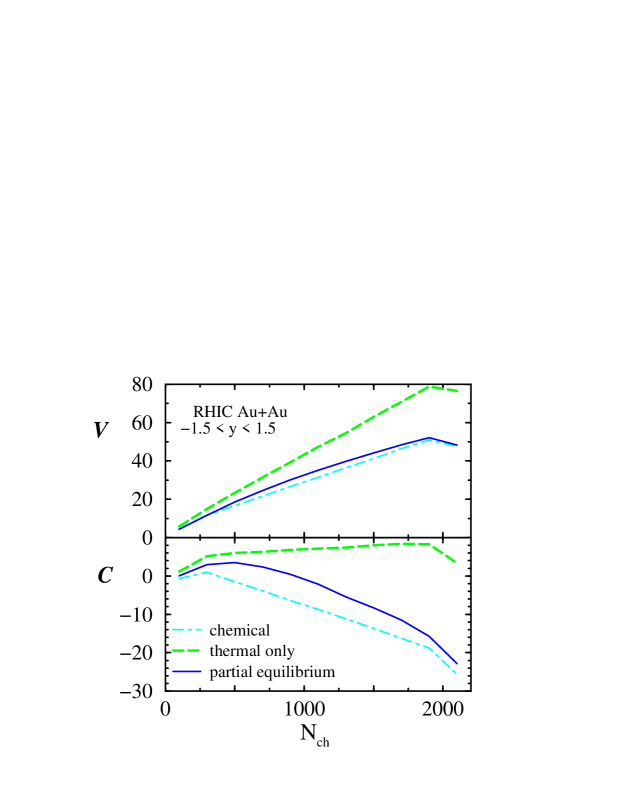
FIG. 3.: Proton variance (top) and covariance (bottom) for a partial chemical equilibrium state in RHIC Au+Au compared to complete chemical (dot-dashed) and thermal equilibrium (long dashed) expectations for the same $N$ and $\overline{N}$.

To appreciate the speed with which equilibration takes place, we show the calculated approach to chemical equilibrium of $N$ and $\cal V$ in fig. 2. We assume that hadronization proceeds from a thermalized quark gluon plasma and, correspondingly, take $\tau_{0}=8$ fm. The initial values $N_{0}\approx\overline{N}_{0}$ are taken from (18) for $b=0$. The chemical freezeout time is varied up to a value $\tau_{F}\approx 14$ fm, a plausible value for central Au+Au at RHIC. For this figure we take ad hoc values for $N_{\rm eq}\approx\overline{N}_{\rm eq}$ to illustrate the approach to equilibrium from above and below. Equilibration is rapid because the annihilation cross section and baryon rapidity densities are sufficiently large that the ratio of the collision time to the expansion time scale satisfies $\tau_{\rm coll}/\tau_{\rm exp}\sim(2\gamma N_{\rm eq})^{-1}<1$.

The variance and covariance computed for the STAR acceptance using $10^{6}$ events simulated according to our partial equilibrium solution are shown in fig. 3. Rapidity densities are computed using (21 - 23) for initial rapidity densities from (18). In these calculations, we take the ad hoc value $N_{\rm eq}=50$ for central collisions and assume $N_{\rm eq}$ scales with the number of participants. The chemical freezeout time is computed for each impact parameter using $\tau_{F}=R/v_{s}+\tau_{p}$, where $R=({\cal A}/\pi)^{1/2}$ is the geometric transverse radius, $v_{s}=1/\sqrt{3}$ is the sound speed and $\tau_{p}\approx 1$ fm is a limiting value for peripheral collisions set by the proton size. Using these values, fluctuations are simulated in accord with (24, 25). We again take the formation time for hadrons to be $\tau_{0}=8$ fm independent of $b$. Note that for values $\tau_{0}\sim 5$ fm or smaller, chemical equilibration is practically complete for impact parameters smaller than 10 fm.

We now ask if such fluctuations can survive freezeout. If chemical freezeout occurs before thermal freezeout, then baryons can suffer elastic collisions with other hadrons after chemical fluctuations are no longer possible. Such scattering can restore $\cal C$ and $\cal V$ to thermal equilibrium values. To estimate the size of this effect, we assume that those baryons and antibaryons that do not scatter elastically contribute to fluctuations at the level of ${\cal V}_{\rm ch}$ and ${\cal C}_{\rm ch}$, while baryons that scatter once or more are instantly thermalized. We then write [12],

$${\cal V}\sim{\cal P}{\cal V}_{\rm ch}+(1-{\cal P}){\cal V}_{\rm th}$$ (26)

where the survival probability for elastic scattering is

$${\cal P}\sim{\rm e}^{-\int_{\tau_{F}}^{\infty}dt\;\sigma v_{\rm rel}n_{\rm tot}(\vec{r}+\vec{v}t,t)},$$ (27)

for $n_{\rm tot}$ the hadron density, $\sigma$ the elastic scattering cross section and $v_{\rm rel}$ the relative velocity. Pions dominate the late-time dynamics, so that $\sigma\approx\sigma_{\pi N}\approx 20$ mb. To estimate $\cal P$, we assume that after chemical freezeout the meson and baryon distributions are described by spherically symmetric Gaussian profiles for both position and velocity. Averaging over these distributions, we find $0.8<{\cal P}<0.9$ for central collisions, assuming $n_{\rm tot}(\tau_{F})\approx 0.1$ fm^-3 and $1<v_{s}\tau_{F}/R<2$.

These calculations suggest that scattering after chemical freezeout increases the chemical equilibrium variances and covariance by less than $20\%$. Scattering at that level is not likely to wipe out the large chemical fluctuations in figs. 1 and 3. Furthermore, UrQMD calculations suggest that chemical freezeout for baryons at RHIC may occur much later than we have assumed [11]. In that case, we expect rescattering to be completely negligible.

In summary, we have found that baryon density fluctuations lead to striking correlations of protons and antiprotons if RHIC collisions approach chemical equilibrium. Measurements of the variance and covariance of these species can reveal these correlations, even if equilibration is incomplete and chemical freezeout precedes thermal freezeout. We have not examined how the $\overline{p}$ and $p$ measurements are altered by resonance decays or hyperon contributions (see [13] for a discussion of resonances in another context). In addition, we have neglected mean field and coulomb effects, which modify correlations over times $\gg\tau_{F}$. Such effects are important when the momentum dependence of correlations is resolved in an HBT-like analysis, see e.g. [14] and refs. therein. Our effect contributes pre-freezeout correlations, often neglected in HBT discussions.

We are grateful to R. Bellwied, P. Fachini, A. Makhlin, R. Venugopalan and N. Xu for discussions. S.G. thanks the nuclear theory group at Brookhaven National Laboratory for hospitality during part of this work. This work is supported in part by the U.S. DOE grant DE-FG02-92ER40713.

REFERENCES

- [1] S. Mrowczynski, Phys. Lett. 72, B430,9 (1998); B439, 6 (1998).
- [2] M. Stephanov, K. Rajagopal and E. Shuryak, Phys Rev Lett 81, 4816 (1998); hep-ph/9903292.
- [3] G. Baym and H. Heiselberg, nucl-th/9905022.
- [4] S. Gavin and C. Pruneau, nucl-th/9906060.
- [5] S. Vance, M. Gyulassy and X.-N. Wang, Phys. Lett. B443, 45 (1998), nucl-th/9806008.
- [6] OPAL Collab., P.D. Acton et al, Phys. Lett. B291, 503 (1992); B305, 415 (1993); TASSO Collab., M. Althoff et al., Z. Phys.C15, 5 (1983).
- [7] T. Sjöstrand, Int. J. Mod. Phys. A3, 751 (1988).
- [8] E. M. Lifshitz and L. O. Pitaevskiii, Statistical Physics Part 1 (Pergamon, 1980), sec. 115.
- [9] S. Gavin, M. Gyulassy, M. Plümer and Venugopalan, Phys. Lett. 234B, 175 (1990).
- [10] E. M. Lifshitz and L. O. Pitaevskiii, Physical Kinetics, (Pergamon, 1981), sec. 19.
- [11] S. A. Bass et al., nucl-th/9902062.
- [12] V. K. Magas et al., nucl-th/9903045.
- [13] S. Jeon and V. Koch, nucl-th/9906074.
- [14] F. Wang and S. Pratt, nucl-th/9908019.