On Tamm’s problem in the Vavilov-Cherenkov radiation theory

Abstract

We analyse the well-known Tamm problem treating the charge motion on a finite space interval with the velocity exceeding light velocity in medium. By comparing Tamm’s formulae with the exact ones we prove that former do not properly describe Cherenkov radiation terms. We also investigate Tamm’s formula $\cos\theta=1/\beta n$ defining the position of maximum of the field strengths Fourier components for the infinite uniform motion of a charge. Numerical analysis of the Fourier components of field strengths shows that they have a pronounced maximum at $\cos\theta=1/\beta n$ only for the charge motion on the infinitely small interval. As the latter grows, many maxima appear. For the charge motion on an infinite interval there is infinite number of maxima of the same amplitude. The quantum analysis of Tamm’s formula leads to the same results.

1 Introduction

In 1888 O. Heaviside considered an infinite charge motion in the nondispersive dielectric infinite medium [1]. He showed that a specific radiation arises when the charge velocity $v$ exceeds the light velocity in medium $c_{n}$. This radiation is confined to the cone with a vertex angle $\sin\theta_{s}=1/\beta_{n}$. Here $\beta_{n}=v/c_{n}$. The Poynting vector being perpendicular to this cone has the angle

$$\cos\theta_{c}=1/\beta_{n}$$

with the motion axis. This radiation was experimentally observed by P.A. Cherenkov in 1934 [2]. Unfortunately, Heaviside’s studies had been forgotten until 1974 when they were revived by A.A. Tyapkin [3] and T.R. Kaiser [4].

I.E. Tamm and I.M. Frank [5] without knowing the previous Heaviside investigations explained Cherenkov’s experiments solving the Maxwell equations in the Fourier representation and subsequently returning to the usual space-time representation. The use of the Fourier representation permitted them to treat the dispersive media as well. For the non-dispersive media they confirmed the validity of Eq.(1.1) defining the direction of the Cherenkov radiation.

In 1939 I.E.Tamm [6] considered the uniform motion of a point charge on the finite space interval with the velocity $v$ exceeding the light velocity in medium $c_{n}$. Here $c_{n}=c/n(\omega)$, $n(\omega)$ is the frequency-dependent refraction index of the medium. He showed that Fourier components of electromagnetic field strengths have a sharp maximum at the angle

$$\cos\theta_{T}=1/\beta_{n}$$

with the motion axis. Here $\beta_{n}=v/c_{n}(\omega)$. Later (see, e.g., [7]) Eq.(1.2) has been extended to the charge motion in an infinite medium.

On the other hand, in Ref. [8] the uniform motion of a point charge was considered in an infinite dispersive medium with a one-pole electric penetrability chosen in a standard way [9]:

$$\epsilon(\omega)=1+\frac{\omega_{L}^{2}}{\omega_{0}^{2}-\omega^{2}}.$$

This expression is a suitable extrapolation between the static case $\epsilon(0)=1+\omega_{L}^{2}/\omega_{0}^{2}$ and the high-frequency limit $\epsilon(\infty)=1$. The electromagnetic potentials, field strengths and the energy flux were evaluated on the surface of a cylinder co-axial with the charge axis motion $z$. They had the main maximum at those points of the cylinder surface where in the absence of dispersion it is intersected by the Cherenkov singular cone and smaller maxima in the interior of this cone. On the other hand, the Fourier transforms of these quantities were oscillating functions of $z$ and, therefore, of the scattering angle $\theta$ ($z=r\cos\theta$) without a pronounced maximum at $\cos\theta=1/\beta_{n}$. This disagrees with the validity of Eq.(1.2) (not (1.1)) for the infinite charge motion.

Lawson [10,11] qualitatively analyzing Tamm’s formula concluded that the distinction between the Cherenkov radiation and bremsstrahlung completely disappears for the small motion interval and is maximal for the large one.

Further, Zrelov and Ruzicka ([12,13]) numerically investigating Tamm’s problem came to the paradoxical result that Tamm’s formulae (which, as they believed, describe the Cherenkov radiation) can be interpreted as the interference of two bremsstrahlung ($BS$) waves emitted at the beginning and end of motion.

Slightly later, the exact solution of the same problem in the absence of dispersion has been found in [14]. It was shown there that Cherenkov’s radiation exists for any motion interval and by no means can be reduced to the interference of two $BS$ waves. This is also confirmed by the results of Ref. [15] where the exact electromagnetic field of a point charge moving with a constant acceleration in medium has been found (the motion begins either from the state of rest or terminates with it).

These inconsistencies and the fact that formula (1.2) for the Fourier components is widely used for the identification of the Cherenkov radiation even for the uniform charge motion in an infinite medium enable us to reexamine Tamm’s problem anew.

The plan of our exposition is as follows. In Sect. 2, we reproduce step by step the derivation of Tamm’s formulae. In Sect. 3, by comparing them with exact ones we prove that Tamm’s approximate formulae do not describe Cherenkov’s radiation properly. The reason for this is due to the approximations involved in their derivation. In Sect. 4, we analyze the validity of Tamm’s formula (1.2) for different intervals of charge motion. We conclude that it is certainly valid for small intervals and breaks for larger ones. This is also supported by the numerical calculations and analytical formula available for the infinite charge motion. On the other hand, the Tamm-Frank formula (1.1) is valid even for the dispersive media: it approximately defines the position of main intensity maximum in the usual space-time representation ([8]). Quantum analysis of Tamm’s formula given in Sect. 5 definitely supports the results of previous sections. A short discussion of the results obtained is given in section 6.

Some precaution is needed. When experimentally investigating a charge motion on a finite interval [16], one usually considers an electron beam entering a thin transparent slab from vacuum, its propagation inside the slab and the subsequent passing into the vacuum on the other side of the slab. The so-called transition radiation [17] arises on the slab interfaces. In this investigation we deal with a pure Tamm’s problem: electron starts at a given point in medium, propagates with a given velocity and then stops at a second point. This may be realized, e.g., for the electron propagation in water where the distance between successive scatters is $\approx 1\mu m$, which is approximately twice the wavelength of the visible Cherenkov radiation [18]. Another realization of Tamm’ problem is a $\beta$ decay followed by the nuclear capture [7,13].

2 Tamm’s problem

Tamm considered the following problem. The point charge rests at the point $z=-z_{0}$ of the $z$ axis up to a moment $t=-t_{0}$. In the time interval $-t_{0}<t<t_{0}$ it uniformly moves along the $z$ axis with the velocity $v$ greater than the light velocity in medium $c_{n}$. For $t>t_{0}$ the charge again rests at the point $z=z_{0}$. The non-vanishing $z$ Fourier component of the vector potential (VP) is given by

$$A_{\omega}=\frac{1}{c}\int_{-z_{0}}^{z_{0}}\frac{1}{R}j_{\omega}(x^{\prime},y^{\prime},z^{\prime})\exp{(-i\omega R/c)}dx^{\prime}dy^{\prime}dz^{\prime},$$

where $R=[(x-x^{\prime})^{2}+(y-y^{\prime})^{2}+(z-z^{\prime})^{2}]^{1/2}$, $j_{\omega}=0$ for $z^{\prime}<-z_{0}$ and $z^{\prime}>z_{0}$ and $j_{\omega}=e\delta(x^{\prime})\delta(y^{\prime})\exp{(-i\omega z^{\prime}/v)}/2\pi$ for $-z_{0}<z^{\prime}<z_{0}$. Inserting all this into $A_{\omega}$ and integrating over $x^{\prime}$ and $y^{\prime}$ one gets

$$A_{\omega}(x,y,z)=\frac{e}{2\pi c}\int_{-z_{0}}^{z_{0}}\frac{dz^{\prime}}{R}\exp{[-i\omega(\frac{z^{\prime}}{v}+\frac{R}{c_{n}})]},$$

$$R=[\rho^{2}+(z-z^{\prime})^{2}]^{1/2},\quad\rho^{2}=x^{2}+y^{2}.$$

At large distances from the charge ($R>>z_{0}$) one has: $R=R_{0}-z^{\prime}\cos\theta,\;\cos\theta=z/R_{0}$. Inserting this into (2.1) and integrating over $z^{\prime}$ one gets

$$A_{\omega}(\rho,z)=\frac{e\beta q(\omega)}{\pi R_{0}\omega}\exp{(-i\omega R_{0}/c_{n})},\quad q(\omega)=\frac{\sin{[\omega t_{0}(1-\beta_{n}\cos\theta)]}}{1-\beta_{n}\cos\theta}.$$

Now we evaluate the field strengths. In the wave zone where $R_{0}>>c/n\omega$ one obtains

$$H_{\phi}=-\frac{2e\beta}{\pi cR_{0}}\sin\theta\int_{0}^{\infty}nq(\omega)\sin[\omega(t-R_{0}/c_{n})]d\omega,$$

$$E_{\rho}=-\frac{2e\beta}{\pi cR_{0}}\sin\theta\cos\theta\int_{0}^{\infty}q(\omega)\sin[\omega(t-R_{0}/c_{n})]d\omega,$$

$$E_{z}=\frac{2e\beta}{\pi cR_{0}}\sin^{2}\theta\int_{0}^{\infty}q(\omega)\sin[\omega(t-R_{0}/c_{n})]d\omega.$$

It should be noted that only the $\theta$ spherical component of $\vec{E}$ differs from zero

$$E_{r}=0,\quad E_{\theta}=-\frac{2e\beta}{\pi cR_{0}}\sin\theta\int_{0}^{\infty}q(\omega)\sin[\omega(t-R_{0}/c_{n})]d\omega.$$

Consider now the function $q(\omega)$. For $\omega t_{0}>>1$ it goes into $\pi\delta(1-\beta_{n}\cos\theta)$. This means that under these conditions $\vec{E}_{\omega}$ and $\vec{H}_{\omega}$ have a sharp maximum for $1-\beta_{n}\cos\theta=0$. Or, in other words, photons with the energy $\hbar\omega$ should be observed at the angle $\cos\theta=1/\beta_{n}$.

The energy flux through the sphere of the radius $R_{0}$ is

$$W=R_{0}^{2}\int S_{r}d\omega,\quad S_{r}=\frac{c}{4\pi}E_{\theta}H\phi.$$

Inserting $E_{\theta}$ and $H_{\phi}$ one obtains

$$W=\frac{2e^{2}\beta^{2}}{\pi c}\int_{0}^{\infty}nJ(\omega)d\omega,\quad J(\omega)=\int_{0}^{\infty}q^{2}\sin\theta d\theta.$$

For $\omega t_{0}>>1$, $J$ can be evaluated in a closed form

$$J=J_{BS}=\frac{1}{\beta^{2}n^{2}}(\ln\frac{1+\beta_{n}}{|1-\beta_{n}|}-2\beta_{n})\quad{\rm for}\quad\beta_{n}<1\quad{\rm and}$$

$$J=J_{BS}+J_{Ch},\quad J_{Ch}=\frac{\pi\omega t_{0}}{\beta_{n}}(1-\frac{1}{\beta_{n}^{2}})\quad{\rm for}\quad\beta_{n}>1.$$

Tamm identified $J_{BS}$ with the spectral distribution of the bremsstrahlung $BS$ , arising from instant acceleration and deceleration of the charge at the moments $\pm t_{0}$, resp. On the other hand, $J_{Ch}$ was identified with the spectral distribution of the Cherenkov radiation. This is supported by the fact that

$$W_{Ch}=\frac{2e^{2}\beta^{2}}{\pi c}\int_{0}^{\infty}nJ_{Ch}(\omega)d\omega=\frac{2e^{2}\beta^{2}t_{0}}{c}\int_{\beta_{n}>1}\omega d\omega(1-\frac{1}{\beta_{n}^{2}}).$$

strongly resembles the famous Frank-Tamm formula [5] for an infinite medium obtained in a quite different way.

In the absence of dispersion Eqs.(2.3) are easily integrated:

$$H_{\phi}^{T}=-\frac{e\beta\sin\theta}{R_{0}(1-\beta_{n}\cos\theta)}\{\delta[c_{n}(t-t_{0})-R_{0}+z_{0}\cos\theta]-\delta[c_{n}(t+t_{0})-R_{0}-z_{0}\cos\theta]\},$$

$$E_{\theta}^{T}=-\frac{e\beta\sin\theta}{R_{0}n(1-\beta_{n}\cos\theta)}\{\delta[c_{n}(t-t_{0})-R_{0}+z_{0}\cos\theta]-\delta[c_{n}(t+t_{0})-R_{0}-z_{0}\cos\theta]\}$$

Superscript $T$ means that these expressions originate from Tamm’s field strengths (2.2).

3 Comparison with exact solution

3.1 Exact solution

On the other hand, in Ref. [14] there was given an exact solution of the treated problem (i.e., the superluminal charge motion on the finite space interval) in the absence of dispersion. It is assumed that a point charge moves on the interval $(-z_{0},z_{0})$ lying inside $S_{0}$. The charge motion begins at the moment $t=-t_{0}=-z_{0}/v$ and terminates at the moment $t=t_{0}=z_{0}/v$. For convenience we shall refer to the $BS$ shock waves emitted at the beginning of the charge motion ($t=-t_{0}$) and at its termination ($t=t_{0}$) as to the $BS_{1}$ and $BS_{2}$ shock waves, resp.

In the wave zone the field strengths are of the form ([14])

$$\vec{E}=\vec{E}_{BS}+\vec{E}_{Ch},\quad\vec{E}_{BS}=\vec{E}_{BS}^{(1)}+\vec{E}_{BS}^{(2)}\quad\vec{H}=\vec{H}_{BS}+\vec{H}_{Ch},$$

$$\vec{H}=H_{\phi}\vec{n}_{\phi},\quad H_{\phi}=H_{BS}+H_{Ch},\quad H_{BS}=H_{BS}^{(1)}+H_{BS}^{(2)}.$$

Here

$$\vec{E}_{BS}^{(1)}=-\frac{e\beta}{n}\frac{\delta[c_{n}(t+t_{0})-r_{1}]}{\beta_{n}(z+z_{0})-r_{1}}\frac{r\sin\theta}{r_{1}}\vec{n}_{\theta}^{(1)},\quad\vec{E}_{BS}^{(2)}=\frac{e\beta}{n}\frac{\delta[c_{n}(t-t_{0})-r_{2}]}{\beta_{n}(z-z_{0})-r_{2}}\frac{r\sin\theta}{r_{2}}\vec{n}_{\theta}^{(2)},$$

$$\vec{E}_{Ch}=\frac{2}{\epsilon r_{m}\gamma_{n}}\delta(c_{n}t-R_{m})\Theta(\rho\gamma_{n}+z_{0}-z)\Theta(-\rho\gamma_{n}+z_{0}+z)\vec{n}_{m},$$

$$H_{BS}^{(1)}=-e\beta\frac{\delta[c_{n}(t+t_{0})-r_{1}]}{\beta_{n}(z+z_{0})-r_{1}}\frac{r\sin\theta}{r_{1}},\quad H_{BS}^{(2)}=e\beta\frac{\delta[c_{n}(t-t_{0})-r_{2}]}{\beta_{n}(z-z_{0})-r_{2}}\frac{r\sin\theta}{r_{2}},$$

$$H_{Ch}=\frac{2}{r_{m}\gamma_{n}\sqrt{\epsilon\mu}}\delta(c_{n}t-R_{m})\Theta(\rho\gamma_{n}+z_{0}-z)\Theta(-\rho\gamma_{n}+z_{0}+z)\vec{n}_{\phi},$$

$$\gamma_{n}=|1-\beta_{n}^{2}|^{-1/2},\quad r_{1}=[(z+z_{0})^{2}+\rho^{2}]^{1/2},\quad r_{2}=[(z-z_{0})^{2}+\rho^{2}]^{1/2},$$

$$r_{m}=[(z-vt)^{2}-\rho^{2}/\gamma_{n}^{2}]^{1/2},\quad R_{m}=(z+\rho/\gamma_{n})/\beta_{n},$$

$$n_{\theta}^{(1)}=[\vec{n}_{\rho}(z+z_{0})-\rho\vec{n}_{z}]/r_{1},\quad n_{\theta}^{(2)}=[\vec{n}_{\rho}(z-z_{0})-\rho\vec{n}_{z}]/r_{2},\quad\vec{n}_{m}=(\vec{n}_{\rho}-n_{z}/\gamma_{n})/\beta_{n}.$$

The meaning of this notation is as follows: $\Theta(x)$ is a step function ($\Theta(x)=0$ for $x<0$ and $\Theta(x)=1$ for $x>0$; $r=\sqrt{z^{2}+\rho^{2}}$ is the distance of the observation point from the origin (it coincides with Tamm’s $R_{0}$); $r_{1}=\sqrt{(z+z_{0})^{2}+\rho^{2}}$ and $r_{2}=\sqrt{(z-z_{0})^{2}+\rho^{2}}$ are the distances of the observation point from the points of the motion axis where the instant acceleration (at $t=-t_{0}$) and deceleration (at $t=t_{0}$) take place. Correspondingly, $\delta$ functions $\delta[c_{n}(t+t_{0})-r_{1}]$ and $\delta[c_{n}(t-t_{0})-r_{2}]$ describe spherical $BS$ shock waves emitted at these moments; $n_{\theta}^{(1)}$ and $n_{\theta}^{(1)}$ are the unit vectors tangent to the above spherical waves and lying in the $\phi=const$ plane; $\vec{E}_{BS}^{(1)}$, $\vec{E}_{BS}^{(2)}$, $\vec{H}_{BS}^{(1)}$ and $\vec{H}_{BS}^{(2)}$ are the electric and magnetic field strengths of the BS shock waves. The function $\delta(c_{n}t-R_{m})$ describes the position of the Cherenkov shock wave ($CSW$). The inequalities $R_{m}<c_{n}t$ and $R_{m}>c_{n}t$ correspond to the points lying inside the VC cone and outside it, resp.; $\vec{n}_{m}$ is the vector lying on the surface of the Vavilov-Cherenkov (VC) cone; $r_{m}$ is the so-called Cherenkov singularity: $r_{m}=0$ on the VC cone surface; $\vec{E}_{Ch}$ and $\vec{H}_{Ch}$ are the electric and magnetic field strengths describing $CSW$; $\vec{E}_{Ch}$ and $\vec{H}_{Ch}$ are infinite on the surface of the VC cone and vanish outside it. Inside the VC cone $\vec{E}_{Ch}$ and $\vec{H}_{Ch}$ decrease as $r^{-2}$ at large distances and, therefore, do not give contribution in the wave zone where only the radiation terms are essential.

3.2 Comparison with Tamm’s solution

At large distances one may develop $r_{1}$ and $r_{2}$ in (3.1): $r_{1}=r+z_{0}\cos\theta,\quad r_{2}=r-z_{0}\cos\theta$. Here $r=R_{0}=[\rho^{2}+z^{2}]^{1/2}$. Neglecting $z_{0}$ compared with $r$ in the denominators of $\vec{E}_{BS}$ and $\vec{H}_{BS}$ in (3.1), one gets

$$\vec{E}_{T}=\vec{E}_{BS},\quad\vec{H}_{T}=\vec{H}_{BS},\quad\vec{E}=\vec{E}_{T}+\vec{E}_{Ch},\quad\vec{H}=\vec{H}_{T}+\vec{H}_{Ch},$$

where $\vec{E}_{T}$ and $\vec{H}_{T}$ are the same as in Eq.(2.6). This means that Tamm’s field strengths (2.6) describe only the bremsstrahlung and do not contain the Cherenkov singular terms. Correspondingly, the maxima of their Fourier transforms refer to the BS radiation.
To elucidate why the Cherenkov radiation is absent in Eqs. (2.3), we consider the product of two $\Theta$ functions entering into the definition (3.1) of Cherenkov field strengths $\vec{E}_{Ch}$ and $\vec{H}_{Ch}$:

$$\Theta(\rho\gamma_{n}+z_{0}-z)\Theta(-\rho\gamma_{n}+z_{0}+z).$$

If for

$$z_{0}<<\rho\gamma_{n}-z=r(\gamma_{n}\sin\theta-\cos\theta)$$

one naively neglects the term $z_{0}$ inside the $\Theta$ functions, the product of two $\Theta$ functions reduces to $\Theta(\rho\gamma_{n}-z)\Theta(-\rho\gamma_{n}+z)$ that is equal to zero. In this case the Cherenkov radiation drops out.

We prove now that essentially the same approximation was implicitly made during the transition from (2.1) to (2.2). When changing $R$ under the sign of exponent in (2.1) by $R_{0}-z^{\prime}\cos\theta$ it was implicitly assumed that the quadratic term in the development of $R$ is small as compared to the linear one. Consider this more carefully. We develop $R$ up to the second order:

$$R\approx R_{0}-z^{\prime}\cos\theta+\frac{z^{\prime 2}}{2R}\sin^{2}\theta.$$

Under the sign of exponent in (2.1) the following terms appear

$$\frac{z^{\prime}}{v}+\frac{1}{c_{n}}(R_{0}-z^{\prime}\cos\theta+\frac{z^{\prime 2}}{2R_{0}}\sin^{2}\theta).$$

We collect terms involving $z^{\prime}$

$$\frac{z^{\prime}}{c_{n}}[(\frac{1}{\beta_{n}}-\cos\theta)+\frac{z^{\prime}}{2R_{0}}\sin^{2}\theta].$$

Taking for $z^{\prime}$ its maximal value $z_{0}$, we present the condition for the second term in the development of $R$ to be small in the form

$$z_{0}<<2R_{0}(\frac{1}{\beta_{n}}-\cos\theta)/\sin^{2}\theta$$

It is seen that the right-hand side of this equation and that of Eq.(3.2) vanish for $\cos\theta=1/\beta_{n}$, i.e., at the angle where the Cherenkov radiation exists. This means that the absence of the Cherenkov radiation in Eqs. (2.3) is due to the omission of second-order terms in the development of $R$ under the exponent in (2.1).

3.3 Space distribution of shock waves

Consider space distribution of the electromagnetic field (EMF) at the fixed moment of time. It is convenient to deal with the space distribution of the magnetic vector potential rather than with that of field strengths which are the space-time derivatives of electromagnetic potentials.
The exact electromagnetic potentials are equal to ([14])

$$\Phi=\Phi_{1}+\Phi_{2}+\Phi_{m}.$$

Here

$$\Phi_{1}=\frac{e}{\epsilon r_{1}}\Theta(r_{1}-c_{n}t-\frac{z_{0}}{\beta_{n}}),\quad\Phi_{2}=\frac{e}{\epsilon r_{2}}\Theta(c_{n}t-r_{2}-\frac{z_{0}}{\beta_{n}}),$$

$$\Phi_{m}=\Phi_{m}^{(1)}+\Phi_{m}^{(2)}+\Phi_{m}^{(3)},\quad A_{z}=A_{z}^{(1)}+A_{z}^{(2)}+A_{z}^{(3)},\quad\Phi_{m}^{(i)}=\frac{1}{\epsilon\beta}A_{z}^{(i)}$$

$$A_{z}^{(1)}=\frac{e\beta}{r_{m}}\Theta(\rho\gamma_{n}-z-z_{0})\Theta(\frac{z_{0}}{\beta_{n}}+r_{2}-c_{n}t)\Theta(c_{n}t+\frac{z_{0}}{\beta_{n}}-r_{1}),$$

$$A_{z}^{(2)}=\frac{e\beta}{r_{m}}\Theta(z-z_{0}-\rho\gamma_{n})\Theta(r_{1}-c_{n}t-\frac{z_{0}}{\beta_{n}})\Theta(c_{n}t-\frac{z_{0}}{\beta_{n}}-r_{2}),$$

$$A_{z}^{(3)}=\frac{e\beta}{r_{m}}\Theta(z_{0}+\rho\gamma_{n}-z)\Theta(z+z_{0}-\rho\gamma_{n})\Theta(c_{n}t-R_{m})\cdot$$

$$[\Theta(r_{1}-c_{n}t-\frac{z_{0}}{\beta_{n}})+\Theta(\frac{z_{0}}{\beta_{n}}+r_{2}-c_{n}t)],$$

(for simplicity we have omitted the $\mu$ factor).

Theta functions

$$\Theta(c_{n}t+\frac{z_{0}}{\beta_{n}}-r_{1})\quad{\rm and}\quad\Theta(r_{1}-c_{n}t-\frac{z_{0}}{\beta_{n}})$$

define space regions which, correspondingly, have and have not been reached by the $BS_{1}$ shock wave. Similarly, theta functions

$$\Theta(c_{n}t-\frac{z_{0}}{\beta_{n}}-r_{2})\quad{\rm and}\quad\Theta(r_{2}-c_{n}t+\frac{z_{0}}{\beta_{n}})$$

define space regions which correspondingly have and have not been reached by the $BS_{2}$ shock wave. Finally, theta function

$$\Theta(c_{n}t-R_{m})$$

defines space region that has been reached by the $CSW$.

The potentials $\Phi_{1}$ and $\Phi_{2}$ correspond to the electrostatic fields of the charge resting at $z=-z_{0}$ up to a moment $-t_{0}$ and at $z=z_{0}$ after the moment $t_{0}$ whilst $\Phi_{m}$ and $A_{z}$ describe the field of a moving charge. Schematic representation of the shock waves position at the fixed moment of time is shown in Fig. 1. In the space regions 1 and 2 corresponding to $z<\rho\gamma_{n}-z_{0}$ and $z>\rho\gamma_{n}+z_{0}$, resp., there are observed only $BS$ shock waves. In the space region 1 (where $A_{z}^{(1)}\neq 0,\quad A_{z}^{(2)}=A_{z}^{(3)}=0$), at the fixed observation point the $BS_{1}$ shock wave (defined by $c_{n}t+z_{0}/\beta_{n}=r_{1}$) arrives first and $BS_{2}$ wave (defined by $c_{n}t-z_{0}/\beta_{n}=r_{2}$) later. In the space region 2 (where $A_{z}^{(2)}\neq 0,\quad A_{z}^{(1)}=A_{z}^{(3)}=0$), these waves arrive in the reverse order. In the space region 3 (where $A_{z}^{(3)}\neq 0,\quad A_{z}^{(1)}=A_{z}^{(2)}=0$), defined by $\rho\gamma_{n}-z_{0}<z<\rho\gamma_{n}+z_{0}$, there are $BS_{1}$, $BS_{2}$ and $CSW$ shock waves. The latter is defined by the equation $c_{n}t=R_{m}$. Before the arrival of the $CSW$ (i.e., for $R_{m}>c_{n}t$) there is an electrostatic field of a charge which is at rest at $z=-z_{0}$. After the arrival of the last of the BS shock waves there is an electrostatic field of a charge which is at rest at $z=z_{0}$. The space region, where $\Phi_{m}$ and $A_{z}$ (and, therefore, the field of a moving charge) differ from zero, lies between the $BS_{1}$ and $BS_{2}$ shock waves in the regions 1 and 2 and between $CSW$ and one of the $BS$ shock waves in the region 3 (for details see Ref. [14]). Space region 3 in its turn consists of two subregions $3_{1}$ and $3_{2}$ defined by the equations $\rho\gamma_{n}-z_{0}<z<(\rho^{2}\gamma_{n}^{2}+z_{0}^{2}/\beta_{n}^{2})^{1/2}$ and $(\rho^{2}\gamma_{n}^{2}+z_{0}^{2}/\beta_{n}^{2})^{1/2}<z<\rho\gamma_{n}+z_{0}$, resp. In the region $3_{1}$ at first there arrive $CSW$, then $BS_{1}$ and, finally, $BS_{2}$. In region $3_{2}$ two last waves arrive in the reverse order.
In brief, $A_{z}^{(1)}$ and $A_{z}^{(2)}$ describe the bremsstrahlung in space regions 1 and 2, resp., while $A_{z}^{(3)}$ describe bremsstrahlung and Cherenkov radiation in space region 3. The polarization vectors of bremsstrahlungs are tangential to the spheres $BS_{1}$ and $BS_{2}$ and lie in the $\phi=const$ plane coinciding with the plane of Fig.1. They are directed along the unit vectors $\vec{n}_{\theta}^{(1)}$ and $\vec{n}_{\theta}^{(2)}$, resp. The polarization vector of $CSW$ (directed along $\vec{n}_{m}$) lies on the CSW. It is shown by the solid line in Fig.1 and also lies in the $\phi=const$ plane. The magnetic field having only the $\phi$ nonvanishing component is normal to the plane of figure. The Poynting vectors defining the direction of the energy transfer are normal to $BS_{1}$, $BS_{2}$ and $CSW$, resp.
The Cherenkov radiation in the ($\rho,z$) plane differs from zero inside the beam of the width $2z_{0}\sin\theta_{c}$, where $\theta_{c}$ is the inclination of the beam towards the motion axis ($\cos\theta_{c}=1/\beta_{n}$). When the charge velocity tends to the velocity of light in medium, the width of the above beam as well as the inclination angle tend to zero. That is, in this case the beam propagates in a nearly forward direction. It is essentially that Cherenkov beam exists for any motion interval $z_{0}$.

3.4 Time evolution of the electromagnetic field on the sphere surface

Consider the distribution of VP (in units $e/R_{0}$) on the sphere $S_{0}$ of the radius $R_{0}$ at different moments of time. There is no EMF on $S_{0}$ up to a moment $T_{n}=1-\epsilon_{0}(1+1/\beta_{n})$. Here $T_{n}=c_{n}t/R_{0}$. In the time interval

$$1-\epsilon_{0}(1+\frac{1}{\beta_{n}})\leq T_{n}\leq 1-\epsilon_{0}(1-\frac{1}{\beta_{n}})$$

BS radiation begins to fill the back part of $S_{0}$ corresponding to the angles

$$-1<\cos\theta<\frac{1}{2\epsilon_{0}}[(T_{n}+\frac{\epsilon_{0}}{\beta_{n}})^{2}-1-\epsilon_{0}^{2}]$$

(Fig. 2a, curve 1). In the time interval

$$1-\epsilon_{0}(1-\frac{1}{\beta_{n}})\leq T_{n}\leq[1-(\frac{\epsilon_{0}}{\beta_{n}\gamma_{n}})^{2}]^{1/2}$$

BS radiation begins to fill the front part of $S_{0}$ as well:

$$\frac{1}{2\epsilon_{0}}[1+\epsilon_{0}^{2}-(T_{n}-\frac{\epsilon_{0}}{\beta_{n}})^{2}]\leq\cos\theta\leq 1.$$

The illuminated back part of $S_{0}$ is still given by (3.5) (Fig. 2a, curve 2). The finite jumps of VP shown in these figures lead to the $\delta$-type singularities in Eqs. (3.1) defining BS electromagnetic strengths. In the time intervals (3.4) and (3.6) these jumps have a finite height. The vector potential is maximal at the angle at which the jump occurs. The value of VP is infinite at the angles defined by

$$\cos\theta_{1}=-\frac{\epsilon_{0}}{\beta_{n}^{2}\gamma_{n}^{2}}+\frac{1}{\beta_{n}}[1-(\frac{\epsilon_{0}}{\beta_{n}\gamma_{n}})^{2}]^{1/2}\quad{\rm and}\quad\cos\theta_{2}=\frac{\epsilon_{0}}{\beta_{n}^{2}\gamma_{n}^{2}}+\frac{1}{\beta_{n}}[1-(\frac{\epsilon_{0}}{\beta_{n}\gamma_{n}})^{2}]^{1/2}.$$

which are reached at the time

$$T_{Ch}=\frac{c_{n}t_{Ch}}{R_{0}}=[1-(\frac{\epsilon_{0}}{\beta_{n}\gamma_{n}})^{2}]^{1/2}$$

(Fig. 2a, curve 3). At this moment and at these angles the $CSW$ intersects $S_{0}$ first time. Or, in other words, the intersection of $S_{0}$ by the lines $z=\rho\gamma_{n}-z_{0}$ and $z=\rho\gamma_{n}+z_{0}$ (Fig.1) occurs at the angles $\theta_{1}$ and $\theta_{2}$. At this moment the illuminated front and back parts of $S_{0}$ are given by $\theta_{1}<\theta<\pi$ and $0<\theta<\theta_{2}$, resp. Beginning from this moment, the $CSW$ intersects the sphere $S_{0}$ at the angles defined by (see Fig. 2b)

$$\cos\theta_{Ch}^{(1)}(T)=\frac{T_{n}}{\beta_{n}}-\frac{1}{\beta_{n}\gamma_{n}}(1-T_{n}^{2})^{1/2}\quad{\rm and}\quad\cos\theta_{Ch}^{(2)}(T)=\frac{T_{n}}{\beta_{n}}+\frac{1}{\beta_{n}\gamma_{n}}(1-T_{n}^{2})^{1/2}.$$

The positions of the $BS_{1}$ and $BS_{2}$ shock waves are given by

$$\cos\theta_{BS}^{(1)}(T)=\frac{1}{2\epsilon_{0}}[(T_{n}+\frac{\epsilon_{0}}{\beta_{n}})^{2}-1-\epsilon_{0}^{2}]\quad{\rm and}\quad\cos\theta_{BS}^{(2)}(T)=\frac{1}{2\epsilon_{0}}[1+\epsilon_{0}^{2}-(T_{n}-\frac{\epsilon_{0}}{\beta_{n}})^{2}],$$

respectively (i.e., the $BS$ shock waves follow after the $CSW$). Therefore, at this moment $BS$ fills the angle regions

$$\theta_{BS}^{(1)}(T)\leq\theta\leq\pi\quad{\rm and}\quad 0\leq\theta\leq\theta_{BS}^{(2)}(T)$$

while the VC radiation occupies the angle interval

$$\theta_{Ch}^{(1)}(T)\leq\theta\leq\theta_{1}\quad{\rm and}\quad\theta_{2}\leq\theta\leq\theta_{Ch}^{(2)}(T)$$

Therefore, VC radiation field and $BS$ overlap in the regions

$$\theta_{BS}^{(1)}(T)\leq\theta\leq\theta_{1}\quad{\rm and}\quad\theta_{2}\leq\theta\leq\theta_{BS}^{(2)}(T).$$

$BS_{1}$ and $BS_{2}$ have finite jumps in this angle interval (Fig. 2b). The non-illuminated part of $S_{0}$ is

$$\theta_{Ch}^{(2)}(T)\leq\theta\leq\theta_{Ch}^{(1)}(T).$$

This lasts up to a moment $T_{n}=1$ when the Cherenkov shock wave intersects $S_{0}$ only once at the point corresponding to the angle $\cos\theta=1/\beta_{n}$ (Fig. 2c). The positions of the $BS_{1}$ and $BS_{2}$ shock waves at this moment ($T_{n}=1$) are given by

$$\cos\theta=\frac{1}{\beta_{n}}-\frac{\epsilon_{0}}{2\beta_{n}^{2}\gamma_{n}^{2}}\quad{\rm and}\quad\cos\theta=\frac{1}{\beta_{n}}+\frac{\epsilon_{0}}{2\beta_{n}^{2}\gamma_{n}^{2}},$$

resp. Again, the jumps of BS waves have finite heights while the Cherenkov potentials (and field strengths) are infinite at the angle $\cos\theta=1/\beta_{n}$ where $CSW$ intersects $S_{0}$
After the moment $T_{n}=1$, $CSW$ leaves $S_{0}$. However, the Cherenkov post-action still remains (Fig. 3a). At the subsequent moments of time the $BS_{1}$ and $BS_{2}$ shock waves approach each other. They meet at the moment

$$T_{n}=[1+(\frac{\epsilon_{0}}{\beta_{n}\gamma_{n}})^{2}]^{1/2}.$$

at the angle

$$\cos\theta=\frac{1}{\beta_{n}}[1+(\frac{\epsilon_{0}}{\beta_{n}\gamma_{n}})^{2}]^{1/2}.$$

After this moment BS shock waves pass through each other and diverge (Fig. 3b). Now $BS_{1}$ and $BS_{2}$ move along the front and back semi-spheres, resp. There is no EMF on the part of $S_{0}$ lying between them. The illuminated parts of $S_{0}$ are now given by

$$\theta_{BS}^{(2)}(T)\leq\theta\leq\pi\quad{\rm and}\quad 0\leq\theta\leq\theta_{BS}^{(1)}(T)$$

The electromagnetic field is zero inside the angle interval

$$\theta_{BS}^{(1)}(T)\leq\theta\leq\theta_{BS}^{(2)}(T).$$

After the moment of time (3.8) $BS_{1}$ and $BS_{2}$ may occupy the same angular positions $cos\theta_{2}$ and $cos\theta_{1}$ like $BS_{2}$ and $BS_{1}$ shown by curve 3 in Fig. 2a. But now their jumps are finite. After the moment

$$T_{n}=1+\epsilon_{0}(1-\frac{1}{\beta_{n}})$$

the front part of $S_{0}$ begins not to be illuminated (Fig. 3c). At this moment the illuminated back part of $S_{0}$ is given by

$$-1\leq\cos\theta\leq-1+\frac{2(1+\epsilon_{0})}{\beta_{n}}-\frac{2\epsilon_{0}}{\beta_{n}^{2}}.$$

In the subsequent time the illuminated part of $S_{0}$ is given by

$$-1\leq\cos\theta\leq\frac{1}{2\epsilon_{0}}[1+\epsilon_{0}^{2}-(T_{n}-\frac{\epsilon_{0}}{\beta_{n}})^{2}]$$

. As time goes, the illuminated part of $S_{0}$ diminishes. Finally , after the moment

$$T_{n}=1+\epsilon_{0}(1+\frac{1}{\beta_{n}})$$

the EMF radiation leaves the surface of $S_{0}$ (and its interior).

We summarize here main differences between Cherenkov radiation and bremsstrahlung:
On the sphere $S_{0}$, VC radiation runs over the angular region

$$\theta_{2}\leq\theta\leq\theta_{1},$$

where $\theta_{1}$ and $\theta_{2}$ are defined by Eqs. (3.7). At each particular moment of time $T_{n}$ in the interval

$$[1-(\frac{\epsilon_{0}}{\beta_{n}\gamma_{n}})^{2}]^{1/2}\leq T_{n}\leq 1$$

the VC electromagnetic potentials and field strengths are infinite at the angles $\theta_{Ch}^{(1)}(T)$ and $\theta_{Ch}^{(2)}(T)$ at which $CSW$ intersects $S_{0}$.
After the moment $T_{n}=1$ the Cherenkov singularity leaves the sphere $S_{0}$, but the Cherenkov post-action still remains. This lasts up to the moment $T_{n}=[1+(\epsilon_{0}/\beta_{n}\gamma_{n})^{2}]^{1/2}$.
On the other hand, $BS$ runs over the whole sphere $S_{0}$ in the time interval

$$1-\epsilon_{0}(1+\frac{1}{\beta_{n}})\leq T_{n}\leq 1+\epsilon_{0}(1+\frac{1}{\beta_{n}}).$$

The vector potential of $BS$ is infinite only at the angles $\theta_{1}$ and $\theta_{2}$ at the particular moment of time $T_{n}=\sqrt{1-\epsilon_{0}^{2}/\beta_{n}^{2}\gamma_{n}^{2}}$ when $CSW$ first time intersects $S_{0}$. For other times the VP of $BS$ exhibits finite jumps in the angle interval $-\pi\leq\theta\leq\pi$. The $BS$ electromagnetic field strengths (as space-time derivatives of electromagnetic potentials) are infinite at those angles. Therefore, Cherenkov singularities of the vector potential run over the region $\theta_{2}\leq\theta\leq\theta_{1}$ of the sphere $S_{0}$, while the $BS$ vector potential is infinite only at the angles $\theta_{1}$ and $\theta_{2}$ where $BS$ shock waves meet $CSW$.

The following particular cases are of special interest. For small $\epsilon_{0}=z_{0}/R_{0}$ the Cherenkov singular radiation occupies the narrow angular region

$$\frac{1}{\beta_{n}}-\frac{\epsilon_{0}}{\beta_{n}^{2}\gamma_{n}^{2}}\leq\cos\theta\leq\frac{1}{\beta_{n}}+\frac{\epsilon_{0}}{\beta_{n}^{2}\gamma_{n}^{2}},$$

while BS is infinite at the boundary points of this interval ( at $\cos\theta=\frac{1}{\beta_{n}}\pm\frac{\epsilon_{0}}{\beta_{n}^{2}\gamma_{n}^{2}}$) reached at the moment $T_{n}=1-\epsilon_{0}^{2}/2\beta_{n}^{2}\gamma_{n}^{2}$.
In the opposite case ($\epsilon_{0}\approx 1$) the singular Cherenkov radiation field is confined to the angular region

$$\frac{2}{\beta_{n}^{2}}-1\leq\cos\theta\leq 1,$$

while BS has singularities at $\cos\theta=\frac{2}{\beta_{n}^{2}}-1,\quad{\rm and}\quad\cos\theta=1$ reached at the moment $T_{n}=1/\beta_{n}$.
When the charge velocity is close to the light velocity in medium ($\beta_{n}\approx 1$), one gets:

$$\cos\theta_{1}\approx\frac{1}{\beta_{n}}-\frac{\epsilon_{0}}{\beta_{n}^{2}\gamma_{n}^{2}}(1+\frac{1}{2}\epsilon_{0})\approx 1,\quad\cos\theta_{2}\approx\frac{1}{\beta_{n}}-\frac{\epsilon_{0}}{\beta_{n}^{2}\gamma_{n}^{2}}(1-\frac{1}{2}\epsilon_{0})\approx 1,$$

i.e., there is a narrow Cherenkov beam in the nearly forward direction.

3.5 Comparison with Tamm’s vector potential

Now we evaluate Tamm’s VP

$$A_{T}=\int\limits_{-\infty}^{\infty}d\omega\exp{(i\omega t)}A_{\omega}$$

Substituting here $A_{\omega}$ given by (2.2), we get in the absence of dispersion

$$A_{T}=\frac{e}{R_{0}n|\cos\theta-1/\beta_{n}|}\Theta(|\cos\theta-1/\beta_{n}|-|T_{n}-1|/\epsilon_{0}).$$

This VP may be also obtained from $A_{z}$ given by (3.3) if we leave in it the terms $A_{z}^{(1)}$ and $A_{z}^{(2)}$ describing BS in the regions 1 and 2 (see Fig.1) (with omitting $z_{0}$ in the factors $\Theta(\rho\gamma_{n}-z-z_{0})$ and $\Theta(z-z_{0}-\rho\gamma_{n})$ entering into them) and drop the term $A_{z}^{(3)}$ which is responsible (as we have learned from the previous section) for the $BS$ and $VC$ radiation in region 3 and which describes a very thin Cherenkov beam in the limit $\epsilon_{0}\to 0$. It is seen at once that $A_{z}$ is infinite only at

$$T_{n}=1,\quad\cos\theta=1/\beta_{n}.$$

This may be compared with the exact consideration of the previous section which shows that the $BS$ part of $A_{z}$ is infinite at the moment

$$T_{Ch}=\frac{c_{n}t_{Ch}}{R_{0}}=[1-(\frac{\epsilon_{0}}{\beta_{n}\gamma_{n}})^{2}]^{1/2}$$

at the angles $\cos\theta_{1}$ and $\cos\theta_{2}$ defined by (3.7). It is seen, $\cos\theta_{1}$ and $\cos\theta_{2}$ defined by (3.7) and $T_{Ch}$ given by (3.11) are transformed into $\cos\theta$ and $T_{n}$ given by (3.10) in the limit $\epsilon_{0}\to 0$. Due to the dropping of the $A_{z}^{(3)}$ term in (3.3) (describing bremsstrahlung and Cherenkov radiation in space region 3) and the omission of terms containing $\epsilon_{0}$ in $\cos\theta_{1}$ and $\cos\theta_{2}$, $BS_{1}$ and $BS_{2}$ waves have now the common maximum of the infinite height at the angle $\cos\theta=1/\beta_{n}$ where Tamm’s approximation fails.

The analysis of (3.9) shows that Tamm’s VP is distributed over $S_{0}$ in the following way. There is no EMF of the moving charge up to the moment $T_{n}=1-\epsilon_{0}(1+1/\beta_{n})$. For

$$1-\epsilon_{0}(1+\frac{1}{\beta_{n}})<T_{n}<1-\epsilon_{0}(1-\frac{1}{\beta_{n}})$$

EMF fills only the back part of $S_{0}$

$$-1<\cos\theta<\frac{1}{\beta_{n}}-\frac{1}{\epsilon_{0}}(1-T_{n})$$

(Fig. 4a, curve 1). In the time interval

$$1-\epsilon_{0}(1-\frac{1}{\beta_{n}})<T_{n}<1+\epsilon_{0}(1-\frac{1}{\beta_{n}})$$

the illuminated parts of $S_{0}$ are given by

$$-1<\cos\theta<\frac{1}{\beta_{n}}-\frac{1}{\epsilon_{0}}(1-T_{n})\quad{\rm and}\quad\frac{1}{\beta_{n}}+\frac{1}{\epsilon_{0}}(1-T_{n})<\cos\theta<1$$

(Fig. 4a, curves 2 and 3). The jumps of the $BS_{1}$ and $BS_{2}$ shock waves are finite. As $T_{n}$ tends to 1, the $BS_{1}$ and $BS_{2}$ shock waves approach each other and fuse at $T_{n}=1$. Tamm’ VP is infinite at this moment at the angle $\cos\theta=1/\beta_{n}$ (Fig. 4b). For

$$1<T_{n}<1+\epsilon_{0}(1-\frac{1}{\beta_{n}})$$

the $BS$ shock waves pass through each other and begin to diverge, $BS_{1}$ and $BS_{2}$ filling the front and back parts of $S_{0}$, resp. (Fig. 4c):

$$\frac{1}{\beta_{n}}+\frac{1}{\epsilon_{0}}(T_{n}-1)<\cos\theta<1\quad(BS_{1})\quad{\rm and}$$

$$-1<\cos\theta<\frac{1}{\beta_{n}}-\frac{1}{\epsilon_{0}}(T_{n}-1)\quad(BS_{2}).$$

For larger times

$$1+\epsilon_{0}(1-\frac{1}{\beta_{n}})<T_{n}<1+\epsilon_{0}(1+\frac{1}{\beta_{n}})$$

only back part of $S_{0}$ is illuminated:

$$-1<\cos\theta<\frac{1}{\beta_{n}}-\frac{1}{\epsilon_{0}}(T_{n}-1)\quad(BS_{2}).$$

Finally, for $T_{n}>1+\epsilon_{0}(1+1/\beta_{n})$ there is no radiation field on $S_{0}$ and inside it.
It is seen that the behaviour of exact and approximate Tamm’s potentials is very alike in the space regions 1 and 2 where Cherenkov radiation is absent and differs appreciably in the space region 3 where it exists. Roughly speaking, Tamm’s vector potential (3.9) describing evolution of BS shock waves in the absence of $CSW$ imitates the latter in the neighborhood of $\cos\theta=1/\beta_{n}$ where, as we know from sect. (3.2), Tamm’s approximate VP is not correct.
This complication is absent if the charge velocity $\beta$ is less than light velocity in medium $\beta_{c}$. In this case one the exact VP is (see [14]):

$$A_{z}=\frac{e\beta\mu}{r_{m}}\Theta[c_{n}(t+t_{0})-r_{1}]\Theta[r_{2}-c_{n}(t-t_{0})],$$

while Tamm’s VP $A_{T}$ is still given by (3.9). The results of calculations for $\beta=0.7,\quad\beta_{c}\approx 0.75$ are presented in Fig. 5. We see on it the exact and Tamm’s VPs for three typical times: $T=1.26;\quad T=1.334$ and $T=1.4$. In general, EMF distribution on the sphere surface is as follows. There is no field on $S_{0}$ up to some moment of time. Later, only back part of $S_{0}$ is illuminated (see Fig. 5a). In the subsequent times the EMF fills the whole sphere (Fig. 5 b). After some moment, the EMF again fills only the back part of $S_{0}$ (Fig. 5c). Finally, EMF leaves $S_{0}$.

Now we analyze the behaviour of Tamm’s VP for small and large motion intervals $z_{0}$. For small $\epsilon_{0}=z_{0}/R_{0}$ it follows from (3.9) that $A_{z}=0$ except for the moment $T_{n}=1$ when

$$A_{z}=\frac{e}{R_{0}n|\frac{1}{\beta_{n}}-\cos\theta|}.$$

On the other hand, if we pass to the limit $\epsilon_{0}\to 0$ in Eq.(2.2), i.e., prior to the integration, then

$$A_{\omega}\to\frac{e\epsilon_{0}}{\pi c}\exp(-i\omega R_{0}/c_{n}),\quad A_{z}\to\frac{e\epsilon_{0}}{\pi nR_{0}}\delta(T_{n}-1),$$

i.e., there is no angular dependence in (3.14). The distinction of (3.14) from (3.13) is due to the fact that integration takes place for all $\omega$ in the interval ($-\infty,+\infty$). For large $\omega$ the condition $\omega z_{0}/v<<1$ is violated. This means that Eq. (3.13) is more correct.
For large $z_{0}$ one gets from (3.9)

$$A_{z}=\frac{e}{R_{0}n|\frac{1}{\beta_{n}}-\cos\theta|}.$$

If we take the limit $z_{0}\to\infty$ in Eq.(2.2), then

$$A_{\omega}\approx\frac{e\beta}{R_{0}\omega}\exp(-i\omega R_{0}/c_{n})\delta(1-\beta_{n}\cos\theta)\quad A_{z}(t)\sim\delta(1-\beta_{n}\cos\theta).$$

Although Eqs.(3.15) and (3.16) reproduce the position of Cherenkov singularity at $\cos\theta=1/\beta_{n}$, they do not describe the Cherenkov cone. The reason for this is that Tamm’s VP (2.2) is obtained under the condition $z_{0}<<R_{0}$ and, therefore, it is not legitimate to take the limit $z_{0}\to\infty$ in the expressions following from it (and, in particular, in Eq. (3.9)).
On the other hand, taking the limit $z_{0}\to\infty$ in the exact expression (3.3) we get the well-known expressions for the electromagnetic potentials describing superluminal motion of charge in an infinite medium:

$$A_{z}=\frac{2e\beta\mu}{r_{m}}\Theta(vt-z-\rho/\gamma_{n}),\quad\Phi=\frac{2e}{\epsilon r_{m}}\Theta(vt-z-\rho/\gamma_{n}).$$

The very fact that Tamm’ VP (3.9) is valid both for $\beta<\beta_{c}$ and $\beta>\beta_{c}$ has given rise to the extensive discussion in the physical literature concerning the discrimination between the BS and Cherenkov radiation. From the facts that: i) Eq.(3.13), following from Tamm’s VP (2.2) in the limit of small $z_{0}$, does not contain the angular dependence and ii) this dependence presents in Eq. (3.15) (which differs from zero only for $\beta_{n}>1$) following from the same Eq.(2.2) in the limit of large $z_{0}$ it is frequently stated (see, e.g., [10,11]) that distinction between the Cherenkov radiation and bremsstrahlung disappears for $z_{0}\to 0$ and is maximal for $z_{0}\to\infty$.

As it follows from our consideration, the physical reason for this is due to the absence of Cherenkov radiation in Tamm’s VP (3.9). Exact electomagnetic potentials (3.3) and field strengths (3.1) contain Cherenkov radiation for any $z_{0}$. The induced Cherenkov beam being very thin for $z_{0}\to 0$ and broad for large $z_{0}$, not in any case can be reduced to the bremsstrahlung.

This is also confirmed by the consideration of the semi-infinite accelerated motion of a charged particle in a non-dispersive medium [15]. The arising Cherenkov radiation and bremsstrahlung are clearly separated, no ambiguity arises in their interpretation.

4 Space distribution of Fourier components

The Fourier transform of the vector potential on the sphere $S_{0}$ of the radius $R_{0}$ is given by

$$ReA_{\omega}=\frac{e}{2\pi c}\int\limits_{-\epsilon_{0}}^{\epsilon_{0}}\frac{dz}{Z}\cos[\frac{R_{0}\omega}{c_{n}}(\frac{z}{\beta_{n}}+Z)],$$

$$ImA_{\omega}=-\frac{e}{2\pi c}\int\limits_{-\epsilon_{0}}^{\epsilon_{0}}\frac{dz}{Z}\sin[\frac{R_{0}\omega}{c_{n}}(\frac{z}{\beta_{n}}+Z)]$$

Here $Z=(1+z^{2}-2z\cos\theta)^{1/2}$. For $z_{0}<<R_{0}$ these expressions should be compared with the real and imaginary parts of Tamm’s approximate VP (2.2):

$$ReA_{\omega}=\frac{e\beta q}{\pi R_{0}\omega}\cos(\frac{\omega R_{0}}{c_{n}}),\quad ImA_{\omega}=-\frac{e\beta q}{\pi R_{0}\omega}\sin(\frac{\omega R_{0}}{c_{n}}).$$

These quantities are evaluated (in units $e/2\pi c$) for

$$\frac{\omega R_{0}}{c_{n}}=100,\quad\beta=0.99,\quad n=1.334,\quad\epsilon_{0}=0.1$$

(see Figs. 6 a, b). We observe that angular distributions of VPs (4.1) and (4.2) practically coincide having maxima on the small part of $S_{0}$ in the neighborhood of $\cos\theta=1/\beta_{n}$. It is this minor difference between (4.1) and (4.2) that is responsible for the Cherenkov radiation which is described only by Eq. (4.1).
Now we evaluate the angular dependence of VP (4.1) on the sphere $S_{0}$ for the case when $z_{0}$ practically coincides with $R_{0}$ ($\epsilon_{0}=0.98$). Other parameters remain the same. We see ( Fig. 6c) that angular distribution fills the whole sphere $S_{0}$. There is no pronounced maximum in the vicinity of $\cos\theta=1/\beta_{n}$.
We cannot extend these results to larger $z_{0}$ as the motion interval will partly lie outside $S_{0}$. To consider a charge motion on an arbitrary finite interval, we evaluate the distribution of VP on the cylinder surface $C$ co-axial with the motion axis. Let the radius of this cylinder be $\rho$. Making the change of variables $z=z^{\prime}+\rho\sinh\chi$ under the sign of integral in (2.1), one obtains

$$ReA_{\omega}=\frac{e}{2\pi c}\int\limits_{x_{1}}^{x_{2}}\cos[\frac{\omega\rho}{c}(\frac{z}{\rho\beta}+\frac{1}{\beta}\sinh\chi+n\cosh\chi)]d\chi,$$

$$ImA_{\omega}=-\frac{e}{2\pi c}\int\limits_{x_{1}}^{x_{2}}\sin[\frac{\omega\rho}{c}(\frac{z}{\rho\beta}+\frac{1}{\beta}\sinh\chi+n\cosh\chi)]d\chi,$$

where $x_{1}=arcsinh\chi_{1},\quad x_{2}=arcsinh\chi_{2},\quad\sinh\chi_{1}=-(z_{0}+z)/\rho,\quad\sinh\chi_{2}=(z_{0}-z)/\rho$.
The distributions of $ReA_{\omega}$ and $ImA_{\omega}$ (in units $e/2\pi c$) on the surface of $C$ as function of $\tilde{z}=z/\rho$ are shown in Figs 7,8 for different values of $\epsilon_{0}=z_{0}/\rho$ and $\rho$ fixed. The calculations were made for $\beta=0.99$ and $\omega\rho/c=100$. We observe that for small $\epsilon_{0}$ the electromagnetic field differs from zero only in the vicinity $\tilde{z}=\gamma_{n}$, which corresponds to $\cos\theta=1/\beta_{n}$ (Fig., 7 a and b). As $\epsilon_{0}$ increases, the VP begin to diffuse over the cylinder surface. This is illustrated in Figs. 7,c and 8,a where only the real parts of $A_{\omega}$ for $\epsilon_{0}=1$ and $\epsilon_{0}=10$ are presented. Since the behaviour of $ReA_{\omega}$ and $ImA_{\omega}$ is very much alike (Figs. 6, 7 a and b clearly demonstrate this), we limit ourselves to the consideration of $ReA_{\omega}$). We observe the disappearance of pronounced maxima at $\cos\theta=1/\beta_{n}$. For the infinite motion ($z_{0}\to\infty$) Eqs. (4.3) reduce to

$$ReA_{\omega}=\frac{e}{2\pi c}\int\limits_{-\infty}^{\infty}\cos[\frac{\omega\rho}{c}(\frac{z}{\rho\beta}+\frac{1}{\beta}\sinh\chi+n\cosh\chi)]d\chi,$$

$$ImA_{\omega}=-\frac{e}{2\pi c}\int\limits_{-\infty}^{\infty}\sin[\frac{\omega\rho}{c}(\frac{z}{\rho\beta}+\frac{1}{\beta}\sinh\chi+n\cosh\chi)]d\chi.$$

These expressions can be evaluated in the analytical form (see Appendix)

$$\frac{ReA_{\omega}}{e/2\pi c}=-\pi[J_{0}(\frac{\omega\rho}{v\gamma_{n}})\sin(\frac{\omega z}{v})+N_{0}(\frac{\omega\rho}{v\gamma_{n}})\cos(\frac{\omega z}{v})],$$

$$\frac{ImA_{\omega}}{e/2\pi c}=\pi[N_{0}(\frac{\omega\rho}{v\gamma_{n}})\sin(\frac{\omega z}{v})-J_{0}(\frac{\omega\rho}{v\gamma_{n}})\cos(\frac{\omega z}{v})]$$

for $v>c_{n}$ and

$$\frac{ReA_{\omega}}{e/2\pi c}=2\cos(\frac{\omega z}{v})K_{0}(\frac{\rho\omega}{v\gamma_{n}}),\quad\frac{ImA_{\omega}}{e/2\pi c}=-2\sin(\frac{\omega z}{v})K_{0}(\frac{\rho\omega}{v\gamma_{n}})$$

for $v<c_{n}$ (remember that $\gamma_{n}=|1-\beta_{n}^{2}|^{-1/2}$). We see that for the infinite charge motion the Fourier transform $A_{\omega}$ is a pure periodical function of $z$ (and, therefore, of the angle $\theta$). This assertion does not depend on the $\rho$ and $\omega$ values. For example, for $\omega\rho/v\gamma_{n}>>1$ one gets

$$\frac{ReA_{\omega}}{e/2\pi c}=-\sqrt{\frac{2v\pi\gamma_{n}}{\rho\omega}}\sin[\frac{\omega}{v}(z+\frac{\rho}{\gamma_{n}})-\frac{\pi}{4}],\quad\frac{ImA_{\omega}}{e/2\pi c}=-\sqrt{\frac{2v\pi\gamma_{n}}{\rho\omega}}\cos[\frac{\omega}{v}(z+\frac{\rho}{\gamma_{n}})-\frac{\pi}{4}]$$

for $v>c_{n}$ and

$$\frac{ReA_{\omega}}{e/2\pi c}=\sqrt{\frac{2v\pi\gamma_{n}}{\rho\omega}}\cos(\frac{\omega z}{v})\exp(-\frac{\rho\omega}{v\gamma_{n}}),\quad\frac{ImA_{\omega}}{e/2\pi c}=-\sqrt{\frac{2v\pi\gamma_{n}}{\rho\omega}}\sin(\frac{\omega z}{v})\exp(-\frac{\rho\omega}{v\gamma_{n}})$$

for $v<c_{n}$.

In Fig. 8b, by comparing the real part of $A_{\omega}$ evaluated according to Eq.(4.3) for $\epsilon_{0}=10$ with the analytical expression (4.5) valid for $\epsilon_{0}\to\infty$ we observe their perfect agreement on the small interval of cylinder $C$ surface (they are indistinguishable on the treated interval). The same coincidence is valid for $ImA_{\omega}$.

As it is explicitly stated in [10,11], Tamm’s approximate Fourier component of VP (2.2) has the $\delta$-type singularity at the Cherenkov angle for $z_{0}\to\infty$ (see Eq.(3.16)) and is independent of angle for $z_{0}\to 0$ (Eq.(3.14)). However, the behaviour of the exact Fourier component of VP is exactly opposite to this behaviour: $A(\omega)$ has an isolated maximum for the very small motion intervals and has infinite number of maxima for $z_{0}\to\infty$.

The absence of the isolated pronounced maximum of potentials and field strengths at $\cos\theta=1/\beta_{n}$ for the charge motion on the finite interval may qualitatively be understood as follows. We begin with the exact equations (3.1) and (3.3) for the field strengths and potentials in the space-time representation. Making inverse Fourier transform from them, we arrive at Eqs. (4.1)-(4.5) of this section. Now, if the charge motion takes place on the small space interval, field strengths and potentials (3.1) and (3.3) have singularities on a rather small space-time interval (as the Cherenkov beam is thin in this case). Therefore, Fourier transforms of (3.1) and (3.3) should be different from zero in the limited space region. For the charge motion on a large interval field strengths and potentials (3.1) and (3.3) have singularities in a larger space-time domain (as the Cherenkov beam is a rather broad now). Consequently, Fourier transforms of (3.1) and (3.3) should be different from zero in a larger space region.
By comparing (4.4) with (4.5) and (4.6) we recover integrals which, to the best of our knowledge, are absent in the mathematical literature (see Appendix 1).

5 Quantum analysis of Tamm’s formula

We turn now to the quantum consideration of Tamm’s formula. The usual approach proceeds as follows [19]. Consider the uniform rectilinear (say, along the $z$ axis) motion of a point charged particle with the velocity $v$. The conservation of energy-momentum is written as

$$\vec{p}=\vec{p}^{\prime}+\hbar\vec{k},\quad{\cal E}={\cal E}^{\prime}+\hbar\omega,$$

where $\vec{p}$,${\cal E}$ and $\vec{p}^{\prime}$,${\cal E}^{\prime}$ are the 3- momentum and energy of the initial and final states of the moving charge; $\hbar\vec{k}$ and $\hbar\omega$ are the 3-momentum and energy of the emitted photon. We present (5.1) in the 4-dimensional form

$$p-\hbar k=p^{\prime},\quad p=(\vec{p},{\cal E}/c).$$

Squaring both sides of this equation and taking into account that $p^{2}={p^{\prime}}^{2}=-m^{2}c^{2}$ ($m$ is the rest mass of a moving charge), one gets

$$(pk)=\hbar k^{2}/2,\quad k+(\vec{k},\frac{\omega}{c_{n}}).$$

Or, in a more manifest form

$$\cos\theta_{k}=\frac{1}{\beta_{n}}(1+\frac{n^{2}-1}{2}\frac{\hbar\omega}{{\cal E}}).$$

Here $\beta_{n}=v/c_{n}$, $c_{n}=c/n$ is the light velocity in medium, $n$ is its refractive index. When deriving (5.4) it was implicitly suggested that the absolute value of photon 3- momentum and its energy are related by the Minkowski formula: $|\vec{k}|=\omega/c_{n}$.
When the energy of the emitted Cherenkov photon is much smaller than the energy of a moving charge, Eq.(5.4) reduces to

$$\cos\theta_{k}=1/\beta_{n},$$

which can be written in a manifestly covariant form

$$(pk)=0.$$

Up to now we suggested that the emitted photon has definite energy and momentum. According to [20], the wave function of a photon propagating in vacuum is described by the following expression

$$iN\vec{e}\exp{[i(\vec{k}\vec{r}-\omega t)]},\quad(\vec{e}\vec{k})=0,\quad\vec{e}^{2}=1,$$

where $N$ is the real normalization constant and $\vec{e}$ is the photon polarization vector lying in the plane passing through $\vec{k}$ and $\vec{p}$:

$$\vec{e}_{\rho}=-\cos\theta_{k},\quad\vec{e}_{z}=\sin\theta_{k},\quad\vec{e}_{\phi}=0,\quad(ek)=0.$$

The photon wave function (5.7) identified with the classical vector potential is obtained in the following way. We take the positive-frequency part of the second-quantized vector potential operator and apply it to the coherent state with the fixed $\vec{k}$. The eigenvalue of this VP operator is just (5.7). In the Appendix 2 we show that the gauge invariance permits one to present a wave function in the form having the form of a classical vector potential

$$iN^{\prime}p_{\mu}\exp{(ikx)},\quad(pk)=0.$$

where $N^{\prime}$ is another real constant. Now we take into account that photons described by the wave function (5.7) are created by the axially symmetric current of a moving charge. According to Glauber ([21], Lecture 3), to obtain VP in the coordinate representation, one should make superposition of the wave functions (5.7) by taking into account the relation (5.6) which tells us that photon is emitted at the Cherenkov angle $\theta_{k}$ defined by (5.5). This superposition is given by

$$A_{\mu}(x)=iN^{\prime}\int p_{\mu}\exp{(ikx)}\delta(pk)d^{3}k/\omega.$$

The factor $1/\omega$ is introduced using the analogy with the photon wave function in vacuum where it is needed for the relativistic covariance of $A_{\mu}$. The expression $p_{\mu}\delta(pu)$ is (up to a factor) the Fourier transform of the classical current of the uniformly moving charge. This current creates photons in coherent states which are observed experimentally. In particular, they are manifested as a classical electromagnetic radiation. We rewrite $A_{\mu}$ in a slightly extended form

$$A_{\mu}=iN^{\prime}\int p_{\mu}\exp{[i(\vec{k}\vec{r}-\omega t)]}\delta[\frac{{\cal E}\omega}{c^{2}}(1-\beta_{n}\cos\theta)]\frac{n^{3}}{c^{3}}d\phi d\cos\theta\omega d\omega.$$

Introducing the cylindrical coordinates ($\vec{r}=\rho\vec{n}_{\rho}+z\vec{n}_{z}$), we present $\vec{k}\vec{r}$ in the form

$$\vec{k}\vec{r}=\frac{\omega}{c_{n}}[\rho\sin\theta\cos(\phi-\phi_{r})+z\cos\theta].$$

Inserting this into (5.10) we get

$$A_{\mu}(\vec{r},t)=iN^{\prime\prime}\int p_{\mu}\exp{[i\omega(\frac{z}{c_{n}}\cos\theta_{k}-t)]}\exp{[\frac{i\omega}{c_{n}}\rho\sin\theta_{k}\cos(\phi-\phi_{r})]}d\phi d\omega,$$

where $N^{\prime\prime}$ is the real modified normalization constant and $\phi_{r}$ is the azimuthal angle in the usual space. Integrating over $\phi$ one gets

$$A_{0}(\vec{r},t)=A_{z}(\vec{r},t)/\beta,\quad A_{z}(\vec{r},t)=\int\limits_{0}^{\infty}\exp{(-i\omega t)}A_{z}(\vec{r},\omega)d\omega,$$

where

$$A_{z}(\vec{r},\omega)=\frac{2\pi iN^{\prime\prime}}{\sin\theta_{k}}\exp{(\frac{i\omega}{c_{n}}\cos\theta_{k}z)}J_{0}(\frac{\omega}{c_{n}}\rho\sin\theta_{k}).$$

We see that $A_{z}(\vec{r},\omega)$ is the oscillating function of the frequency $\omega$ without a pronounced $\delta$- type maximum. In the $\vec{r},t$ representation $A_{z}(\vec{r},t)$ (and, therefore, photon’s wave function) is singular on the Cherenkov cone $vt-z=\rho/\gamma_{n}$

$$ReA_{z}=2\pi N^{\prime\prime}p_{z}\int\sin\omega(t-z/v)J_{0}(\frac{\omega\rho}{c_{n}}\sin\theta_{k})d\omega=$$

$$=2\pi N^{\prime\prime}p_{z}\frac{v}{[(z-vt)^{2}-\rho^{2}/\gamma_{n}^{2}]^{1/2}}\Theta((z-vt)^{2}-\rho^{2}/\gamma_{n}^{2}),$$

$$ImA_{z}=2\pi N^{\prime\prime}p_{z}\int\cos\omega(t-z/v)J_{0}(\frac{\omega\rho}{c_{n}}\sin\theta_{k})d\omega=$$

$$=2\pi N^{\prime\prime}p_{z}\frac{v}{[\rho^{2}/\gamma_{n}^{2}-(z-vt)^{2}]^{1/2}}\Theta(\rho^{2}/\gamma_{n}^{2}-(z-vt)^{2})$$

Despite the fact that the wave function (5.10) satisfies free wave equation and does not contain singular Neumann functions $N_{0}$ (needed to satisfy Maxwell equations with a moving charge current in their r.h.s. ), its real part (which, roughly speaking, corresponds to the classic electromagnetic potential) properly describes the main features of the VC radiation.

6 Discussion

So far, our conclusion on the absence of a Cherenkov radiation in Eqs.(2.2) and (2.3) was proved only for the dispersion-free case (as only in this case we have exact solution). At this moment we are unable to prove the same result in the general case with dispersion. We see that Tamm’s formulae describe evolution and interference of two BS shock waves emitted at the beginning and at the end of the charge motion and do not contain the Cherenkov radiation.

Now the paradoxical results of Refs. [12,13], where the Tamm’s formulae were investigated numerically become understandable. Their authors attributed the term $J_{Ch}$ in Eqs. (2.4) to the interference of the bremsstrahlung shock waves emitted at the moments of instant acceleration and deceleration. Without knowing that Cherenkov radiation is absent in Tamm’s equations (2.2) they concluded that the Cherenkov radiation is a result of the interference of the above BS shock waves.We quote them:

”Summing up, one can say that radiation of a charge moving with the light velocity along the limited section of its path (the Tamm problem) is the result of interference of two bremsstrahlungs produced in the beginning and at the end of motion. This is especially clear when the charge moves in vacuum where the laws of electrodynamics prohibit radiation of a charge moving with a constant velocity. In the Tamm problem the constant-velocity charge motion over the distance $l$ between the charge acceleration and stopping moments in the beginning and at the end of the path only affects the result of interference but does not cause the radiation.

As was shown by Tamm [1] and it follows from our paper the radiation emitted by the charge moving at a constant velocity over the finite section of the trajectory $l$ has the same characteristics in the limit $l\to\infty$ as the VCR in the Tamm-Frank theory [6]. Since the Tamm-Frank theory is a limiting case of the Tamm theory, one can consider the same conclusion is valid for it as well.

Noteworthy is that already in 1939 Vavilov [10] expressed his opinion that deceleration of the electrons is the most probable reason for the glow observed in Cerenkov’s experiments”.

(We left the numeration of references in this citation the same as it was in Ref. [12]). We agree with the authors of [12,13] that Tamm’s approximate formulae (2.2) and (2.3) can be interpreted as the interference between two BS waves. This is due to the fact that Tamm’s formulae do not describe the Cherenkov radiation properly. On the other hand, exact formulae found in [14] contain both the Cherenkov radiation and bremsstrahlung and cannot be reduced to the interference of two BS waves.
Further, we insist that Eq.(1.2) defining the field strength maxima in the Fourier representation is valid when the point charge moves with the velocity $v>c_{n}$ on the finite space interval small compared with the radius $R_{0}$ of the observation sphere ($z_{0}<<R_{0}$). When the value of $z_{0}$ is compared or larger than $R_{0}$, the pronounced maximum of the Fourier transforms of the field strengths at the angle $\cos\theta=1/\beta_{n}$ disappears. Instead, many maxima of the same amplitude distributed over the finite region of space arise. In particular, for the infinite charge motion the above mentioned Fourier transforms are highly oscillating functions of space variables distributed over the whole space. This contrasts with the qualitative analysis of Tamm’s approximate problem given in [10,11] where the absence of pronounced Cherenkov’s radiation maximum and its presence have been predicted for small and large motion intervals, resp. As it was shown in sections 3 and 4, this is due to approximations under which Tamm’s electromagnetic potentials and field strengths were obtained.

It follows from the present consideration that Eq. (1.2) (relating to the particular Fourier component) cannot be used for the identification of the Cherenkov radiation for large motion intervals.
However, in the usual space-time representation field strengths in the absence of dispersion have a singularity at the angle $\cos\theta=1/\beta_{n}$. When the dispersion is taken into account, many maxima in the angular distribution of field strengths (in the usual space-time representation) appear, but the main maximum is at the same position where the Cherenkov singularity lies in the absence of dispersion ([8]).

It should be noted that doubts on the validity of Tamm’s formula (1.2) for the maximum of Fourier components were earlier pointed out by D.V Skobeltzyne [22] on the grounds entirely different from ours. We mean the so-called Abragam-Minkowski controversy between the photon energy and its momentum.

Appendix 1

We start from the Green function expansion in the cylindrical coordinates

$$G_{\omega}(\vec{r},\vec{r}^{\prime})=-\frac{1}{4\pi}\frac{\exp(-ik_{n}|\vec{r}-\vec{r}^{\prime}|}{|\vec{r}-\vec{r}^{\prime}|}=$$

$$-\sum\limits_{m=0}^{\infty}\epsilon_{m}\cos m(\phi-\phi^{\prime})\{\frac{1}{4\pi i}\int\limits_{-k_{n}}^{k_{n}}dk_{z}\exp[k_{z}(z-z^{\prime})]{G_{m}}^{(1)}(\rho,\rho^{\prime})+$$

$$+\frac{1}{2\pi^{2}}(\int\limits_{-\infty}^{-k_{n}}+\int\limits_{k_{n}}^{\infty})dk_{z}\exp[k_{z}(z-z^{\prime})]{G_{m}}^{(2)}(\rho,\rho^{\prime})\},$$

where $\epsilon_{m}=1/(1+\delta_{m0})$,

$${G_{m}}^{(1)}(\rho_{<},\rho_{>})=J_{m}(\sqrt{k_{n}^{2}-k_{z}^{2}}\rho_{<})H_{m}^{(2)}(\sqrt{k_{n}^{2}-k_{z}^{2}}\rho_{>}),$$

$${G_{m}}^{(2)}(\rho_{<},\rho_{>})=I_{m}(\sqrt{k_{z}^{2}-k_{n}^{2}}\rho_{<})K_{m}(\sqrt{k_{z}^{2}-k_{n}^{2}}\rho_{>}).$$

The Fourier component of VP satisfies the equation

$$(\Delta+k_{n}^{2})A_{\omega}=-\frac{4\pi}{c}j_{\omega},$$

where $k_{n}=\omega/c_{n}>0$ and $j_{\omega}=\delta(x)\delta(y)\exp(-i\omega z/v)/2\pi$ The solution of (A1.1) is given by

$$A_{\omega}=\frac{1}{c}\int G_{\omega}(\vec{r},\vec{r}^{\prime})j_{\omega}(\vec{r}^{\prime})dV^{\prime}=$$

$$=-i\pi\exp(-i\omega z/v)H_{0}^{(2)}(\frac{\omega\rho}{v}\sqrt{\beta_{n}^{2}-1})$$

for $\beta_{n}>1$ and

$$=2\exp(-i\omega z/v)K_{0}(\frac{\omega\rho}{v}\sqrt{1-\beta_{n}^{2}})$$

for $\beta_{n}<1$. Separating the real and imaginary parts, we arrive at (4.5). Equating (4.4) and (4.5) and collecting terms at $\sin(\omega z/v)$ and $\cos(\omega z/v)$, we get the integrals

$$\int\limits_{0}^{\infty}\cos(\frac{\omega\rho}{v}\sinh\chi)\sin(\frac{\omega\rho}{c_{n}}\cosh\chi)d\chi=$$

$$=\int\limits_{0}^{\infty}\cos(\frac{\omega\rho}{v}x)\sin(\frac{\omega\rho}{c_{n}}\sqrt{x^{2}+1})\frac{dx}{\sqrt{x^{2}+1}}=\int\limits_{1}^{\infty}\cos(\frac{\omega\rho}{v}\sqrt{x^{2}-1})\sin(\frac{\omega\rho}{c_{n}}x)\frac{dx}{\sqrt{x^{2}-1}}=$$

$$=\frac{\pi}{2}J_{0}(\frac{\omega\rho}{v}\sqrt{\beta_{n}^{2}-1})$$

for $v>c_{n}$ and $=0$ for $v<c_{n}$.

$$\int\limits_{0}^{\infty}\cos(\frac{\omega\rho}{v}\sinh\chi)\cos(\frac{\omega\rho}{c_{n}}\cosh\chi)d\chi=$$

$$=\int\limits_{0}^{\infty}\cos(\frac{\omega\rho}{v}x)\cos(\frac{\omega\rho}{c_{n}}\sqrt{x^{2}+1})\frac{dx}{\sqrt{x^{2}+1}}=\int\limits_{1}^{\infty}\cos(\frac{\omega\rho}{v}\sqrt{x^{2}-1})\cos(\frac{\omega\rho}{c_{n}}x)\frac{dx}{\sqrt{x^{2}-1}}=$$

$$=-\frac{\pi}{2}N_{0}(\frac{\omega\rho}{v}\sqrt{\beta_{n}^{2}-1})$$

for $v>c_{n}$ and $=K_{0}(\frac{\omega\rho}{v}\sqrt{1-\beta_{n}^{2}})$ for $v<c_{n}$. Here $\beta_{n}=v/c_{n}$.
As we have mentioned, we did not find these integrals in the available mathematical literature. In the limit cases these integrals pass into the tabular ones. For example, in the limit $v\to\infty$ Eqs. (A1.2) and (A1.3) are transformed into

$$\int\limits_{0}^{\infty}\sin(\frac{\omega\rho}{c_{n}}\cosh\chi)d\chi=\frac{\pi}{2}J_{0}(\frac{\omega\rho}{c_{n}})\quad{\rm and}\quad\int\limits_{0}^{\infty}\cos(\frac{\omega\rho}{c_{n}}\cosh\chi)d\chi=-\frac{\pi}{2}N_{0}(\frac{\omega\rho}{c_{n}}),$$

while Eq. (A1.3) in the limit $c_{n}\to\infty$ goes into

$$\int\limits_{0}^{\infty}\cos(\frac{\omega\rho}{v}\sinh\chi)d\chi=K_{0}(\frac{\omega\rho}{v}).$$

Appendix 2

Choice of polarization vector

The electromagnetic potentials satisfy the following equations

$$(\Delta-\frac{1}{c_{n}^{2}}\frac{\partial^{2}}{\partial t^{2}})\vec{A}=-\frac{4\pi\mu}{c}\vec{j},\quad(\Delta-\frac{1}{c_{n}^{2}}\frac{\partial^{2}}{\partial t^{2}})\Phi=-\frac{4\pi}{\epsilon}\rho,$$

$$div\vec{A}+\frac{\varepsilon\mu}{c}\frac{\partial\Phi}{\partial t}=0.$$

We apply the gauge transformation

$$\vec{A}\to\vec{A}^{\prime}=\vec{A}+\nabla\chi,\quad\Phi\to\Phi^{\prime}=\Phi-\frac{1}{c}\dot{\chi}.$$

to the vector potential (5.7) which plays the role of the photon wave function. We choose the generating function $\chi$ in the form

$$\chi=\alpha\exp{[i(\vec{k}\vec{r}-\omega t)]},$$

where $\alpha$ will be determined later. Thus,

$$\vec{A}^{\prime}=(N\vec{e}+i\alpha\vec{k})\exp{[i(\vec{k}\vec{r}-\omega t)]},\quad\Phi^{\prime}=\frac{i\omega\alpha}{c}\exp{[i(\vec{k}\vec{r}-\omega t)]},$$

where $\vec{e}$ is given by (5.8). We require the disappearance of the $\rho$ component of $\vec{A}^{\prime}$. This fixes $\alpha$:

$$\alpha=\frac{N}{ik}\cot\theta_{k}.$$

The nonvanishing components of $\vec{A}^{\prime}$ are given by

$$A_{z}^{\prime}=\frac{N}{\sin\theta_{k}}\exp{[i(\vec{k}\vec{r}-\omega t)]},\quad A_{0}^{\prime}=\frac{N}{n}\cot\theta_{k}\exp{[i(\vec{k}\vec{r}-\omega t)]}.$$

It is easy to see that $A_{z}^{\prime}=\beta A_{0}^{\prime}$. This completes the proof of (5.9).

References

Figure 1: Position of shock waves at the fixed moment of time for $\beta=0.99$ and $\beta_{c}=0.75$. BS₁ and BS₂ are bremsstrahlung shock waves emitted at the points $\mp z_{0}$ of the $z$ axis. The solid segment between the lines $z=\rho\gamma_{n}-z_{0}$ and $z=\rho\gamma_{n}+z_{0}$ is the C̃erenkov shock wave (CSW). The inclination angle of the C̃erenkov beam and its width are $\cos\theta_{c}=1/\beta_{c}$ and $2z_{0}\sqrt{1-\beta_{n}^{-2}}$ resp.

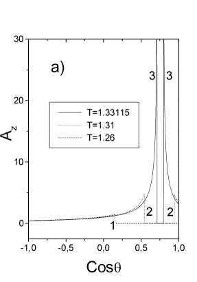
Figure 2: Time evolution of VP shock waves on the surface of the sphere S₀. $A_{z}$ is in units $e/R_{0}$, time $T=ct/R_{0}$.
a) For small times the BS shock wave occupies only back part of S₀ (curve 1). For larger times the BS shock wave begin to fill the front part of S₀ as well (curve 2). The jumps of BS shock waves are finite. The jump becomes infinite when the BS shock wave meets CSW (curve 3).
b) The amplitude of C̃erenkov’s shock wave is infinite while BS shock waves exhibit finite jumps.
c) Position of CSW and BS shock waves at the moment when CSW touches the sphere S₀ only at one point.

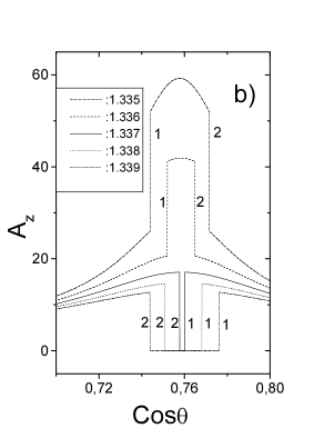
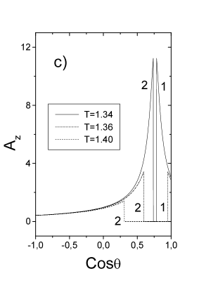
Figure 3: Further time evolution of BS shock waves on the surface of the sphere S₀.
a) The C̃erenkov post-action and BS shock waves after the moment when CSW has left S₀.
b) BS shock waves approach and pass through each other leaving after themselves the zero electromagnetic field. Numbers 1 and 2 mean BS₁ and BS₂ shock waves, resp.
c) After some moment BS shock wave begin to fill only the back part of S₀. Numbers 1 and 2 mean BS₁ and BS₂ shock waves, resp.

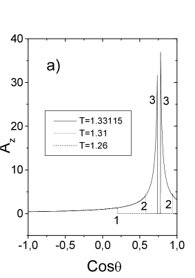
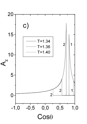
Figure 4: Time evolution of BS shock waves according to Tamm’s approximate picture.
a) The jumps of BS shock waves are finite. After some moment BS shock waves fill both the back and front parts of S₀ (curves 2 and 3).
b) Position of the BS shock wave at the moment when its jump is infinite.
c) BS shock waves pass through each other and diverge leaving after themselves the zero EMF. After some moment BS shock waves fill only the back part of S₀. Numbers $1$ and $2$ mean BS₁ and BS₂ shock waves, resp.

Figure 5: Time evolution of BS shock waves for the charge velocity ($\beta=0.7$) less the medium light velocity ($\beta_{c}=0.75$). Solid and dashed lines are related to the exact (2.1) and approximate (2.2) vector potentials.
a) BS shock waves fill only back part of S₀.
b) The whole sphere S₀ is illuminated during some time interval.
c) At later times BS again fills only the back part of S₀.

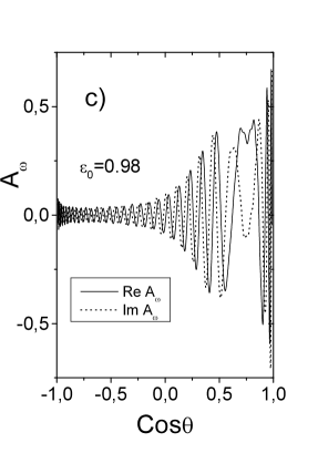
Figure 6: The real (a) and imaginary (b) parts of the VP Fourier transform (in units $e/2\pi c$) on the surface of S₀ for $\epsilon_{0}=z_{0}/R_{0}=0.1$. The radiation field differs essentially from zero in the neighborhood of the C̃erenkov critical angle $\cos\theta_{c}=1/\beta_{n}$. The solid and dotted curves refer to the exact and approximate formulae (2.1) and (2.2), resp. It turns out that a small difference of the Fourier transforms is responsible for the appearance of the C̃erenkov radiation in the space-time representation.
c) The real and imaginary parts of $A_{\omega}$ for $\epsilon_{0}=0.98$. The electromagnetic radiation is distributed over the whole sphere S₀.

Figure 7: The real (a) and imaginary (b) parts of $A_{\omega}$ on the cylinder C surface for the ratio of the interval motion to the cylinder radius $\epsilon_{0}=0.1$. The electromagnetic radiation differs from zero in the neighborhood of $z=\gamma_{n}$, that corresponds to $\cos\theta_{c}=1/\beta_{n}$ on the sphere ($z$ is in units $\rho$, $A_{\omega}$ in units $e/2\pi c$).
c) The real part $A_{\omega}$ of for $\epsilon_{0}=1$. There is no sharp radiation maximum in the neighborhood of $z=\gamma_{n}$.

Figure 8: The real part of $A_{\omega}$ for $\epsilon_{0}=10$.
a) There is no radiation maximum in the neighborhood of $z=\gamma_{n}$ and the radiation is distributed over the large $z$ interval.
b) For the small $z$ interval, $ReA_{\omega}$ evaluated according to Eq.(4.3) for $\epsilon_{0}=10$ and according to Eq.(4.5) for the infinite motion interval are indistinguishable.

References

- [1] Heaviside O 1888 Electrician (Nov. 23) p 83
- [2] []—–1889 Phil. Mag. 27 324
- [3] []—–1912 Electromagnetic Theory vol.3 (London: The Electrician)
- [4] []—–1971 Repr. ed.: (New York, Chelsea)
- [5] Cherenkov P A 1934 Dokl. Acad. Nauk SSSR 2 451
- [6] Tyapkin A A 1974 Usp. Fiz. Nauk 112 731
- [7] Kaiser T R 1974 Nature 274 400
- [8] Frank I M and Tamm I E 1937 Dokl. Acad. Nauk SSSR 14 107
- [9] Tamm I E 1939 J. Phys. USSR 1 No 5-6 439
- [10] Frank I M 1988 Vavilov-Cherenkov Radiation. Theoretical Aspects (Moscow: Nauka)
-
[11]
Afanasiev G N and Kartavenko V G 1998
J. Phys. D: Appl. Phys. 31 2760
Afanasiev G N, Kartavenko V G and Magar E N 1999 Physica B 269 95 - [12] Landau L D and Lifshitz E M 1992 Electrodynamics of Continuous Media (Oxford: Pergamon)
- [13] Lawson J D 1954 Phil. Mag. 45 748
- [14] Lawson J D 1965 Amer. J. Phys. 33 1002
- [15] Zrelov V P and Ruzicka J 1989 Chech. J. Phys. B 39 368
- [16] Zrelov V P and Ruzicka J 1992 Chech.J.Phys. 42 45
- [17] Afanasiev G N, Beshtoev Kh and Stepanovsky Yu P 1996 Helv. Phys. Acta 69 111
- [18] Afanasiev G N, Eliseev S M and Stepanovsky Yu P 1998 Proc. Roy. Soc. A 454 1049
- [19] Kobzev A P and Frank I M 1981 Yadern. Fizika 334 134
- [20] Ginzburg V L and Tsytovich V N 1984 Transition radiation and transition scattering (Moscow: Nauka) (in Russian)
- [21] []—–Ginzburg V L and Tsytovich V N 1979 Phys. Rep. 49 1
- [22] Bowler M G 1996 Nucl. Instr. and Methods in Phys. Res. A 378 463
- [23] Ginzburg V L 1940 Zh. Eksp. Teor. Fiz. 10 589
- [24] []—–1940 J. Phys. USSR 3 101
- [25] Akhiezer A I and Berestetzky V B 1981 Quantum Electrodynamics ( Moscow: Nauka)
- [26] Glauber R 1965 in Quantum Optics and Electronics (Lectures delivered at Les Houches 1964) (Eds.: DeWitt C, Blandin A and Cohen-Tannoudji C) (New York: Gordon and Breach) pp 93-279
- [27] Skobeltzyne D V 1975 C.R. Acad. Sci.Paris Ser.B 280 251 ibid.: 287
- [28] []—–1977 Usp. Fiz. Nauk 122 No 2, 295