Nonlinear waves of nuclear density

Abstract

Nonlinear excitations of nuclear density are considered in the framework of semiclassical nonlinear nuclear hydrodynamics. Possible types of stationary nonlinear waves in nuclear media are analysed using Nonlinear Schrödinger equation of fifth order and classified using a simple mechanical picture. It is shown that a rich spectrum of nonlinear oscillations in one-dimensional nuclear medium exist.

, and

1 Introduction

Nonlinear aspects of clusterization, one of the most mysterius and important problem of modern nuclear physics, are of interest due to the following reasons.

First, practically all nuclear processes which are related to clustering lead to large reconstruction of an initial nuclear system and this requires a development of new theoretical methods to describe large amplitude collective motions.

Second, the existance of clusters is a very general phenomenon. There are cluster objects in subnuclear and macro physics. Very different theoretical methods were developed in these fields. However, there are only few basic physical ideas, and most of methods deal with nonlinear partial differential equations.

Third, methods of nonlinear dynamics give us possibility to derive for nuclear physics unexpected collective modes, which can not be obtained by traditional methods of perturbation theory near some equilibrium state.

The alpha decay is the most studied process among the other possible channels of fragmentations at low energies, such as cluster radioactivity, cold fission and fusion[1]. As a rule these processes lead to a large mass transfer up to the final channel. The existence of a central region of a constant density and a well shaped surface region makes it possible to describe a clusterization in the region of nuclear surface including the neck region[2].

The alpha decay and cluster radioactivity indicate well the formation of a cluster on the surface of a large nucleus[1]. Our nonlinear approach was formulated in such a way to describe the preformation of such cluster[3]. Our model is an extension of the Bohr-Mottelson collective model[4], which allows not only the nuclear deformations which lead to collective vibrational and rotational motions, but also the creation of bumps on nuclear surface.

Nuclear density falls considerably down in a region of nuclear surface. This fact is very important due to possibility of a clusterization and other fluctuations of a nuclear density leading to instability in a surface or a neck regions[3],[5]. Recently[6] we suggested an alternative nonlinear approach, based on the currents and density algebra[7] to describe a surface interaction of a nuclei with a cluster. Starting from the hydrodinamic set of equations and using an effective Skyrme interaction, a nonlinear Schrödinger equation with fifth order term in the nonlinearity ($NoSE3-5$) has been deduced to describe in a semiclassical limit an irrotational flux of a nuclear density. In the framework of this approach an approximate way to describe surface axial symmetric interactions of a large target with a small cluster has been derived.

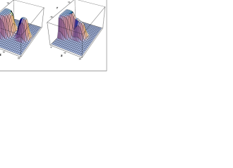
Figure 1: Surface interaction of ${}^{208}\mathop{\mathrm{Pb}}\nolimits$ and ${}^{28}\mathop{\mathrm{Mg}}\nolimits$, as a superposition of nonlinear waves of NoSE3-5

Figure 1 gives the density distributions for a surface axial symmetric (along the $z$-axes) interaction of a large target with a small cluster, as an interference of two nonlinear solutions of NoSE3-5. One can see the transition from well localized and separated initial distribution to a complicated picture, when the nucleus ${}^{28}\mathop{\mathrm{Mg}}\nolimits$ begins to be absorbed in the surface region.

Methods of nonlinear dynamics are rather unusual for traditional nuclear theory. Therefore it would be useful to understand: Why there exist nonlinear effects within linear Schrödinger picture with a many-body nuclear hamiltonian? Does there exist a way to obtain nonlinear evolution equations, starting with traditional Hamilton or Lagrange picture? How to classify possible types of solutions and to understand their physical meaning?

Within this paper we shall try to clarify these points aimed to consider simplest large amplitude oscillations of nuclear density.

The paper first presents in Sec.2 the basic scheme of our nonlinear approach to nuclear hydrodynamics. In Sec.3 it is shown how to reduce a set of hydrodynamical equations to a dimensionless nonlinear Schrödinger equation. Properties of nonlinear stationary waves are investigated in Sec.4. We give the answers to these three above questions and present a short summary in the last section .

2 Nonlinear approach to nuclear hydrodynamics

Fluid dynamical concept[8] of the nuclear medium is a traditional way to classify collective modes. Hydrodymamics gives up natural set of variables(collective currents and density) to describe any collective excitations of nuclear density. At present there are a lot of formulations of the nuclear hydrodynamical approach. We will follow the way, which is based on the current and density operators algebra[2],[7]

2.1 General scheme

For nuclear systems a usual second-quantized form of a nonrelativistic theory is defined by introducing canonically conjugated nucleon fields $\Psi({\vec{x}},\vec{\sigma},q)$, where $(q)$ denotes ($n,p$) for neutrons and protons and $\sigma=\pm$ the spin index, which satisfy the equal-time canonical anticommutation relations

$$\bigl{\{}\Psi^{+}(1),\Psi(2)\bigr{\}}_{+}=\delta(1-2),\qquad\bigl{\{}\Psi^{+}(1),\Psi^{+}(2)\bigr{\}}_{+}=\bigl{\{}\Psi(1),\Psi(2)\bigr{\}}_{+}=0.$$ (1)

In terms of these operators a nonrelativistic Hamiltonian could be defined

$${\hat{H}}_{nucl}\bigl{[}\Psi^{+},\Psi;\;U_{nucl}(\vec{x})\bigr{]}$$ (2)

with a general two-body nuclear interaction $U_{nucl}(\vec{x})$

The term ”hydrodynamics” means that we will describe the dynamical behavior of the nuclear system in a restricted space of collective variables representing the density and the nucleon current of the system:

$$\Bigl{(}\Psi^{+}({\vec{x}}),\;\Psi({\vec{x}})\bigr{)}\Longrightarrow\Bigl{(}{\hat{\rho}}({\vec{x}}),\;{\hat{j}}_{k}({\vec{x}})\Bigr{)}$$ (3)

where the index $k$ denotes the cartesian vector components.

The description of the evolution in terms of collective currents (3) requires the of use commutation relations between the collective current and density operators

$$[{\hat{\rho}}(\vec{x}),{\hat{j}}_{k}(\vec{y})],\quad[{\hat{\rho}}({\vec{x}}),{\hat{\rho}}({\vec{y}})],\quad[{\hat{j}}_{k}(\vec{x}),{\hat{j}}_{l}({\vec{y}})],$$ (4)

and their commutation relations with the hamiltonian (2)

$${\partial{\hat{\rho}}(\vec{x})\over\partial t}={1\over i\hbar}[{\hat{\rho}}(\vec{x}),{\hat{H}}_{nucl}],\qquad{\partial{\hat{j}}_{k}(\vec{x})\over\partial t}={1\over i\hbar}[{\hat{j}}_{k}(\vec{x}),{\hat{H}}_{nucl}].$$ (5)

Commutation relations (4,5) can be obtained by using the initial commutation relations (1) for nucleon quantum fields and the existing formal representation for the kinetic energy density tensor operator

$${\hat{T}}_{nk}({\vec{x}})\equiv{\nabla_{n}}\Psi^{+}({\vec{x}})\cdot{\nabla_{k}}\Psi({\vec{x}})+{\nabla_{k}}\Psi^{+}({\vec{x}})\cdot{\nabla_{n}}\Psi({\vec{x}})$$ (6)

in terms of collective currents

$${\hat{T}}^{hyd}_{kl}=({\hat{j}}_{k}{\hat{\rho}}^{-1}{\hat{j}}_{l}+{\hat{j}}_{l}{\hat{\rho}}^{-1}{\hat{j}}_{k})+{1\over 2}{\hat{\rho}}^{-1}{\nabla_{k}}{\hat{\rho}}\cdot{\nabla_{l}}{\hat{\rho}}+\mbox{const}\cdot\delta_{kl}$$ (7)

which satisfies Eqs. (5) as well.

As a result one gets a collective hydrodynamical hamiltonian

$${\hat{H}}_{nucl}\bigl{[}\Psi^{+};\;\Psi;\;U_{nucl}(\vec{x})\bigr{]}\Longrightarrow{\hat{H}}_{hyd}\bigl{[}\rho;\;\vec{j};\;T^{hyd},\;{\mathfrak{E}}[\rho,\vec{j}]\bigr{]}$$ (8)

which is equivalent to the initial nuclear hamiltonian (2) relative to the equations of motion (5). Here ${\mathfrak{E}}[\rho,\vec{j}]$ denotes effective potential term. We present the hamiltonian only schematically aimed to show the general scheme.

It is convenient to use Skyrme interaction, which gives an ansatz for an effective hamiltonian ${\hat{H}}_{hyd}\Longrightarrow\int{\d}^{3}x\/{\hat{H}}({\vec{x}})$ of a local operator in terms of densities and currents

$${\hat{H}}({\vec{x}}) = (\hbar^{2}/{2m})\tau+B_{1}\rho^{2}+B_{2}(\rho_{n}^{2}+\rho_{p}^{2})+B_{3}(\rho\tau-\vec{j}^{2})$$ (9)

$$+ B_{4}(\rho_{n}\tau_{n}-\vec{j}_{n}^{2}+\rho_{p}\tau_{p}-\vec{j}_{p}^{2})+B_{5}\rho\Delta\rho+B_{6}(\rho_{n}\Delta\rho_{n}+\rho_{p}\Delta\rho_{p})$$

$$+ B_{7}\rho^{2+\alpha}+B_{8}\rho^{\alpha}(\rho_{n}^{2}+\rho_{p}^{2})+B_{9}(\rho\nabla\cdot\vec{\Xi}+\vec{j}\cdot\nabla\times\vec{\Sigma}$$

$$+ \rho_{n}\nabla\cdot\vec{\Xi}_{n}+\vec{j}_{n}\cdot\nabla\times\vec{\Sigma}_{n}+\rho_{p}\nabla\cdot\vec{\Xi}_{p}+\vec{j}_{p}\cdot\nabla\times\vec{\Sigma}_{p})$$

$$+ B_{10}\vec{\Sigma}^{2}+B_{11}(\vec{\Sigma}_{n}^{2}+\vec{\Sigma}_{p}^{2})+B_{12}\rho^{\alpha}\vec{\Sigma}^{2}+B_{13}\rho^{\alpha}(\vec{\Sigma}_{n}^{2}+\vec{\Sigma}_{p}^{2}),$$ (10)

where the numerical coefficients $B_{i}$ and $\alpha$ are parameters of a Skyrme interaction[9].

To describe a system of nonrelativistic spin-1/2 nucleons in terms of currents requires to decompose spin-isospin density tensors to spin-scalar

$$\rho_{q}(\vec{x})\equiv\sum_{\sigma}\Psi^{+}({\vec{x}},\sigma,q)\Psi(\vec{x},\sigma,q)$$ (11)

and spin-vector densities

$$\vec{\Sigma}_{q}(\vec{x})\equiv\sum_{\sigma,\sigma^{\prime}}\Psi^{+}(\vec{x},\sigma,q)<\sigma|\vec{\sigma}|\sigma^{\prime}>\Psi(\vec{x},\sigma^{\prime},q).$$ (12)

The related currents are the spin-scalar

$$j_{k}({\vec{x}})_{q}={1\over 2i}\sum_{\sigma}\Bigl{(}\Psi^{+}({\vec{x}},\sigma,q){\nabla_{k}}\Psi({\vec{x}},\sigma,q)-{\nabla_{k}}\Psi^{+}({\vec{x}},\sigma,q)\cdot\Psi({\vec{x},\sigma,q})\Bigr{)},$$ (13)

and spin-orbital ones

$$\Xi_{k}({\vec{x}})_{q} = {1\over 2i}\sum_{\sigma,\sigma^{\prime}}\sum_{m,n=1}^{3}\varepsilon_{kmn}\Bigl{(}\Psi^{+}({\vec{x}},\sigma,q){\nabla_{m}}\Psi({\vec{x}},\sigma^{\prime},q)$$

$$- {\nabla_{m}}\Psi^{+}({\vec{x}},\sigma,q)\Psi({\vec{x},\sigma^{\prime},q})\Bigr{)}<\sigma|\sigma_{n}|\sigma^{\prime}>.$$

Among all components of the kinetic-energy-spin-tensor the most important ones are the scalars in spin and in the ordinary coordinate space

$$\tau_{q},\quad\vec{j}_{q}^{2},\quad\vec{\Sigma}_{q}^{2},\quad\nabla\cdot\vec{\Xi}_{q},$$ (15)

$$\tau=\frac{1}{2}\sum_{k}T_{kk}=\sum_{k}{\hat{j}}_{k}{\hat{\rho}}^{-1}{\hat{j}}_{k}+{1\over 4}{\hat{\rho}}^{-1}{\nabla_{k}}{\hat{\rho}}{\nabla_{k}}{\hat{\rho}}.$$ (16)

It should be noted that the operators (2.1-16) is not the complete set of spin-isospin tensor components of the current-spin-tensor and kinetic-energy-spin-tensor. The detail analysis of the equation of motion (5) for all defined densities and currents could help to clarify the situation. First of all it is necessary to define the effective hamiltonian.

In order to analyze the evolution equations (5) with the effective hydrodynamical hamiltonian (10) it is necessary: first to derive commutation relations between all components of spin-isospin current and density tensors, and their commutation relations of with all terms of hamiltonian (10) and second to provide tensor decomposition of all currents to irreducible cartesian components aimed to separate irrotational and rotational terms.

This task is rather difficult. However, in the framework of presented above general quantum hydrodynamics, one could build, in principle, a quantum approach to investigate spin-scalar, spin-vector, spin-orbital vibrational and rotational modes in nuclei. Such investigations are in progress.

3 Nonlinear Schrödinger equation

In order to check the possibilities of our approach we simplify the hamiltonian (10) aimed to describe different oscillations of isoscalar nuclear density. We assume a system of spinless and isospinless nucleons with no Coulomb, spin and spin-orbital effects ($W_{0}=0$) and effective Skyrme forces (10) ($\alpha=1$)

$$H({\vec{x}}) = \frac{\hbar^{2}}{2m}\tau+\frac{3}{8}t_{0}\rho^{2}+\frac{1}{16}t_{3}\rho^{3}+)+\frac{1}{64}(9t_{1}-5t_{2})|\nabla\rho|^{2}$$ (17)

$$+ \frac{1}{8}(3t_{1}+5t_{2})(\{\rho,\tau\}_{+}-2\vec{j}^{2}.$$

Schematic ”nonlinear density and current dependence” of kinetic energy is

$$H({\vec{x}})\Longrightarrow H_{mod}({\vec{x}})=\frac{\hbar^{2}}{2m^{*}}\sum\limits_{k=1}^{3}j_{k}\frac{1}{\rho}j_{k}+\frac{\hbar^{2}\eta^{2}}{8m^{*}}\frac{|\nabla\rho|^{2}}{\rho}+\frac{3}{8}t_{0}\rho^{2}+\frac{1}{16}t_{3}\rho^{3},$$ (18)

where the following renormalization is used

$$m \Longrightarrow m^{*}\equiv(m^{-1}+(3t_{1}+5t_{2})\rho_{N}/8\hbar^{2})^{-1},$$

$${\hbar^{2}\over 8m} \Longrightarrow {\hbar^{2}\eta^{2}\over 8m}\equiv{\hbar^{2}\over 8m}+{\rho_{N}\over 64}(9t_{1}-5t_{2}).$$ (19)

$H_{mod}$ form Eq. (18) is the simplest hamiltonian which includes the ”collective” kinetic energy, ”Weizsäcker” kinetic part which includes the quantum and other gradient terms and the ”potential” energy, containing effective two-body attractive term and three-body imitation of Pauli principle.

In classical hydrodynamics[10], the fundamental variables are the local density $\rho(\vec{x})$ and the fluid velocity $\vec{v}(\vec{x})$ from which the quantum current density can be defined by the anticommutator[11]

$$\hat{j}_{i}(\vec{x})={m\over 2\hbar}\{{\hat{\rho}}(\vec{x}),\hat{v}_{i}(\vec{x})\}_{+}.$$ (20)

Using the definition (20) and the commutative relations between density and current operators (4) one derives velocity-density and velocity-velocity commutative relations

$$[{\hat{v}}_{k}(\vec{x}),{\hat{\rho}}({\vec{y}})],\qquad[{\hat{\rho}}({\vec{x}}),{\hat{\rho}}({\vec{y}})],\qquad[{\hat{v}}_{i}(\vec{x}),{\hat{v}}_{j}(\vec{y})].$$ (21)

To classify the type of motions in the cartesian coordinate space it would be convenient to provide tensor decomposition of the operator vector field

$$\hat{v}_{k}(\vec{x})=\nabla_{k}\hat{\Phi}_{pot}(\vec{x})+curl_{k}(\hat{\vec{A}}),\qquad div(\hat{\vec{A}})=0,$$ (22)

into a sum of potential $(\hat{\Phi}_{pot}(\vec{x}))$ and solenoidal $(\hat{\vec{A}})$ fields by using the Helmholtz theorem (see, e.g., ref.[12] vol. 1).

In the following we shall consider the equations of motion (5) with the hamiltonian $H_{mod}$ (18). First it is convenient to use the scale transformations [7]

$$\vec{x}\equiv(\hbar\eta/m^{*}c_{s})\/\vec{x}^{{}^{\prime}},\qquad t\equiv(m^{*}c_{s}^{2}/\hbar)\/\tau,$$ (23)

$$v_{k}(\vec{x})=c_{s}U_{k}(\vec{x}^{\prime}),\qquad\rho(\vec{x},t)\equiv\rho_{N}\/n^{2}(\vec{x}^{\prime},\tau).$$ (24)

where $c_{s}$ is the sound velocity in nuclear matter

$$c_{s}\equiv\bigl{(}{1\over m^{*}}\rho^{2}{\delta^{2}({\mathfrak{E}}/\rho)\over\delta\rho^{2}}|_{\rho=\rho_{N}}\bigr{)}^{1/2}$$ (25)

The scale transformation (23,24) makes it possible to separate the general effects related to nonlinearity in the hamiltonian (18) (a polinomial in density) from effects related to a choice of parameters of interaction, which define only scales factors: effective length wave ($\hbar\eta/m^{*}c_{s}$ ), the density of nuclear matter $\rho_{N}$, the sound velocity in nuclear matter $c_{s}$ and the time factor ($m^{*}c_{s}^{2}/\hbar$).

Hamiltonian (18) can be cast in the following form

$$H_{mod}=\rho_{N}\left(\frac{\hbar\eta}{m^{*}c_{s}}\right)^{3}m^{*}c_{s}^{2}\int{\d}^{3}x^{\prime}\left(\sum\limits_{k=1}^{3}\frac{U_{k}nU_{k}}{2}+\frac{|\nabla n|^{2}}{8n}-n^{2}+\frac{1}{2}n^{3}\right).$$ (26)

Now the continuity and Euler operator equations (5) can be reduced to the following set of the dimensionless equations of motion

$$\frac{\partial n(\vec{x}^{\prime})}{\partial\tau}=-\frac{1}{2}\sum\limits_{k=1}^{3}\frac{\partial}{\partial x_{k}^{\prime}}\{{n(\vec{x}^{\prime}),U_{k}(\vec{x}^{\prime})}\}_{+},$$ (27)

$$\frac{\partial U_{k}(\vec{x}^{\prime})}{\partial\tau} = \frac{1}{2}\left(\left(\vec{U}\times curl\vec{U}\right)_{k}-\left(curl\vec{U}\times\vec{U}\right)_{k}\right)$$ (28)

$$- \frac{1}{2}\frac{\partial}{\partial x_{k}^{\prime}}\left(\vec{U}^{2}+\frac{\Delta n}{2n}-\frac{|\nabla n|^{2}}{4n^{2}}-4n(\vec{x}^{\prime})+3n^{2}(\vec{x}^{\prime})\right).$$

Taking into account the velocity-velocity and velocity-density commutative relations (20-21) and the operator Helmholtz theorem (22) we obtain the following decomposition of the dimensionless velocity operator:

$${\hat{U}}_{k}(\vec{x})=\frac{\partial{\hat{\Phi}}(\vec{x})}{\partial x_{k}}+{\hat{R}}_{k}(\vec{x}),\qquad div\vec{R}=0,\qquad\vec{\hat{\zeta}}=curl\vec{\hat{R}},$$ (29)

into potential and pure rotational currents.

Considering only the vibrational type of motion and neglecting their possible connection with rotational modes ($\vec{\hat{\zeta}}=0,\,{\hat{R}}_{k}\to 0$) the commutation relations between density and potential velocity are reduced to the canonical boson form

$$[\hat{n}(\vec{x}),\hat{\Phi}(\vec{y})]=i\delta(\vec{x}-\vec{y}),\qquad[\hat{\Phi}(\vec{x}),\hat{\Phi}(\vec{y})]=0,\qquad[{\hat{n}}({\vec{x}}),{\hat{n}}({\vec{y}})]=0,$$ (30)

which give it possible to treat (if it is no rotation ($R_{k}=0$)) the evolution via $H_{mod}$ as nonlinear operator anharmonical picture.

In the semiclassical limit the two hydrodynamical equations of motion (27,28) in the case of irrotational flow (29,30) can be cast in the form of one nonlinear Schrödinger equation

$$i{\psi_{\tau}}=-\Delta\psi-4\mid\psi\mid^{2}\/\psi+3\mid\psi\mid^{4}\/\psi$$ (31)

for a complex function $\psi$

$$n(\vec{x},\tau)=\mid\psi(\vec{x},\tau)\mid^{2},\qquad\Phi(\vec{x},\tau)=\arg\psi(\vec{x},\tau).$$ (32)

Eqs. (31,32) become transparent if we recall the well-known formal analogy of quantum mechanics to fluid mechanics[8]. However one should keep in mind that in formulaes (31,32) all variables are collective ones and the effective potential is defined by a first functional derivative of effective interaction on density.

4 The one-dimensional nonlinear waves

Let us consider the stationary (travelling) solutions of the one-dimension (in the cartesian coordinate space) nonlinear Schrödinger equation (31). These solutions take the usual form

$$\psi(r,\tau)\equiv\psi(x)\exp\bigl{(}i(\lambda-v^{2}/2)\tau+ixv+\sigma_{0})$$ (33)

where $r=x-v\tau-r_{0}$. The parameters $r_{0},\sigma_{0},v$ are the initial position of the center of the wave, the initial phase shift and the initial velocity.

The function $\psi(x)$ is the solution of the nonlinear Schrödinger equation

$$\psi_{xx}-\lambda\psi+4\psi^{3}-3\psi^{5}=0.$$ (34)

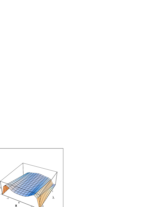
Figure 2: Dependence of ”potential” $V(\psi)$ on $\psi$ and and $\lambda$

To analyze different solutions of Eq. (34) we will exploit its simple mechanical analog, in which a macroscopic point ”particle” of unit mass is moving under a conservative ”force”

$$F(\psi)=\lambda\psi-4\psi^{3}+3\psi^{5}\equiv-\frac{\partial V(\psi)}{\partial\psi},$$ (35)

where the ”potential” (see Figure 2) is taken as

$$V(\psi)=-\frac{\lambda}{2}\psi^{2}+\psi^{4}-\frac{1}{2}\psi^{6},$$ (36)

with $\psi$ as a ”particle position” and $x$ its ”time”.

Eq. (34) after being multipled by $\psi_{x}$ , can be one time integrated. The result is

$$\psi_{x}=\pm\sqrt{2(E-V(\psi))},\qquad E=V(\psi)+\frac{1}{2}\psi_{x}^{2}$$ (37)

where the constant of integration ($E$) is considered to be the ”energy”. Eq. (37) is just the energy conservation law in the analog ”particle” problem. The parameter ($\lambda$) defines the ”potential” profile and the ”energy” ( $E$ ) defines the ”particle” motion.

Figure 2 gives a gross ”potential” picture. We show a detail set of ”potentials” $V(\psi)$ for different values of the parameter ($\lambda$ ) in Figs. 3 . The ”potential” $V(\psi)$ (36) vanishes at the points

$$\psi=\{0,\quad\pm P_{1}=\pm\sqrt{1-\sqrt{1-\lambda}},\quad\pm P_{2}=\pm\sqrt{1+\sqrt{1-\lambda}}\}$$ (38)

(see Figure 3 ($\lambda=0.5$)).

The equilibrium points of motion $F(\psi)=-\partial V(\psi)/\partial\psi=0$ are given by

$$\psi=\{0,\quad\pm P_{3}=\pm\sqrt{\frac{2-\sqrt{4-3\lambda}}{3}},\quad\pm P_{4}=\pm\sqrt{\frac{2+\sqrt{4-3\lambda}}{3}}\}$$ (39)

(see Figs.3 ($\lambda=0.9$)). For an nonpositive $\lambda\leq 0$ a finite amplitude motion is possible only for $0<E<V(P_{4})$ and $|\psi(0)|<P_{4}$ (see Figs.3 ($\lambda=0.0$)). For $0<\lambda<1$ there exist a finite amplitude motion eith different types for the three regions of the ”energy” $\{V(P_{3})<E<0,\;E=0,\;0<E<V(P_{4})\}$ (see Figs.3 ($\lambda=0.5,0.9$)). This is the most interesting case and in the following we will consider it in detail. For $\lambda=1$ the ”barriers” $V(-P_{4})=V(0)=V(P_{4})=0$ (Figs.3 ($\lambda=1.0$)). A finite amplitude motion for $1\leq\lambda<4/3$ is possible only for the negative ”energy” $V(P_{3})<E<0$ (Figs.3 ($\lambda=1.1$)). For $\lambda>4/3$ (see Figs. 3 ($\lambda=1.5$)) any motion of a finite amplitude is impossible. A ”particle” comes away from the origin for any energy.

Eq. (34) is an ordinary differential equation of a second order. For any set of initial values $\psi(x_{0}),\;\psi_{x}(x_{0})$ at initial ”time” $x_{0}$ one can obtain, in principle, the solution of Eq. (34) numerically. We will restrict ourselves only to stationary waves of a finite amplitude. This means that for a given $\lambda$ the ”energy” is less than the maximum ”barrier” value ( $E<V(\pm P_{4}))$. Therefore it is convenient to select an ”initial point” $x_{0}$, as the point at ”potential” profile in which

$$E=V(\psi_{0}),\qquad\psi_{x}(x_{0})=0,\qquad\psi_{0}\equiv\psi(x_{0}).$$ (40)

Because of the ”energy conservation” the $E$ parameter is related to the wave amplitude $\psi(0)$.

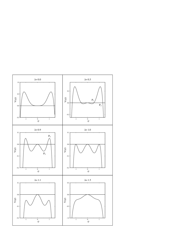
Figure 3: Dependence of a ”potential” $V(\psi)$ on $\psi$ for different parameters $\lambda$

A localized soliton like solution is the nodeless solution of Eq. (34) under the following boundary condition

$$\psi(\infty)=\psi_{x}(\infty)=\psi_{x}(0)=0.$$ (41)

This corresponds to a special case with $E=0$. Soliton like solution exists if $0<\lambda<1$. A ”particle” starts motion in the point $P_{1}$ or $-P_{1}$ (see Eq. (38)) and comes to origin.

Figure 4: Soliton -like solutions of NoSE3-5 for different values of the parameters $\lambda$

In Figures 4 we present the soliton like solutions for a few values of the parameter ($\lambda$). There exist an analytical form of this soliton like solution[7]

$$\psi(x)=(\lambda/(1+(1-\lambda)^{1/2}\cosh(2\lambda^{1/2}r))^{1/2}.$$ (42)

which looks like a symmetrized Fermi-distribution

$$\psi(x)=\sqrt{\frac{\sinh({\mathfrak{R}}/{\mathfrak{D}})}{\cosh({\mathfrak{R}}/{\mathfrak{D}})+\cosh(x/{\mathfrak{D}})}}$$ (43)

where the ”radius”

$${\mathfrak{R}}=\frac{1}{2\sqrt{\lambda}}{\rm arctanh}(\sqrt{\lambda}).$$ (44)

and the ”diffuseness”

$${\mathfrak{D}}=\frac{1}{2\sqrt{\lambda}}$$ (45)

are defined by the parameter ($\lambda$).
The parameter $\lambda$ is the chemical potential defined by the ”particle number”

$$N=\int_{-\infty}^{\infty}\d x\;\psi(x)^{2},\qquad N={\rm arctanh}(\sqrt{\lambda})$$ (46)

Figure 5: Set of stationary nonlinear waves of NoSE3-5

It is useful to note also the following features of this soliton like solution. First for a small ”particle number” the solution looks like a solution of a cubic nonlinear Schrödinger equation. Second, for an intermediate and large ”particle numbers” the ”radius” (44) is increased (see Figs.4). Third, there exist an internal region of approximate constant ”density” and a ”surface region” of a ”constant” diffuseness (see Eqs. (44,45) and Figs.4(c,d)).

In Figures 5 we present possible periodical and aperiodical solutions of Eq. (34) for $\lambda=0.5$. The corresponding ”potential” is represented in Figs.3 ($\lambda=0.5$). One can see small oscillations with a positive amplitude in the ”well” for ($V(P_{3})<E<0$) (Figs.5(a)) These oscillations became distorted more and more, as $E\to 0-\epsilon$, where $\epsilon$ is an infinite small positive value (see Figs.5(b,c)). For $E=0$ we have the exact soliton like solution (Figs.5(d)). There are nonlinear waves of positive and negative apmlitude, as $E\to V(P_{3})+\epsilon$, (see Figs.5(e,f)). These waves look like quasi-trigonometrical functions (see Figs.5(g)), as $\lambda$ changes from small positive values to the ”barrier” $V(P_{4})$.

Periodical waves became distorted more and more, as $E\to V(P_{4})-\epsilon$. In Figs.5(h,i) one can see a transition from a well-defined periodical structure to an aperiodical one.

There is a region of semi ”shock” wave with the well defined sharp ”front” (see Figs.5(i)). ”Front” moves to the infinity and, in this case, we have the constant solution in coordinate space when an ”energy” is equal to the ”barrier” ($E=V(P_{4})$) (see Fig.5(j)), describes a one-dimensional nuclear matter.

The above solutions were obtained numerically. However it is possible to get also analytical solutions for few special cases. First it shoud be noted that it is possible to write a formal solution of Eq. (37)

$$\int_{\psi_{0}}\frac{{\psi}\,\d\psi}{\sqrt{2(E-V(\psi))}}=\pm\int_{x_{0}}{x}\d x$$ (47)

for any types of nonlinearity, i.e. for any ”potential” $V(\psi)$.

In our case $V(\psi)$ is given by a symmetrical polinomial of six order in $\psi$ (36). The substitution $Z\equiv\psi^{2}$ reduces equation (34) to the following form

$$Z_{x} = \pm 2\sqrt{Z(2E+\lambda Z-2Z^{2}+Z^{3})}$$ (48)

$$\equiv \pm 2\sqrt{Z(Z-Z_{1})(Z-Z_{2})(Z-Z_{3})}$$

The expression under the square root of the Eq. (48) is a polinomial of fourth degree. One of the roots is $Z=0$ the other three ones being defined by $E,\;\lambda$ parameters.

The following solution of Eq. (48) exists also in the case of $E=0,\lambda=0$

$$\frac{\sqrt{Z(Z-2)}}{2Z}=\pm 2x\qquad Z(x)=\frac{2}{1-4x^{2}}$$ (49)

where the constants of integration are omitted. This solution has a pole at $x=\pm 2$, and it does not describe a finite solution.

For very few special cases Eq. (48) can be integrated analytically in Jacobian elliptic functions. These functions are quite similar to the trigonometric functions. One can find in the book[13] the complete set of twelve different Jacobian ellipic functions and the coresponding form of the differential equation. If it is possible to reduce Eq. (48) by a linear transformation $(Z,x)\to(z,u)$ to the one of these forms, then the solution of (48) can be cast as the related Jacobi elliptic function. The explicit form of the solution is determined by the constants $\lambda,E$ and boundary conditions.

5 Summary

We give the following answers to the three questions formulated in Introduction.

Nonlinear problems exist within a linear Schrödinger picture with a many-body nuclear hamiltonian as the result of the reduced description in a restricted space of collective degrees of freedom. In Sections 2 and 3 the way to derive the Nonlinear Schrödinger equation for a collective motion is presented. The logic of our approach corresponds to the logic of any microscopic or semimicroscopic theory of collective nuclear motion, namely, one first selects a space of certain collective variables (3) and their commutation relations (4). Then seeks an expresssion for the collective Hamiltonian (8) in terms of the chosen collective variables to reproduce the commutation relations (5) of the original many-particle Hamiltonian and the collective operators. The hydrodynamical collective hamiltonian (8) is equivalent to the initial Hamiltonian (2) only with respect to the equations of motion (5) for the collective operators (2). The present approach is the realization for nuclear physics of the general problem how to formulate nonrelativistic quantum mechanics in terms of collective current operators. The currents (3) can be considered as fundamental dynamical variables rather than the underlying canonical fields (1). The main emphasis of this type of theory is the algebraic structure of the equal-time current-current commutation relations (4). The motivation for initiating such a program was due to the fact that most of the interesting physical quantities can be expressed in terms of currents and densities. It is important for nuclear physics because the density and velocity distributions are usual variables to analyse the dynamics of heavy ion collisions (see the recent papers[14],[15] and the references therein).

In the present paper, possible types of stationary nonlinear waves in nuclear media are analyzed in the framework of Nonlinear Schrödinger equation of fifth order and classified using a simple mechanical picture. It is shown that a rich spectrum of nonlinear oscillations in one-dimensional isoscalar nuclear matter exist.

References

- [1] A. Sãndulescu and W. Greiner, Rep. Prog. Phys. 55, 1423 (1989).
- [2] V. G. Kartavenko, Phys. Part. Nucl. 24 619 (1993).
- [3] A. Ludu, A. Sãndulescu and W. Greiner, Int. J. Mod. Phys. E1 169 (1992).
- [4] J. M. Eisenberg and W. Greiner, Nuclear Models (Collective and Single-Particle Phenomena, Vol.1) (North Holland Publ. Comp. Amsterdam), 1970.
- [5] V. G. Kartavenko, J. Phys. G: Nucl. Part. Phys. 19 L83 (1993).
- [6] V. G. Kartavenko, A. Ludu, A. Sãndulescu and W. Greiner, Int. J. Mod. Phys. E5 329 (1996).
- [7] V. G. Kartavenko, Sov. J. Nucl. Phys. 40 240 (1984).
- [8] E. Madelung, Z.Phys. 40, 332 (1926).
- [9] P. Bonche, H. Flocard and P. H. Heenen, Nucl. Phys. A467 115 (1987).
- [10] H. Lamb, Hydrodynamics (New York: 6th Edition Dover Publications) (1932).
- [11] B. T. Geilikman, Doklady AN USSR (in russian) 94 199 (1954).
- [12] P. M. Morse and H. Feshbach, Methods of Theoretical Physics (New York: McGraw-Hill) 1953.
- [13] M. Abramowitz and I. A. Stegun, Handbook of Mathematical Functions (Dover Publications, Inc., New Youk) Ch.16 (Milne-Thompson L.M.) p.56
- [14] V. G. Kartavenko, K. A. Gridnev, J. Maruhn and W. Greiner, J. Phys. G: Nucl. and Part. Phys. 22 (1996) L19
- [15] A. Ludu, A. Sãndulescu and W. Greiner, J. Phys. G: Nucl. Part. Phys. 23 343 (1997).