Probing the width of compound states with rotational gamma rays

Abstract

The intrinsic width of (multiparticle-multihole) compound states is an elusive quantity, of difficult direct access, as it is masked by damping mechanisms which control the collective response of nuclei. Through microscopic cranked shell model calculations, it is found that the strength function associated with two-dimensional gamma-coincidence spectra arising from rotational transitions between states lying at energies $>$ 1 MeV above the yrast line, exhibits a two-component structure controlled by the rotational (wide component) and compound (narrow component) damping width. This last component is found to be directly related to the width of the multiparticle-multihole autocorrelation function.

PACS: 21.10.Ky, 21.10.Re, 21.60.-n, 23.20.Lv, 25.70.Gh

Keywords: compound damping width, rotational damping, high spin states, quasi-continuum gamma spectra.

In deformed nuclei, the observed discrete rotational bands are often successfully described as states of a cranked mean field [1]. For fixed angular momentum and increasing excitation energy, the residual interaction not included in the mean field will eventually generate compound states, which are superpositions of the many-particle many-hole mean field states. As a result, each basis band state $|{\mu}\rangle$ becomes distributed over the compound states $|{\alpha}\rangle$ within an energy interval known as the compound state damping width $\Gamma_{\mu}$ [2, 3, 4].

The quantity $\Gamma_{\mu}$ plays a central role in the study of basic nuclear phenomena, like the statistical and chaotic features of energy levels [5, 6, 7], or the damping of collective vibrations [8, 9]. However, it also appears to be inaccessible by direct experimental means, since it is essentially not possible to excite a pure many-particle many-hole state. We shall demonstrate that the spectrum of collective E2-gamma rays emitted by the compound states built out of rotational bands carries information about $\Gamma_{\mu}$. This is true also for the unresolved gamma rays, which are far too weak to allow for construction of a level scheme with present experimental techniques.

Although rotational damping is a phenomenon which is independent of compound damping, being controlled by fluctuations in the alignment of the single-particle states, the occurence of compound states in rotational nuclei is usually accompanied by damping of rotational motion [3, 4, 10, 11, 12]. In what follows we shall study the interplay between these two independent phenomena, namely rotational damping and compound damping, as a function of spin and excitation energy, making use of a cranked shell model which has been applied earlier to the study of rotational damping and of the statistical properties of spectral fluctuations and level distances [13, 14, 15]. The calculations have been performed for the rare-earth nucleus ¹⁶⁸Yb, for which the quasi-continuum gamma spectrum has been analyzed in detail experimentally. The shell model Hamiltonian, consisting of the cranked Nilsson mean-field and the surface-delta interaction acting as the residual two-body force, is diagonalized using the lowest 2000 many-particle many-hole configurations based on the cranked Nilsson single-particle orbits for each value of average angular momentum $I$ and the parity $\pi$. This provides the lowest 600 energy levels for each $I^{\pi}$ covering an energy range up to about 2.5 MeV above the yrast line. (See ref. [15] for further details). In the calculation, rotational damping sets in at about 1 MeV above the yrast line (in agreement with experiments) as a consequence of the spreading of the unperturbed rotational bands having specific and simple shell model configurations in a rotating deformed mean-field. Above the onset energy and up to a few MeV, two-particle two-hole (2p2h) and three-particle three-hole (3p3h) configurations are the dominant configurations forming the compound states. The compound damping width $\Gamma_{\mu}$ of interest is the spreading width of these many-particle many-hole ($n$p-$n$h) configurations (which we label by $|{\mu}\rangle$) over the compound states $|{\alpha}\rangle$.

The spreading width $\Gamma_{\mu}$ is, by definition, the energy interval over which the strength of a given $\left|\mu\right>$ state is distributed. The distribution may formally be represented by the strength function [2]

$$S_{\mu}(E)=\sum_{\alpha}|\langle{\alpha}|{\mu}\rangle|^{2}\delta(E-(E_{\alpha}-\bar{E}_{\mu})),$$

where $\langle{\alpha}|{\mu}\rangle$ is the amplitude of the $n$p-$n$h $\left|\mu\right>$-state contained in the compound level $|{\alpha}\rangle$ of energy $E_{\alpha}$, while $E$ refers to the energy relative to the centroid $\bar{E}_{\mu}$ of the strength distribution. Calculated examples of the above function are shown in Fig.1(a). It is noted that the strength spreads over a limited number of energy levels, and never shows a smooth profile, because of the discreteness of the energy levels. Furthermore, the strength function varies strongly from state to state. A smoother behaviour is obtained by taking the average of $S_{\mu}(E)$ over all $|{\mu}\rangle$ states lying within an energy bin and spin interval, trimming the delta functions with a smoothing function (in the present analysis we use a Strutinsky’s Gaussian function with the Laguerre orthogonal polynomial of 10 keV width). The averaged strength function $\left<S_{\mu}(E)\right>$ thus obtained is shown in Fig.1(b). It is customary to define the spreading width by the FWHM of $\left<S_{\mu}(E)\right>$, denoted by $\Gamma_{\mu}^{s}$, with the label $s$ referring to the average strength function.

Another definition of the spreading width is possible, making use of the autocorrelation function applied to the strength function $S_{\mu}(E)$ of individual $n$p-$n$h states. The autocorrelation function

$$C_{\mu}(e)=\int S_{\mu}(E+e)S_{\mu}(E)dE$$

expresses the probability of pairwise strengths in $S_{\mu}(E)$ being located relative to another at the energy distance $e$. If the strength function $S_{\mu}(E)$ were of Breit-Wigner shape of width $\Gamma$, the autocorrelation function would also have a Breit-Wigner shape, displaying twice the width as that of the original strength functions. The autocorrelation function $C_{\mu}(e)$ has a physical interpretation as the Fourier transform of the “survival probability” $P_{\mu}(t)=|\left<\mu|\mu(t)\right>|^{2}$, which measures the probability of remaining in the state $\left|\mu\right>$ during its time evolution $\left|\mu(t)\right>=e^{-iHt}\left|\mu\right>$. For the case of the Breit-Wigner strength function, $P_{\mu}(t)$ decays exponentially with a decay constant given by $\hbar/\Gamma$. We average $C_{\mu}(e)$ over many $\left|\mu\right>$ states in an energy bin and spin interval and make the same smoothing as described above for the strength function $S_{\mu}(E)$. It is remarked that the autocorrelation function $C_{\mu}(e)$ contains a delta-function peak at $e=0$ proportional to $\sum_{\alpha}|\langle{\alpha}|{\mu}\rangle|^{4}$, which we remove in the following analysis, since this peak corresponds to the asymptotic value of $P_{\mu}(t)$ at the $t\rightarrow\infty$ limit. The resultant autocorrelation function $\left<C_{\mu}(e)\right>$ is shown in Fig.1(c). The correlational spreading width can be defined as half the value of FHWM of the autocorrelation function $\left<C_{\mu}(e)\right>$. In order to distinguish from the previous definition $\Gamma_{\mu}^{s}$ in terms of the averaged strength function, we denote this new quantity $\Gamma_{\mu}^{corr}$ making use of the label ’corr’.

The most immediate feature observed in the calculated autocorrelation function $\left<C_{\mu}(e)\right>$ as compared to the average strength function $\left<S_{\mu}(E)\right>$ is its narrower profile. Correspondingly, the correlational spreading width $\Gamma_{\mu}^{corr}=41$ keV extracted from the autocorrelation function shown in Fig.1(c) is about a factor four smaller than $\Gamma_{\mu}^{s}$.

In order to understand this difference it is useful to look at the details of the strength functions associated with ’individual’ $n$p-$n$h states (cf. Fig.1(a)). The strength distribution of individual states is typically clustered within a narrower energy interval than that associated with the average strength function $\left<S_{\mu}(E)\right>$ (cf. e.g. the strength function associated with the 74-th and 75-th $n$p-$n$h states of angular momentum and parity $I^{\pi}=40^{+}$). Also, the position of the dominant strengths deviates from the centroid position $(E=0)$ and varies between different $\mu$ configurations. This variation results in a broad profile of the average strength function $\left<S_{\mu}(E)\right>$. In contrast, the width of the individual autocorrelation functions $C_{\mu}(e)$ reflects the clustering of strengths. Thus, the averaged autocorrelation $\left<C_{\mu}(e)\right>$ forms a peak around $e=0$ whose width is not influenced by the energy shift of the dominant strength, which only gives rise to wide tails stretching out to large positive and negative energies. Since the energy shift does not imply spreading nor influence the survival probability, we posit that the correlational width $\Gamma_{\mu}^{corr}$ is more appropriate to characterize the spreading width than the quantity $\Gamma_{\mu}^{s}$. The difference between $\Gamma_{\mu}^{corr}$ and $\Gamma_{\mu}^{s}$ decreases gradually with increasing excitation energy of the $n$p-$n$h states. However, we find from a calculation using an extended basis of 6000 $n$p-$n$h states that $\Gamma_{\mu}^{corr},\Gamma_{\mu}^{s}=133,305$ keV for the levels $\#1800-\#2100$ at $I=40,41$ indicating that around $U\approx 3$MeV there is a difference of about a factor of 2 between these two quantities. At this energy, while the strength of individual $|{\mu}\rangle$ states is spread over several hundreds of levels, the distribution still displays, in most cases, a strong clusterization around a few big peaks, and does not show a smooth Breit-Wigner distribution.

Our studies have also shown that the difference found between $\Gamma_{\mu}^{corr}$ and $\Gamma_{\mu}^{s}$ is related to the nature of the two-body residual interaction used in the calculations (cf. Figure 2). Replacing the surface delta interaction (SDI) by a volume-type delta force ($V(1,2)=v_{\tau}\delta(\vec{x}_{1}-\vec{x}_{2})$), the ratio between $\Gamma_{\mu}^{s}$ and $\Gamma_{\mu}^{corr}$ is as large as for the SDI. On the other hand, using a random two-body interaction for which the two-body matrix elements $v_{ijkl}=\left<ij|V(1,2)|kl\right>$ are replaced with Gaussian random numbers, it is found that the resulting $\Gamma_{\mu}^{corr}$ approximately coincides with $\Gamma_{\mu}^{s}$, irrespective of the average strength of the matrix elements.

Before discussing the physics which is at the basis of these results, it is reasonable to mention that the SDI or the delta residual interaction are a better representation for nuclear structure calculations at moderate excitation energies above the yrast line, of the residual interaction acting among nucleons, than that provided by a random force. It is well known that the SDI (or the delta interaction) and the random interaction differ dramatically in the statistical distribution of two-body matrix elements $v_{ijkl}$. In fact, the distribution $P(v_{ijkl})$ for the SDI, plotted in Fig.3 (and for the delta interaction, not shown here), exhibits a strong skewness. In other words, it has a significant excess for large matrix elements $|v_{ijkl}|>60$ keV compared with a Gaussian distribution having the same r.m.s value $\sqrt{<v_{ijkl}^{2}>}=19$ keV. In fact, the large matrix elements of the SDI contribute to the r.m.s. value as much as the small ones $|v_{ijkl}|<60$ keV, as seen in the right panel plotting $v_{ijkl}^{2}P(v_{ijkl})$, although large matrix elements appear quite rarely (only 2% of the total number of matrix elements). On the other hand, the Gaussian random interaction contains no such contribution from large matrix elements. The role of the large (and rare) matrix elements of the SDI can be made even clearer through a calculation of $S_{\mu}(E)$ and $C_{\mu}(e)$ carried out with a truncated SDI, where only the small matrix elements $|v_{ijkl}|<60$ keV are kept. This truncation has a significant effect on the calculated average strength function $\left<S_{\mu}(E)\right>$, diminishing $\Gamma_{\mu}^{s}$ to less than half of its original value. On the other hand, the average autocorrelation function $\left<C_{\mu}(e)\right>$ remains almost unchanged, keeping the original value of $\Gamma_{\mu}^{corr}$ (cf. Fig.2). The large matrix elements of the SDI tend to shift the energies of the levels, rather than mixing the $n$p-$n$h configurations around the energy shell. As a consequence, they have a strong effect on $\Gamma_{\mu}^{s}$, but not to $\Gamma_{\mu}^{corr}$.

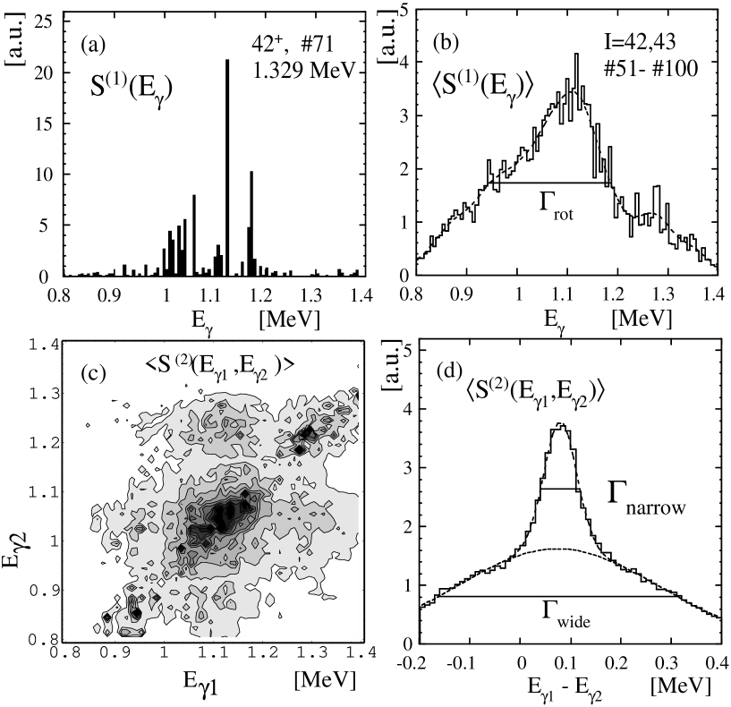
Figure 4: (a) The calculated one-step strength function $S_{\alpha}^{(1)}(E_{\gamma})$ for a typical compound level, the 71-st 42⁺ states lying at 1.329 MeV above the yrast line. (b) The average one-step strength function $\left<S_{\alpha}^{(1)}(E_{\gamma})\right>$ for the levels in the energy bin including the 51-st to 100th lowest levels (for each $I^{\pi}$) at spin $I=42,43$. The associated width is the rotational damping width $\Gamma_{rot}$. (c) The average two-step strength function $\left<S_{\alpha}^{(2)}(E_{\gamma 1},E_{\gamma 2})\right>$ calculated for the same levels. (d) Its projection on the $E_{\gamma 1}-E_{\gamma 2}$ axis. The width $\Gamma_{narrow}$ and the intensity $I_{narrow}$ of the narrow component are extracted fitting the shape of the projection with two Gaussians.

Seen from the perspective of gamma decay cascades, the strengths $S_{\mu}(E)$ and $C_{\mu}(e)$ are zero-step functions, describing the coupling of $n$p-$n$h states locally at one value of the angular momentum $I$. On the other hand, the gamma transitions $\left|\alpha(I)\right>\stackrel{{\scriptstyle E_{\gamma}}}{{\longrightarrow}}\left|\alpha^{\prime}(I-2)\right>$ taking place between compound energy levels of angular momenta $I$ and $I-2$ are described by the one-step E2 strength function $S_{\alpha}^{(1)}(E_{\gamma})$ while the consecutive gamma transitions $\left|\alpha(I)\right>\stackrel{{\scriptstyle E_{\gamma 1}}}{{\longrightarrow}}\left|\alpha^{\prime}(I-2)\right>\stackrel{{\scriptstyle E_{\gamma 2}}}{{\longrightarrow}}\left|\alpha^{\prime\prime}(I-4)\right>$ are described by the two-step strength functions $S_{\alpha}^{(2)}(E_{\gamma 1},E_{\gamma 2})$. Figure 4 shows examples of these two types of strength functions. Individual one-step strength functions $S_{\alpha}^{(1)}(E_{\gamma})$ display considerable fine structures (Fig.4(a)) which vary for different initial $\left|\alpha\right>$ states while their average over many states becomes a rather featureless function(Fig.4(b)), from which one can extract only the rotational damping width $\Gamma_{rot}$. The two-step function $S_{\alpha}^{(2)}(E_{\gamma 1},E_{\gamma 2})$, on the other hand, exhibits a two-component structure even after averaging over many states as shown in Fig.4(c,d) and discussed earlier [15, 16, 17]. Projected on the $E_{\gamma 1}-E_{\gamma 2}$ axis, the two components are characterized by wide and narrow widths, $\Gamma_{wide}$ and $\Gamma_{narrow}$ (cf. Fig.4(d)). On the basis of our results for the autocorrelation function of the zero-step mixing discussed above, we shall show below that the narrow component in the two-step function can be given a more precise interpretation as a doorway phenomenon related to the compound damping width. Thus, the two-step function carries information on the compound damping width $\Gamma_{\mu}$ as well as on the rotational damping width $\Gamma_{rot}$.

The admixture of $n$p-$n$h states $|{\mu}\rangle$ into each compound state $|{\alpha}\rangle$ produces strengths $|\langle{\alpha}|{\mu}\rangle^{2}|$ which fluctuate strongly, even at high excitation energies above the yrast line ($\approx$ 3 MeV), where their distribution is expected to approach a Porter-Thomas shape [14]. E2 transitions from a given state $|{\alpha}\rangle$ at angular momentum $I$ will single out states $|{\alpha^{\prime}}\rangle$ at $I-2$, which contain strong components of the same $|{\mu}\rangle$ states as in $|{\alpha}\rangle$, and this will also take place in the second transition to $I-4$. In this sense, the dominant components $|{\mu(I-2)}\rangle$ at the midpoint of the two consecutive decay steps act as ”doorway states” in the two-step cascade. If the spreading width $\Gamma_{\mu}$ of the ”doorway states” is considerably smaller than the rotational damping width $\Gamma_{rot}$, the E2 strength distribution will exhibit structures which are associated with the ”doorway states” having the rotational energy correlation, and smeared by $\Gamma_{\mu}$ in both of the decay steps. Assuming a Gaussian shape (or a Breit-Wigner) for the strength function of the $|{\mu}\rangle$ states, one finds $\Gamma_{narrow}=2\Gamma_{\mu}$ (or $2.9\Gamma_{\mu}$) for the width of the narrow component. On the other hand, the gamma rays that pass through different $|{\mu}\rangle$ configurations in the consecutive steps loose the rotational correlation up to the energy scale of $\Gamma_{rot}$, contributing to the wide component, whose width $\Gamma_{wide}$ is thus related to the rotational damping width as $\Gamma_{wide}\approx 2\Gamma_{rot}$. One can estimate that the intensity $I_{narrow}$ of the narrow component should be inversely proportional to $n_{door}$, which is the number of doorway $|{\mu}\rangle$ states contained in a typical compound level $|{\alpha}\rangle$. In terms of $\Gamma_{\mu}$ and the average level spacing $D$, one finds, assuming fluctuations to have a Porter-Thomas shape, that $I_{narrow}=1/n_{door}\approx 2D/\Gamma_{\mu}$ for Gaussian, and $\approx D/\Gamma_{\mu}$ for Breit-Wigner distributions, respectively.

As seen in Fig.5, the expected relation between the narrow width $\Gamma_{narrow}$ of the two-step function $S_{\alpha}^{(2)}(E_{\gamma 1},E_{\gamma 2})$ and the spreading width $\Gamma_{\mu}$ of the $n$p-$n$h states is verified by the numerical calculations. The correlational spreading width $\Gamma_{\mu}^{corr}$ exhibits a clear relation to the narrow component width $\Gamma_{narrow}$ for the different interactions discussed before. These quantities satisfy the relation $\Gamma_{narrow}\approx(2-3)\Gamma_{\mu}$ expected from the above consideration. Figure 5 indicates that the intensity of the narrow component, $I_{narrow}$, also follows the theoretical expectation. The agreement within a factor of two between calculated and estimated values is regarded as satisfactory, since such estimates emphasize the basic physics mechanism, while effects of coherence between different $\left|\mu\right>$ states are not included. It is noted that the spreading width $\Gamma_{\mu}^{s}$ extracted from the average strength function $\left<S_{\mu}(E)\right>$ does not exhibit any correlation with $\Gamma_{narrow}$ (cf. Fig. 5).

Experimentally, hints of a two-component structure in the two-dimensional spectra exist [16], but they are not easy to extract from a dominant background of non-consecutive coincidences. The narrow component occurs in the same region of energies as that associated with the so called ”first ridge”, which consists of transitions along unmixed rotational bands. Techniques to study this narrow component will probably include analysis of fluctuations [4, 11] and spectra of dimension higher than two [12].

The numerical calculations were performed at the Yukawa Institute Computer Facility. The work is supported by the Grant-in-Aid for Scientific Research from the Japan Ministry of Education, Science and Culture (No. 10640267).

Figure 1: (a) Strength function $S_{\mu}(E)$ of the individual 74-th, 75-th and 76-th $|{\mu}\rangle$ states, lying around $U=1.47$ MeV above the yrast line, at $I^{\pi}=40^{+}$. (b) Strength function $\left<S_{\mu}(E)\right>$ averaged over the $|{\mu}\rangle$ states going from 51-st to 100-th (for each $I^{\pi}$), and lying in the spin interval $I=30-51$. (c) Autocorrelation function $\left<C_{\mu}(e)\right>$, averaged over the same $|{\mu}\rangle$ states used in (b).

Figure 2: Comparison of the two spreading widths $\Gamma_{\mu}^{s}$ and $\Gamma_{\mu}^{corr}$ extracted from the strength function $\left<S_{\mu}(E)\right>$ and from the autocorrelation function $\left<C_{\mu}(e)\right>$, respectively. The values shown were obtained averaging over the $|{\mu}\rangle$ states in the spin interval $I=30-51$, included in the bins $\#51-\#100$,$\#151-\#200$, and $\#251-\#300$. We show results obtained for different interactions: the SDI with the standard strength $V=27.5/A$ MeV [15] ( symbol $\diamond$) and with $V=20/A$ MeV ($\diamond$), the volume-delta force with the strength $v_{nn(pp)},v_{np}=340,500$ fm³MeV [15] ($\Box$), the random two-body interaction with different r.m.s. values $v=8,12,15,19$ keV ($+$), and the truncated SDI including only matrix elements satisfying $|v_{ijkl}|<40,60$ keV ($\circ$).

Figure 3: Statistical distribution of the off-diagonal two-body matrix elements $v_{ijkl}$ of the SDI, evaluated at $I=40,41$. In (a), the distribution $P(v_{ijkl})$ is plotted. In (b), the distribution weighted with $v_{ijkl}^{2}$ is plotted. The dotted line represents a Gaussian distribution whose r.m.s is taken the same as the SDI (19 keV).

Figure 5: The values of the width $\Gamma_{narrow}$ (large symbols, left axis) and of the intensity $I_{narrow}$ (small symbols, right axis), associated with the narrow component extracted from the two-step strength function (cf. Fig. 4(d)), are plotted versus the correlational spreading width $\Gamma_{\mu}^{corr}$ of the $n$p-$n$h states. Different residual interactions are considered, and the averages are taken over the energy bin $\#51-\#100$ and over the spin interval $I=30-51$ (cf. Fig. 2). In the case of the SDI the results associated with the higher energy bins are also plotted. In the inset, the relation between $\Gamma_{narrow}$ and $\Gamma_{\mu}^{s}$ is shown.

References

- [1] S. Åberg, H. Flocard, and W. Nazarewicz, Ann. Rev. Nucl. Part. Sci., 40(1990)439
- [2] A. Bohr and B.R. Mottelson, Nuclear Structure. vol. I (Benjamin, 1969).
- [3] B. Lauritzen, T. Døssing, and R.A. Broglia, Nucl. Phys. A457(1986)61.
- [4] T. Døssing, B. Herskind, S. Leoni, A. Bracco, R.A. Broglia, M. Matsuo, E. Vigezzi, Phys. Rep. 268(1996)1.
-
[5]
B.R. Mottelson, Nucl. Phys. A557(1993)717c;
B.R. Mottelson, Proc. Int. Seminar on The Frontier of Nuclear Spectroscopy, Kyoto, (World Scientific, 1993) p7. -
[6]
V. Zelevinsky, B.A. Brown, N. Frazier, and M. Horoi,
Phys. Rep. 276(1996) 85;
N. Frazier, B.A. Brown,and V. Zelevinsky, Phys. Rev. C54(1996) 1665. - [7] P. Persson and S. Åberg, Phys. Rev E52 (1995) 148.
- [8] B. Lauritzen, R.A. Broglia, W.E. Ormand, and T. Døssing, Phys. Lett. B207(1988)238.
- [9] B. Lauritzen, P.F. Bortignon, R.A. Broglia, V.G. Zelevinsky, Phys. Rev. Lett. 74(1995) 5190.
- [10] G.A. Leander, Phys. Rev. C25(1982)2780.
- [11] B. Herskind, et al., Phys. Rev. Lett. 68(1992)3008.
- [12] B. Herskind, et al., Phys. Lett. B276(1992)4.
-
[13]
S. Åberg, Phys. Rev. Lett. 64(1990)3119;
S. Åberg, Prog. Part. Nucl. Phys. vol.28 (Pergamon 1992) p.11. - [14] M. Matsuo, T. Døssing, E. Vigezzi and R.A. Broglia, Phys. Rev. Lett. 70(1993)2694.
- [15] M. Matsuo, T. Døssing, E. Vigezzi, R.A. Broglia, and K. Yoshida, Nucl. Phys. A617(1997)1.
- [16] S. Leoni, et al., Nucl. Phys. A587 (1995) 513.
- [17] R.A. Broglia, et al., Z. Phys. A356(1996)259