Structure of the vacuum states in the presence of isovector and isoscalar pairing correlations

Abstract

The long standing problem of proton-neutron pairing and, in particular, the limitations imposed on the solutions by the available symmetries, is revisited. We look for solutions with non-vanishing expectation values of the proton $\Delta_{p}$, the neutron $\Delta_{n}$ and the isoscalar $\Delta_{0}$ gaps. For an equal number of protons and neutrons we find two solutions with $\Delta_{p}=\pm\Delta_{n}$, respectively. The behavior and structure of these solutions differ for spin saturated (single $l$-shell) and spin unsaturared systems (single $j$-shell). In the former case the BCS results are checked against an exact calculation.

I Introduction

There is presently a revival of the interest on the solutions to the old problem of proton-neutron pairing. This is due to the availability of unstable beams and targets and of large array detectors, which allow the experimental study of heavier nuclei with equal number of protons and neutrons. Most of the recent papers include rather complete histories of the subject (see, for instance, refs. [1, 2]).

Specific aspects of the formalism may be found in a review article by Goodman[3]. In particular, the topic of the limitations on the form of the solutions which are imposed by the available symmetries, is covered there. Since then, most papers on the neutron-proton pairing problem have made use of this important work. However, in the present paper we show that the solutions may take more general forms than those found by Goodman. For the sake of completeness we reproduce Goodman’s arguments in Appendix A and indicate the point at which we depart from them.

In section II we construct and solve the mean field approximation, starting from a number- and isospin-conserving hamiltonian, and applying an appropriate transformation from particles to quasi-particles. As a result of such transformation the proton $\Delta_{p}$, the neutron $\Delta_{n}$ and the isoscalar $\Delta_{0}$ gaps may take non-vanishing values. We look for non-trivial solutions in which the three of them are different from zero. Although the formalism is at least valid for any situation involving separable pairing interactions, we restrict the application to nuclei with equal number of protons and neutrons. The nature of the solutions thus obtained is discussed in detail for a single $l$-shell (section III) and for a single $j$-shell (section IV). A comparison between exact and approximate results is made in the former case. Since significant differences may be found in the behavior of the solutions for spin saturated and unsaturated systems, a suggestion is made in the Conclusions (section V) about the regions of the nuclear chart in which non-trivial solutions may be favored.

In the main part of the paper we include only general arguments. All the details of the calculations can be found in the Appendices B, C and D.

In the present paper we confine the discussion to the problem of the deformed mean field treatment. Improvements over this approximation involves the relation between the laboratory system, and the instrinsic system in which the deformation takes place. Projection techniques have recently been used to this purpose[4].

II The generalized BCS treatment

A The transformation

Let us consider a general, number- and isospin-conserving hamiltonian. Assuming that it may be treated within a (gauge- and isospin-deformed) field approximation, we define the following transformation to quasi-particles:

$$\left(\begin{array}[]{r}\alpha^{{\dagger}}_{p\lambda\mu}\\ \alpha^{{\dagger}}_{n\lambda\mu}\end{array}\right) = \left(\begin{array}[]{cc}u_{pp}&iu_{np}\\ -iu_{pn}&u_{nn}\end{array}\right)\left(\begin{array}[]{r}c^{{\dagger}}_{p\lambda\mu}\\ c^{{\dagger}}_{n\lambda\mu}\end{array}\right)\,+\,\left(\begin{array}[]{cc}-v_{pp}&-iv_{np}\\ iv_{pn}&-v_{nn}\end{array}\right)\left(\begin{array}[]{r}c_{p\lambda{\bar{\mu}}}\\ c_{n\lambda{\bar{\mu}}}\end{array}\right),$$ (11)

with $u_{vw},v_{vw}$ real, where $v=$(proton, neutron)$=(p,n)=(1,-1)$; $\lambda$ denotes either $j$ or $(l,s)$, while $\mu$ labels the corresponding projections($\mu>0$ in (11)). The operator $c^{{\dagger}}_{v\lambda{\bar{\mu}}}$ creates a particle in the time-reversed state of $c^{{\dagger}}_{v\lambda\mu}$. The time-reversed and hermitean-conjugate versions of (11) complete an 8 $\times$ 8 transformation, which reduces to two 4 $\times$ 4 ones.

The transformation (11) simplifies over the one given in ref. [3] on two accounts:
i) It does not mix operators creating (or annihilating) particles in time-reversed states. As shown by Goodman, this pairing only becomes relevant for well shape-deformed nuclei.
ii) The transformation (11) only yields non-vanishing expectation values for the components $J=0,T=1,T_{0}=v=\pm 1$ and $J=1,J_{0}=T=0$ of the tensor $(S^{JT}_{J_{0}T_{0}})^{{\dagger}}$ constructed as a product of two single-particle creation operators coupled to spin $J$ and isospin $T$, with projections $J_{0}$ and $T_{0}$, respectively. In spite of this limitation, the transformation takes into account the full neutron-proton pairing. The case is completely analogous to the familiar situation in shape-deformed nuclei, in which the expectation values of the quadrupole tensor are:

$$<Q_{0}>\neq 0\;\;\;\; \;\;\;<(Q_{2}+Q_{-2})>\neq 0,$$ , (12)

$$<Q_{\pm 1}> = <(Q_{2}-Q_{-2})>=0.$$ (13)

The first line, non-vanishing expectation values are the (large) “order parameters” of the problem, while the ones in the second line define the intrinsic system. Equations (13) violate the rotational invariance in the intrinsic system but not in the laboratory system. We may restore such invariance through the introduction of collective coordinates, within an appropriate formalism (see, for instance, Ref.[5]). Some of the possible order parameters may vanish if there is a subsymmetry still conserved, like for an axially symmetric deformation. As a consequence, the Nilsson model takes into account the full, spherically symmetric, quadrupole interaction within the mean field approximation.

In a completely similar way, the transformation (11) may be used to treat neutron-proton pairing problems. In particular, we do not need to include any real non-diagonal components in the transformation (11), which would yield a non vanishing expectation value for the component $T=1,T_{0}=J=0$, since this component plays a similar role as those in the second line of (13). The fact that in the deformed field treatment of an isovector pairing force there are only two order parameters and that, through a convenient orientation of the intrinsic system in gauge- and isospace, such parameters may be chosen as the $nn$ and $pp$ gaps (orientation A) is demonstrated in Refs.[6] and [7]. Other (equivalent) orientations of the intrinsic system are possible such as the one in which the two order parameters are represented by the value of the $np$ gap and the equally valued $pp$ and $nn$ gaps (orientation B, cf. Ref.[7]). Again, the introduction of an additional subsymmetry between protons and neutrons may eliminate one of the two parameters: either the difference between the $nn$ and $pp$ gaps in case of orientation A or the $nn$ and $pp$ gaps in orientation B. This is consistent with the results obtained in Refs.[8] and [9] for nuclei with equal number of protons and neutrons, that there are two BCS-like solutions with $T=1$ pairs: one with no $np$ pairs and the other composed entirely by $np$ pairs. Both are degenerate and do not mix with each other. We argue that they correspond to the same state described from different intrinsic sytems. Obviously, the physical results obtained are independent of the (unphysical) orientations of the intrinsic system, if a proper treatment is applied for relating the values of the magnitudes in the intrinsic and laboratory frames of reference.

The orthonormalization conditions are:

$$\sum_{s}(u_{sv}u_{sw}+v_{sv}v_{sw})=\delta_{vw}\;;\;\;\;\;\;\sum_{s}(u_{sv}v_{sw}-u_{sw}v_{sv})=0.$$ (14)

In the present paper we use the transformation (11) in order to construct the independent quasi-particle hamiltonian. We also study properties of the vacuum state $|>$, which is annihilated by the quasi-particle annihilation operators $\alpha_{v\lambda\mu}$, i.e.,

$$|> = \Pi_{\lambda,\mu>0}\bigl{[}u_{pp}u_{nn}-u_{pn}u_{np}$$ (18)

$$+(u_{nn}v_{pp}-u_{np}v_{pn})c^{{\dagger}}_{p\lambda\mu}c^{{\dagger}}_{p\lambda{\bar{\mu}}}+(u_{pp}v_{nn}-u_{pn}v_{np})c^{{\dagger}}_{n\lambda\mu}c^{{\dagger}}_{n\lambda{\bar{\mu}}}$$

$$+i(u_{nn}v_{np}-u_{np}v_{nn})(c^{{\dagger}}_{n\lambda\mu}c^{{\dagger}}_{p\lambda{\bar{\mu}}}-c^{{\dagger}}_{p\lambda\mu}c^{{\dagger}}_{n\lambda{\bar{\mu}}})$$

$$+(v_{pp}v_{nn}-v_{np}v_{pn})c^{{\dagger}}_{n\lambda\mu}c^{{\dagger}}_{n\lambda{\bar{\mu}}}c^{{\dagger}}_{p\lambda\mu}c^{{\dagger}}_{p\lambda{\bar{\mu}}}\bigr{]}|\mbox{vacuum}>.$$

In spite of the fact that the calculation is made in the intrinsic system, neither the vacuum energy nor the quasi-particle excitation energies are modified by the corrections needed to restore the symmetries (at least to leading order, within an expansion on the inverse of the order parameters).

B The solution

In order to keep the formalism as simple as possible, we consider in this work a separable pairing Hamiltonian of the form

$$H = \sum_{v\lambda}e_{v\lambda}\sum_{\mu}c^{{\dagger}}_{v\lambda\mu}c_{v\lambda\mu}$$ (20)

$$\,-\,g_{1}\sum_{T_{0}}(S^{01}_{0T_{0}})^{{\dagger}}S^{01}_{0T_{0}}\,-\,g_{0}\sum_{J_{0}}(S^{10}_{J_{0}0})^{{\dagger}}S^{10}_{J_{0}0}.$$

It is useful to parametrize the interaction strengths as

$$g_{1}=g\,(1-x)\;;\;\;\;\;\;g_{0}=g\,(1+x)\;;\;\;\;\;\;-1\leq x\leq 1.$$ (21)

The matrix elements of the transformation (11) are fixed through the following steps:
i) The diagonalization of the two-quasi-particle Hamiltonian

$$H^{(11)} = \sum_{v,\lambda}\epsilon_{v\lambda}\sum_{\mu}(c^{{\dagger}}_{v\lambda\mu}c_{v\lambda\mu})^{(11)}$$ (23)

$$-\sum_{v}\Delta_{v}(S^{{\dagger}}_{v}+S_{v})^{(11)}\,-\,\Delta_{0}(S^{{\dagger}}_{0}+S_{0})^{(11)},$$

where the supraindex $(11)$ denotes as usual the product of a quasi-particle creation and an annihilation operator. Using the shorthand notation $S_{v}=S^{01}_{0v}$ and $S_{0}=S^{10}_{00}$, the gaps are defined as $\Delta_{v}=g_{1}<S_{v}>$ and $\Delta_{0}=g_{0}<S_{0}>$. The single-particle energies $\epsilon_{v\lambda}=e_{v\lambda}-\lambda_{v}$ include a Lagrange multiplier $\lambda_{v}$. The diagonalization of the hamiltonian (23) is equivalent to the matrix diagonalization (cf. Appendix B)

$$\left(\begin{tabular}[]{cccc}$\epsilon_{p\lambda}$&0&$\Delta_{p}$&$k_{\lambda\mu}\Delta_{0}$\\ 0&$\epsilon_{n\lambda}$&$k_{\lambda\mu}\Delta_{0}$&$\Delta_{n}$\\ $\Delta_{p}$&$k_{\lambda\mu}\Delta_{0}$&$-\epsilon_{p\lambda}$&0\\ $k_{\lambda\mu}\Delta_{0}$&$\Delta_{n}$&0&$-\epsilon_{n\lambda}$\end{tabular}\right)\left(\begin{tabular}[]{c}$u_{pv}$\\ $u_{nv}$\\ $v_{pv}$\\ $v_{nv}$\end{tabular}\right)=E_{v\lambda\mu}\left(\begin{tabular}[]{c}$u_{pv}$\\ $u_{nv}$\\ $v_{pv}$\\ $v_{nv}$\end{tabular}\right)$$ (36)

that yields the quasi-particle energies $E_{v\lambda\mu}$ and the coefficients $u_{vw},v_{vw}$ as functions of the single-particle energies and gap parameters. The factors $k_{\lambda\mu}$ are defined in Table I.
ii) The fulfillment of the self-consistency conditions [cf. Eq. (B5)]:

$$\Delta_{v}=g_{1}\sum_{w,\lambda,\mu>0}u_{vw}v_{vw}\;;\;\;\;\;\;\;\Delta_{0}=g_{0}\sum_{v,\lambda,\mu>0}k_{\lambda\mu}(u_{pv}v_{nv}+u_{nv}v_{pv}).$$ (37)

iii) The fulfillment of the number equations [cf. Eq. (B5)]:

$$N_{v}=\sum_{w,\lambda,\mu}v^{2}_{vw}.$$ (38)

The vacuum energy is given by the expectation value ($<H>$):

$$W_{gs} = \sum_{v,\lambda}e_{v\lambda}\sum_{w,\mu}v^{2}_{vw}\;-\;\frac{\Delta^{2}_{p}+\Delta^{2}_{n}}{g(1-x)}\;-\;\frac{\Delta_{0}^{2}}{g(1+x)}.$$ (39)

In this paper we are interested in situations with the same number of protons and neutrons. If we further assume the same single-particle spectrum for both kind of particles $(e_{p\lambda}=e_{n\lambda})$, the symmetry of the problem requires $\Delta_{p}^{2}=\Delta_{n}^{2}$ but leaves open the relative sign of $\Delta_{p}$ and $\Delta_{n}$. Therefore we expect two non-trivial solutions with $\Delta_{p}=\pm\Delta_{n}\neq 0$, $\Delta_{0}\neq 0$ and two trivial solutions with $\Delta_{p}=\Delta_{n}=0$, $\Delta_{0}\neq 0$ and $\Delta_{p}=\Delta_{n}\neq 0$, $\Delta_{0}=0$.

To explore the characteristics of these solutions, in what follows we work in a model space consisting of one single shell. In this case, the single-particle energies $e_{v\lambda}$ disappear from the problem and all energies become simply proportional to the strength parameter.

We have the option to work with an $l$-shell or a $j$-shell. There are at least two advantages for considering the case of a $l$- over a $j$-shell: i) The pair of particles may couple to orbital angular momentum $L=0$, even for $J=1$. ii) The pairing problem is amenable to a numerical solution and we may check the BCS results against the exact ones. Nevertheless, we also carry the calculation for the case of a single $j$-shell, in order to study the effect of the pairing hamiltonian in a spin non-saturated system.

III The case of a single $l$-shell

A The BCS solution

The solution with $\Delta_{n}=-\Delta_{p}$ is the one allowed by Goodman but for the fact that the transformation to quasi-particles displays non-diagonal coefficients $u_{vw}\neq 0$ [Eq. (C3)]. However, since the eigenvalues of the Hamiltonian are degenerate, it is always possible to make linear combinations of the solutions corresponding to the quasi-protons and quasi-neutrons (i.e., to the two values of $v$) and impose the condition $u_{np}=u_{pn}=0$ [cf. Eq. (36)].

However there is a sharp limitation in the domain of validity of this solution given by the self-consistency condition [Eq. (C4)], which implies $x=0$ [(cf. Eq. (21))]. Moreover, the allowed interval around this value has zero width.

Figure 1 represents the vacuum energies as a function of $x$ for two different values of the occupation parameter $\eta$ (see Table I). The energy $W_{gs}$ associated with the solution having $\Delta_{p}=-\Delta_{n}$ lies exactly at the crossing point of the energies corresponding to the two trivial solutions ($\Delta_{0}=0$ or $\Delta_{p}=0$). Since the solution given in (C 1) only determines the total gap $\sqrt{\Delta_{p}^{2}+\frac{1}{2}\Delta_{0}^{2}}$, but not the ratio between the isovector and isoscalar gaps, the existence of this solution may be interpreted (in the present case) as a manifestation of the degeneracy associated with the crossing, without further physical meaning.

The two trivial solutions exist for any value of the parameter $x$.

The solution with $\Delta_{n}=\Delta_{p}$ requires the numerical treatment of two simultaneous equations [i.e., (C11) and (C12)], depending on the two variables

$$\zeta=\epsilon/\Delta_{p}\;\;\;\mbox{and}\;\;\;\gamma=\Delta_{0}/\Delta_{p}.$$ (40)

The task is simplified by the existence of transformations that leave invariant the system of equations [Eqs. (C16) and (C17)]. Thus it is sufficient to solve the system in one quadrant of the cartesian system determined by the strength parameter $x$ and the occupation parameter $\eta$.

In Fig. 1(a) there appears an upper value of $|x|$ for which there is a solution. In Fig. 1(b) there is also a lower value of $|x|$. In the following we explain this behavior.

According to Fig. 1, the vacuum energy $W_{gs}$ of the solution with $\Delta_{p}=\Delta_{n}$ lies always higher than the energies of the trivial solutions and approaches these preceding values at the extremes of the domain in which it exists. For instance, for negative values of $x$, the energy of the solution with $\Delta_{p}=\Delta_{n}$ becomes the energy of the highest trivial solution, namely the one with a non-vanishing isoscalar gap. This fact suggests that one limit of the domain in the $(x,\eta)$ plane is obtained from solutions such that $\gamma\rightarrow\infty$ and $\zeta\rightarrow\infty$. In such a limiting case the following curve can be found [cf. Eqs. (C21)]:

$$\eta_{1} = \sqrt{\frac{1+x_{1}}{1-x_{1}}}\;;\;\;\;\;(-1\leq x_{1}\leq 0).$$ (41)

The procedure also yields the (vanishing) value of $\Delta_{p}$; the (non-vanishing) value of $\Delta_{0}$; and the vacuum energy $W_{gs}$ on this curve. We may verify that they are equal to the results of the trivial solution with $\Delta_{p}=0$ that are given in Table II.

The limiting curve for positive values of $x_{1}$ is easily obtained from (41) by means of the transformation (C16) (Note that in this case the gap $\Delta_{p}\rightarrow{\Delta_{0}}/{\sqrt{2}}$ and $\Delta_{0}\rightarrow 0$ [cf. Eq. (C18)].)

$$\eta_{1} = \sqrt{\frac{1-x_{1}}{1+x_{1}}}\;;\;\;\;\;(0\leq x_{1}\leq 1).$$ (42)

The curve (42) that limits the allowed region is shown in Fig. 2.

According to Fig. 1, the solution with $\Delta_{p}=\Delta_{n}$ does exist for $\eta=-0.80$ in an interval around $x=0$, but it does not exist for $\eta=-.46$ in an interval enclosing the same point. In order to explain this behavior we construct a second boundary for the domain of validity by studying this solution in the limit $\zeta\rightarrow 0$ and $\gamma\rightarrow\sqrt{2}$. The locus at which this condition is satisfied in the ($x,\eta$) plane is [cf. Eqs. (C26)]:

$$\eta_{2}=\frac{1}{2}\sqrt{1-x^{2}_{2}}.$$ (43)

Equation (43) indicates that the curve does not exist for values of the occupation parameter $\eta\geq\frac{1}{2}$. Therefore, for such values of $\eta$, the region of validity is only limited by Eqs. (41) and (42). For values $\eta\leq\frac{1}{2}$, the allowed solutions lie in the interval $x_{2}\leq x\leq x_{1}$. This interval gets narrower as we approach the half-filled shell and, in fact, it vanishes in the limits $x_{1}\rightarrow x_{2}\rightarrow 1$ (Fig. 2). These predictions are consistent with the numerical results presented in Fig. 1.

The absence of solutions within the interval $0\leq x\leq x_{2}$ may be interpreted as due to the presence of unstabilities in the generalized BCS solution: the quasi-neutron energy $E_{n}$ vanishes along the curve (43).

B The comparison with the exact results

The Hamiltonian of Eq.(20) is invariant under the transformations of the group $SO(8)$. Thus it is solvable by an appropriate choice of the infinitesimal operators[11, 12]. The eigenstates $|k>$ of the Hamiltonian can be expressed in terms of a basis labeled by a chain of irreducible representations of $SO(8)$ and its subgroups, namely,

$$|k;SM_{S},TM_{T}>=\sum_{n}c^{(k)}_{n}(SM_{S}TM_{T})|\Omega,\lambda,[n,n,0],SM_{S},TM_{T}>,$$ (44)

where $\Omega=2l+1$ labels the representations of $SO(8)$ for the case of shell seniority zero, $\lambda=\Omega-({A}/{2})$ ($A=N_{p}+N_{n}$) is related to the representations of $SO(7)$, while $[n,n,0]$ labels the representations of the group $SU(4)$ which is homomorphic to $SO(6)$. The group $SU(4)$ can be readily decomposed in $SU(2)\times SU(2)$ so that the quantum numbers $S$, $M_{S}$, $T$ and $M_{T}$ are sufficient to completely specify the states of $SO(6)$.

We have obtained the solutions of the Hamiltonian as a function of the parameter $x$ introduced in (21). The corresponding spectra for $S=0$ and $T=0$ are shown in Fig. 3. The value $l=20$ has been used. It is sufficiently large to allow for a clear manifestation of collective effects.

If $A=4<<\Omega$ ($\eta\approx-1$), the exact solution displays only two eigenvalues. The two trivial solutions, $\Delta_{0}=0$ or $\Delta_{p}=0$, correspond to the lowest eigenvalue for $x$ smaller and larger than zero, respectively [Fig.3(a)]. The approximate solution is somewhat less bound than the exact one, as to be expected. The correspondence is inverted for the highest eigenvalue. However there is a small interval around $x\approx 0$ in which the exact eigenvalues display some curvature. While the highest eigenvalue may be correlated with the solution with $\Delta_{p}=\Delta_{n}$, no such correlation can be made for the solution $\Delta_{p}=-\Delta_{n}$ in the case of the lowest state.

For a larger number of particles ($A=16,\eta=-0.80$), there appear more eigenvalues [Fig. 3(b)]. However, as in Fig. 3(a), there is a correspondence between the trivial solutions and the lowest and highest eigenvalues, at least for values of $|x|>0.2$. Moreover, for this case, a strong correlation can be made between the eigenstate with the highest eigenvalue and the solution with $\Delta_{p}=\Delta_{n}$ throughout the interval $-0.2<x<0.2$. On the contrary, the lowest eigenvalue continues to be represented by two straight lines with a relatively sharp crossing at $x\approx 0$, which is consistent with the absence of a solution with $\Delta_{p}=-\Delta_{n}$.

IV The case of a single $j$-shell

In order to solve the self-consistency and number equations [(D10), (D14) and (D28)] we must select a value for the quantum number $j$. The value $j=\frac{21}{2}$ is large enough to allow for a clear display of collective effects.

The vacuum energy $W_{gs}$ of the two non-trivial and of the two trivial solutions are represented as a function of the strength parameter $x$ in Fig. 4. The occupation parameters $\eta$ (see Table I) are taken to be $\eta$=-4/11 and 0 in Figs. 4 (a) and (b), respectively.

At variance with the case of a single $l$-shell, the solution with $\Delta_{p}=-\Delta_{n}$ exists within a finite domain for comparable isovector and isoscalar strengths ($x\approx 0$). Its vacuum energy becomes the lowest energy within this domain. At the extremes of the allowed interval, Goodman’s solution merges with the most favored trivial solution corresponding to the same value of the parameter $x$. This behavior is common to the two values of the occupation parameter.

The non-trivial solution with $\Delta_{p}=\Delta_{n}$ also exists for the two occupation parameters. As similarly to the case of a $l$-shell, this solution always has the highest energy. The $x$ domain of existence is somewhat broader than the one associated with the solution for $\Delta_{p}=-\Delta_{n}$. At each extreme of the allowed interval the solution merges with the most unfavored trivial one corresponding to the same value of $x$.

According to Fig. 4, the vacuum energy of the solution with $\Delta_{p}=\Delta_{n}$ is a continuous function of $x$ for $\eta=4/11$ and a discontinuous one for $\eta=0$ (half-filled shell). In the second case the energy only exists for certain intervals of $x$ and is a linear function of $x$ within each interval.

The case $\eta=0$ is treated analytically in Appendix D 2 a. Since the Lagrange multipliers vanishes, the number equation is trivially fulfilled. The discontinuities may be traced back to the vanishing of the quasi-neutron energies $E_{n}$ for certain values of the asymmetry parameter $\gamma$ (Eq. (D15)). Such discontinuities determine closed intervals within which the self-consistent conditions yield the parameter $x$ as a continuous function of $\gamma$. Within each interval, $\gamma$ lies between the roots corresponding to two consecutive values of $m$ [Eq. (D19)] . The intervals may be labeled by the value of $k=m+\frac{1}{2}$, where $m$ is the smallest magnetic quantum number. There are $j-\frac{1}{2}$ closed intervals. The function $x(\gamma)$ may be inverted and thus an analytical function $\gamma(x)$ is obtained within each interval [Fig. 5 and Eq. (D22)]. Note that there are several values of $\gamma$ which are compatible with a single value of $x<0$ . The opposite situation appears for $x>0$, where there may not be any value of $\gamma$ associated with certain values of $x$.

The vacuum energies are given in (Eq. D23). Within each interval $k$, they confirm the linearity with $x$ that was found in the numerical solution displayed in Fig. 4. The slope of the lines $W_{gs}(x)$ increases with the value of $k=m+\frac{1}{2}$. In the first interval the solution is degenerate with the trivial solution $\Delta_{0}\neq 0$ and extends within the interval $-\frac{1}{2}\leq x\leq 0$ (to leading order in $1/j$).

We also obtain an expression for the extremes $x_{\pm}$ limiting each interval (Eq. D24).

In addition to the $j-\frac{1}{2}$ closed intervals, there are also open intervals for small and large values of $\gamma$. For $\gamma<{1}/{\sqrt{2j(j+1)}}$ and $\gamma>\sqrt{{j}/{[2(j+1)]}}$ the solutions collapse to the points $x=\mp 1$, respectively, and the energy vanishes.

V Conclusions

We have studied a generalization of the BCS approximation that takes into account both the isoscalar and isovector pairing. Although for separable forces the solution is always amenable to the diagonalization of a $4\times 4$ matrix equation, in this paper we have only considered the case of identical number of protons and neutrons and identical single-particle energy levels for both kind of nucleons. We perform the calculation in an intrinsic system in which the non-vanishing gaps are the proton gap $\Delta_{p}$, the neutron gap $\Delta_{n}$ and the isoscalar gap $\Delta_{0}$. We label the solution as non-trivial if none of the three gaps vanishes and as trivial if either the isoscalar gap or the neutron and proton gaps equal zero. We expect two non-trivial solutions with $\Delta_{p}=\pm\Delta_{n}$ and two trivial solutions. The non-trivial solution with the minus sign corresponds to the one allowed by Goodman’s argumentation.

We have studied the vacuum energy of the four solutions in the case of a single $l$- and a single $j$-shell. We found that the two non-trivial solutions behave differently in spin-saturated than in spin-non-saturated systems.

In the case of a $l$-shell, the solution with $\Delta_{p}=-\Delta_{n}$ does not exist. More precisely, it only exist for the value $x=0$ of the strength parameters, within an interval of zero width (Fig. 1). The vacuum energies of the two trivial solutions also cross at this point and have the same value as the non-trivial one. The exact calculation confirms the non-existence of a solution with $\Delta_{p}=-\Delta_{n}$, since the lowest energy is well represented by two straight lines crossing rather sharply at $x=0$.

On the contrary, the solution with $\Delta_{p}=-\Delta_{n}$ exists within a finite interval in the case of a $j$-shell. In this interval, starting at $x\geq-1/7$, it becomes the lowest state of the system. As $x$ tends to $-1/7$ from above, the non-trivial solution tends to the trivial one with $\Delta_{0}=0$, which becomes the lowest state in the interval $-1\leq x\leq-1/7$. The non-trivial solution tends to the trivial solution with an isoscalar gap at the other extreme of its region of existence.

The solution with $\Delta_{p}=\Delta_{n}$ exists and has similar properties for both kind of shells: it always displays the highest vacuum energy within its regions of existence. For sufficiently large values of $|x|$ it merges with the highest trivial solution. In the case of an $l$-shell, we obtain expressions for its domain of existence in the plane determined by the strength $x$ and the occupation number $\eta$. The energy of the quasi-neutrons vanishes and the system becomes unstable along one of the two curves limiting this domain. The pattern is confirmed by checking the BCS results against exact calculations: it is possible to identify the highest exact eigenvalue with this non-trivial solution. This general picture is very similar for the case of a $j$-shell. The main difference appears for a half-occupied shell ($\eta=0$), where the regions of validity consist of successive intervals which properties may be predicted analytically.

Concerning the observation of the effects discussed in the text we may conclude that the experimental search for (large) non-trivial solutions should focus on nuclei such that both valence nucleons mainly occupy the $j$-level which becomes integrated to the lower harmonic oscillator shell.

A Some symmetry considerations

In order to reach the point where our results depart from Goodman’s, in this Appendix we follow its presentation of the consequences of the symmetries involved[3]. In Goodman’s notation, the transformation (11) reads:

$$\left(\begin{array}[]{l}\alpha^{{\dagger}}\\ \alpha\end{array}\right) = \left(\begin{array}[]{cc}U&-V\\ -V^{*}&U^{*}\end{array}\right)\left(\begin{array}[]{l}c^{{\dagger}}\\ c\end{array}\right),$$ (A7)

where $\left(c^{{\dagger}}\right)$ = $\left(c^{{\dagger}}_{p\lambda\mu},c^{{\dagger}}_{n\lambda\mu},c^{{\dagger}}_{p\lambda{\bar{\mu}}},c^{{\dagger}}_{n\lambda{\bar{\mu}}}\right)$ and

$$U=\left(\begin{array}[]{cccc}u_{pp}&iu_{np}&0&0\\ -iu_{pn}&u_{nn}&0&0\\ 0&0&u_{pp}&-iu_{np}\\ 0&0&iu_{pn}&u_{nn}\end{array}\right),\;\;\;\;V=\left(\begin{array}[]{cccc}0&0&v_{pp}&iv_{np}\\ 0&0&-iv_{pn}&v_{nn}\\ -v_{pp}&iv_{np}&0&0\\ -iv_{pn}&-v_{nn}&0&0\end{array}\right).$$ (A16)

The generalized density matrix is defined as

$${\cal R} = \left(\begin{array}[]{cc}\rho&t\\ t^{{\dagger}}&1-{\tilde{\rho}}\end{array}\right),$$ (A19)

$$\rho_{vw} = <c^{{\dagger}}_{wjm}c_{vjm}>=(V^{*}\,{\tilde{V}})_{vw},$$ (A20)

$$t_{vw} = <c_{wjm}c_{vjm}>=(UV^{{\dagger}})_{vw},$$ (A21)

where transpose matrices are indicated by a tilde and the $\rho$ and $t$ matrices satisfy the relations

$$\rho=\rho^{{\dagger}}\;;\;\;\;\;\;\;{\tilde{t}}=-t.$$ (A22)

The requirement ${\cal R}={\cal R}^{2}$ is equivalent to:

$$\rho-\rho^{2}=t\,t^{{\dagger}}\;;\;\;\;\;\;\;\rho\,t=t\,{\tilde{\rho}}.$$ (A23)

Time reversal conservation implies the existence of relations between the matrix elements of $\rho$ and $t$. If in addition the restrictions (A22) are applied, one obtains $\rho$ and $t$ matrices of the form

$$\rho=\left(\begin{array}[]{cccc}\rho_{pp}&\rho_{pn}&0&0\\ \rho_{pn}^{*}&\rho_{nn}&0&0\\ 0&0&\rho_{pp}&\rho_{pn}^{*}\\ 0&0&\rho_{pn}&\rho_{nn}\end{array}\right),\;\;\;\;t=\left(\begin{array}[]{cccc}0&0&t_{pp}&t_{pn}\\ 0&0&t_{pn}^{*}&t_{nn}\\ -t_{pp}&-t_{pn}^{*}&0&0\\ -t_{pn}&-t_{nn}&0&0\end{array}\right),$$ (A32)

with the diagonal terms $\rho_{pp},\rho_{nn},t_{pp}$, and $t_{nn}$ being real numbers. Moreover, the form of the transformation (11) has the additional consequence that $\rho_{pn}$ and $t_{pn}$ are purely imaginary.

Now the requirements (A23) imply

$$\rho_{pp}\,-\,\rho_{pp}^{2}\,-\,|\rho_{pn}|^{2} = t_{pp}^{2}\,+\,|t_{pn}|^{2},$$ (A33)

$$\rho_{nn}\,-\,\rho_{nn}^{2}\,-\,|\rho_{pn}|^{2} = t_{nn}^{2}\,+\,|t_{pn}|^{2},$$ (A34)

$$\rho_{pn}\,(1-t_{pp}-t_{nn}) = t_{pn}\,(t_{nn}+t_{pp}),$$ (A35)

$$\rho_{pn}\,(t_{pp}-t_{nn}) = t_{pn}\,(\rho_{pp}-\rho_{nn}).$$ (A36)

Let us consider the expectation value of the rising isospin operator

$$<\tau_{+1}> = -\frac{1}{\sqrt{2}}\sum_{jm>0}(\rho_{np}+\rho_{{\bar{n}}{\bar{p}}})$$ (A37)

$$= -\frac{1}{\sqrt{2}}\sum_{jm>0}(\rho_{np}+\rho_{np}^{*}).$$ (A38)

Thus this expectation value is always zero for transformations which yield purely imaginary values for the non-diagonal matrix elements $\rho_{np}$ (as (11) does).

If $N_{n}=N_{p}$ and $\rho_{np}=0$, Eqs. (A36) indicate that $t_{pp}=-t_{nn}$ (Goodman’s solution). However, although such solution may exist, there might be also another solution with $\rho_{np}\neq 0$ and $t_{pp}=t_{nn}$.

B The construction of the generalized BCS basis

In the following we define the pair operators $S_{v},S_{0}$ in the $\lambda,\mu$ notation.

$$S^{{\dagger}}_{v} = \sum_{\lambda,\mu>0}c^{{\dagger}}_{v\lambda\mu}c^{{\dagger}}_{v\lambda{\bar{\mu}}},$$ (B1)

$$S^{{\dagger}}_{0} = -i\sum_{\lambda,\mu>0}k_{\lambda\mu}(c^{{\dagger}}_{p\lambda\mu}c^{{\dagger}}_{n\lambda{\bar{\mu}}}-c^{{\dagger}}_{n\lambda\mu}c^{{\dagger}}_{p\lambda{\bar{\mu}}}).$$ (B2)

The equivalence within the $ls$ and $jj$ coupling schemes is given in Table I, as well as the coupling factor $k_{\lambda\mu}$. The pairing operators (B2) and the single particle operators may be expressed in the space of the quasi-particles using the inverse of the transformation (11). The result for the vacuum terms is:

$$<S_{v}> = \sum_{w,\lambda,\mu>0}u_{vw}v_{vw},$$ (B3)

$$<S_{0}> = \sum_{v,\lambda,\mu>0}k_{\lambda\mu}(u_{pv}v_{nv}+u_{nv}v_{pv}),$$ (B4)

$$<c^{{\dagger}}_{v\lambda\mu}c_{v\lambda\mu}> = \sum_{w}v^{2}_{vw},$$ (B5)

while the two quasi-particle components appearing in the Hamiltonian (23) yield

$$(S^{{\dagger}}_{v}+S_{v})^{(11)} = -2\sum_{w,\lambda,\mu}u_{vw}v_{vw}\alpha^{{\dagger}}_{w\lambda\mu}\alpha_{w\lambda\mu}$$ (B7)

$$+i\sum_{\lambda,\mu>0}(u_{vp}v_{vn}+u_{vn}v_{vp})(\alpha^{{\dagger}}_{p\lambda\mu}\alpha_{n\lambda\mu}-\alpha^{{\dagger}}_{p\lambda{\bar{\mu}}}\alpha_{n\lambda{\bar{\mu}}})+\mbox{h.c.},$$

$$(S^{{\dagger}}_{0}+S_{0})^{(11)} = -2\sum_{v,\lambda,\mu}k_{\lambda\mu}(u_{pv}v_{nv}+u_{nv}v_{pv})\alpha^{{\dagger}}_{v\lambda\mu}\alpha_{v\lambda\mu}$$ (B10)

$$+i\sum_{\lambda,\mu>0}k_{\lambda\mu}(u_{pp}v_{nn}+u_{nn}v_{pp}+u_{pn}v_{np}+u_{np}v_{pn})$$

$$\times(\alpha^{{\dagger}}_{p\lambda\mu}\alpha_{n\lambda\mu}-\alpha^{{\dagger}}_{p\lambda{\bar{\mu}}}\alpha_{n\lambda{\bar{\mu}}})+\mbox{h.c.}.$$

Finally, the components of the single-particle Hamiltonian are written

$$\left(\sum_{v,\lambda}\epsilon_{v\lambda}\sum_{\mu}c^{{\dagger}}_{v\lambda\mu}c_{v\lambda\mu}\right)^{(11)} = \sum_{v,\lambda}\epsilon_{v\lambda}\sum_{w,\mu}(u^{2}_{vw}-v^{2}_{vw})\alpha^{{\dagger}}_{w\lambda\mu}\alpha_{w\lambda\mu}$$ (B13)

$$-i\sum_{v,\lambda}\epsilon_{v\lambda}\sum_{\mu>0}(u_{vp}u_{vn}-v_{vp}v_{vn})$$

$$\times(\alpha^{{\dagger}}_{p\lambda\mu}\alpha_{n\lambda\mu}-\alpha^{{\dagger}}_{p\lambda{\bar{\mu}}}\alpha_{n\lambda{\bar{\mu}}})+\mbox{h.c.}.$$

Using (B7-B13), the diagonalization of Eq. (23) yields the two equations:

$$E_{v\lambda\mu} = \sum_{w}\epsilon_{w\lambda}(u^{2}_{wv}-v^{2}_{wv})+2\sum_{w}\Delta_{w}u_{wv}v_{wv}$$ (B15)

$$+2\Delta_{0}k_{\lambda\mu}(u_{pv}v_{nv}+u_{nv}v_{pv}),$$

$$0 = \sum_{v}\epsilon_{v\lambda}(u_{vp}u_{vn}-v_{vp}v_{vn})+\sum_{v}\Delta_{v}(u_{vp}v_{vn}+u_{vn}v_{vp})$$ (B17)

$$+\Delta_{0}k_{\lambda\mu}(u_{pp}v_{nn}+u_{nn}v_{pp}+u_{np}v_{pn}+u_{pn}v_{np}),$$

which are equivalent to the matrix equation (36).

The (positive) eigenvalues are:

$$E_{v\lambda\mu} = \frac{1}{\sqrt{2}}\sqrt{\epsilon^{2}_{p\lambda}+\epsilon^{2}_{n\lambda}+\Delta^{2}_{p}+\Delta^{2}_{n}+2\Delta^{2}_{0}k^{2}_{\lambda\mu}+vD},$$ (B18)

$$D = \sqrt{(\epsilon^{2}_{p\lambda}+\Delta^{2}_{p}-\epsilon^{2}_{n\lambda}-\Delta^{2}_{n})^{2}+4\Delta^{2}_{0}k^{2}_{\lambda\mu}\left((\epsilon_{p\lambda}-\epsilon_{n\lambda})^{2}+(\Delta_{p}+\Delta_{n})^{2}\right)},$$ (B19)

where we may (arbitrarily) assign the highest energy ($v$=1) to the quasi-proton. The eigenvalues depend on the magnetic projection $\mu$ through the factor $k_{\lambda\mu}$. Therefore, according to Table I, they do so in the case of $jj$ coupling, but not for $ls$ coupling.

In this paper we are interested in the situation $\epsilon_{n\lambda}=\epsilon_{p\lambda}$ ($=\epsilon_{\lambda}$) and $N_{p}=N_{n}$ The expression for the eigenvalues simplifies to:

$$E_{v\lambda\mu}=\sqrt{\epsilon_{\lambda}^{2}+\Delta_{p}^{2}+\Delta_{0}^{2}k_{\lambda\mu}^{2}+v\Delta_{0}k_{\lambda\mu}(\Delta_{p}+\Delta_{n})}.$$ (B20)

The eigenvectors of (36) yield the coefficients of the quasi-particle transformation (11). If the conditions leading to (B20) are valid, we obtain the (unnormalized) coefficients

$$u_{pv} = \frac{1}{2}\Delta_{0}k_{\lambda\mu}\left(\Delta_{p}+\Delta_{n}+v\sqrt{4\Delta^{2}_{0}k^{2}_{\lambda\mu}+(\Delta_{p}-\Delta_{n})^{2}}\right),$$ (B21)

$$u_{nv} = \Delta^{2}_{0}k^{2}_{\lambda\mu}+\frac{1}{2}\Delta_{n}\left(\Delta_{n}-\Delta_{p}+v\sqrt{4\Delta^{2}_{0}k^{2}_{\lambda\mu}+(\Delta_{p}-\Delta_{n})^{2}}\right),$$ (B22)

$$v_{pv} = \,\Delta_{0}k_{\lambda\mu}(E_{v\lambda\mu}-\epsilon_{\lambda}),$$ (B23)

$$v_{nv} = \,\frac{1}{2}(E_{v\lambda\mu}-\epsilon_{\lambda})\left(\Delta_{n}-\Delta_{p}+v\sqrt{4\Delta^{2}_{0}k^{2}_{\lambda\,u}+(\Delta_{p}-\Delta_{n})^{2}}\right).$$ (B24)

C The solutions for the case of a single $l$-shell

1 Solution with $\Delta_{p}=-\Delta_{n}$

According to Eqs. (B20) and (B24)

$$E_{v} = E=\sqrt{\epsilon^{2}+\Delta^{2}}\;;\;\;\;\;\;\Delta=\sqrt{\Delta^{2}_{p}+\frac{\Delta^{2}_{0}}{2}};$$ (C1)

$$u_{pv} = \frac{v}{2}\sqrt{\frac{\Delta+v\Delta_{p}}{E}}\left(\frac{E+\epsilon}{E-\epsilon}\right)^{\frac{1}{4}}\;;\;\;u_{nv}=\frac{1}{2}\sqrt{\frac{\Delta-v\Delta_{p}}{E}}\left(\frac{E+\epsilon}{E-\epsilon}\right)^{\frac{1}{4}};$$ (C2)

$$v_{pv} = \frac{1}{2}\sqrt{\frac{\Delta+v\Delta_{p}}{E}}\left(\frac{E-\epsilon}{E+\epsilon}\right)^{\frac{1}{4}}\;;\;\;u_{nv}=\frac{v}{2}\sqrt{\frac{\Delta-v\Delta_{p}}{E}}\left(\frac{E-\epsilon}{E+\epsilon}\right)^{\frac{1}{4}}.$$ (C3)

The self-consistent equations (37) and the number equations (38) yield

$$g_{1}=g_{0}=g=\frac{2E}{2l+1}\;;\;\;\;\;\;\;\eta=-\frac{\epsilon}{E}.$$ (C4)

The vacuum energy (39) is:

$$W_{gs}=-\frac{1}{2}g(2l+1)^{2}(1-\eta^{2}).$$ (C5)

2 Solution with $\Delta_{p}=\Delta_{n}$

$$E_{v} = \sqrt{\epsilon^{2}+(\Delta_{p}+v\Delta_{0}/\sqrt{2})^{2}}=\Delta_{p}\sqrt{\zeta^{2}+(1+v\gamma/\sqrt{2})^{2}};$$ (C6)

$$u_{pv} = \frac{\Delta_{p}+v\Delta_{0}/\sqrt{2}}{2\sqrt{E_{v}(E_{v}-\epsilon)}}\;;\;\;u_{nv}=\frac{v\Delta_{p}+\Delta_{0}/\sqrt{2}}{2\sqrt{E_{v}(E_{v}-\epsilon)}};$$ (C7)

$$v_{pv} = \frac{1}{2}\sqrt{\frac{E_{v}-\epsilon}{E_{v}}}\;;\;\;\;\;\;\;\;v_{nv}=\frac{v}{2}\sqrt{\frac{E_{v}-\epsilon}{E_{v}}},$$ (C8)

where $\zeta,\gamma$ are given in (40). The self-consistency equations (37) and number equations (38) read

$$1 = g_{1}\frac{2l+1}{4E_{p}E_{n}}\left(E_{p}+E_{n}+\frac{\gamma}{\sqrt{2}}(E_{n}-E_{p})\right)$$ (C9)

$$= g_{0}\frac{2l+1}{4E_{p}E_{n}}\left(E_{p}+E_{n}+\frac{\sqrt{2}}{\gamma}(E_{n}-E_{p})\right),$$ (C10)

$$\eta = -\frac{E_{p}+E_{n}}{2E_{p}E_{n}}\;\epsilon.$$ (C11)

A combination of the the Eqs. (C9) and (C10) yields an expression for the parameter $x$ measuring the relative strengths of the two pairing interactions (21).

$$x=\frac{(E_{n}-E_{p})(\frac{\gamma}{\sqrt{2}}-\frac{\sqrt{2}}{\gamma})}{2(E_{p}+E_{n})+(E_{n}-E_{p})(\frac{\gamma}{\sqrt{2}}+\frac{\sqrt{2}}{\gamma})}.$$ (C12)

In principle we should simultaneously solve the three equations (C9)–(C11) in order to obtain $\Delta_{p},\Delta_{0},\epsilon$ as functions of $g_{1},g_{0},\eta$. However it is easy to verify that (C12) and (C11) depend only on the two variables $\gamma$ and $\zeta$. Therefore it is simpler to solve first the system of two equations and subsequently obtain the values of $\Delta_{p},\Delta_{0}$ through an independent combination of Eqs. (C9) and (C10). This last step yields

$$\Delta_{p} = \frac{g(2l+1)}{4E_{p}E_{n}}\times$$ (C14)

$$\sqrt{(1-x^{2})\left(E_{p}+E_{n}+\frac{\gamma}{\sqrt{2}}(E_{n}-E_{p})\right)\left(E_{p}+E_{n}+\frac{\sqrt{2}}{\gamma}(E_{n}-E_{p})\right)},$$

$$\Delta_{0} = \Delta_{p}\,\gamma.$$ (C15)

These gaps may be used to obtain the vacuum energy $W_{gs}$ (cf. (39)).

a Symmetries and domain of existence

The system of Eqs. (C11) and (C12) remains invariant under the two following transformations

$$\frac{\gamma}{\sqrt{2}} \rightarrow \frac{\sqrt{2}}{\gamma}\;;\;\;\;\;\zeta\rightarrow\frac{\zeta\sqrt{2}}{\gamma}\;;\;\;\;\;x\rightarrow-x\;;\;\;\;\;\eta\rightarrow\eta,$$ (C16)

$$\gamma \rightarrow \gamma\;;\;\;\;\;\zeta\rightarrow-\zeta\;;\;\;\;\;x\rightarrow x\;;\;\;\;\;\eta\rightarrow-\eta.$$ (C17)

As a consequence of the invariance under the transformation (C16)

$$\Delta_{p}\rightarrow\frac{\Delta_{0}}{\sqrt{2}}\;;\;\;\;\;\;\Delta_{0}\rightarrow\sqrt{2}\Delta_{p}.$$ (C18)

Thus this invariance implies

$$W_{gs}(x,\eta)\rightarrow W_{gs}(-x,\eta).$$ (C19)

Since $\Delta_{p}$ and $\Delta_{0}$ remain invariant under the transformation (C17),

$$W_{gs}(x,\eta)\rightarrow W_{gs}(x,-\eta).$$ (C20)

In order to find the region of allowed solutions in the $(x,\eta)$ plane we discuss the two limits $\zeta\rightarrow\infty$ and $\zeta\rightarrow 0$.

For the first limit, Eq. (C11) requires that $\gamma=\beta_{\infty}\zeta$ (with $\beta_{\infty}$=constant). We obtain

$$\lim_{\zeta\rightarrow\infty}x=-\frac{\beta^{2}_{\infty}}{2+\beta^{2}_{\infty}}\;;\;\;\;\;\;\lim_{\zeta\rightarrow\infty}\eta=-\frac{1}{\sqrt{1+\beta^{2}_{\infty}}}.$$ (C21)

The consistency between these two equations yields the curve $\eta_{1}(x_{1})$ (41) limiting the region of allowed solutions. Let us calculate now the gaps and the vacuum energy on this curve. From Eqs. (C15) we obtain

$$\lim_{\zeta\rightarrow\infty}\Delta_{p} = 0,$$ (C22)

$$\lim_{\zeta\rightarrow\infty}\Delta_{0} = (2l+1)\,\frac{g}{\sqrt{2}}\,\sqrt{1-x_{1}^{2}}\,\frac{\beta_{\infty}}{1+\beta_{\infty}^{2}}\;;\;\;\;\;(-1\leq x_{1}\leq 0)$$ (C23)

$$= (2l+1)\,\frac{g}{\sqrt{2}}\,(1+x_{1})\,\sqrt{1-\eta^{2}_{1}},$$ (C24)

which implies

$$W_{gs} = -(2l+1)^{2}\,\frac{g(1+x_{1})}{2}\,(1-\eta^{2}_{1})$$ (C25)

$$= -(2l+1)^{2}\,\frac{g_{0}(x_{1})}{2}\,(1-\eta^{2}_{1}).$$ (C26)

In order to obtain the energy for positive values of $x_{1}$ we apply again the transformation (C16). According to (C19),

$$W_{gs} = -(2l+1)^{2}\,\frac{g(1-x_{1})}{2}\,(1-\eta^{2}_{1})$$ (C27)

$$= -(2l+1)^{2}\,\frac{g_{1}(x_{1})}{2}\,(1-\eta^{2}_{1}).$$ (C28)

Let us consider now the limit $\zeta\rightarrow 0$. Similarly to the previous limiting procedure, we require $\gamma\rightarrow\sqrt{2}\beta_{0}\zeta$, with $\beta_{0}$ constant. The limiting procedure yields

$$\lim_{\zeta\rightarrow 0}x=\frac{\beta_{0}}{\sqrt{1+\beta^{2}_{0}}}\;;\;\;\;\;\lim_{\zeta\rightarrow 0}\eta=-\frac{1}{2\sqrt{1+\beta^{2}_{0}}}.$$ (C29)

The last equation implies that $\beta_{0}$ is a real number in the interval $-\frac{1}{2}\leq\eta\leq\frac{1}{2}$. Within this interval we obtain the curve (43), which is complementary to (41) and (42).

3 The two trivial solutions

The results are summarized in Table II.

D The solutions for the case of a single $j$-shell

The pairing operators used in Section III and in Appendix C are given explicitly in the second column of Table I. They may also be written in the $jj$ coupling scheme,

$$(S^{01}_{0M_{t}})^{{\dagger}} = -\sqrt{\frac{2l+1}{2}}[c^{{\dagger}}_{l}c^{{\dagger}}_{l}]^{L=0,J=0,T=1}_{0,0,M_{t}}=-\sum_{j=j^{+},j^{-}}\frac{\sqrt{2j+1}}{2}[c^{{\dagger}}_{j}c^{{\dagger}}_{j}]^{J=0,T=1}_{0,M_{t}},$$ (D1)

$$(S^{10}_{M0})^{{\dagger}} = i\sqrt{\frac{2l+1}{2}}[c^{{\dagger}}_{l}c^{{\dagger}}_{l}]^{L=0,J=1,T=0}_{0,M,0}$$ (D2)

$$= i\sqrt{\frac{(2j^{+}+1)(j^{+}+1)}{6j^{+}}}[c^{{\dagger}}_{pj^{+}}c^{{\dagger}}_{nj^{+}}]^{J=1}_{M}$$ (D5)

$$-\,i\sqrt{\frac{(2j^{-}+1)j^{-}}{6(j^{-}+1)}}[c^{{\dagger}}_{pj^{-}}c^{{\dagger}}_{nj^{-}}]^{J=1}_{M}$$

$$-\,i\sqrt{\frac{(2j^{+}+1)(2j^{-}+1)}{6j^{+}}}\left([c^{{\dagger}}_{pj^{+}}c^{{\dagger}}_{nj^{-}}]^{J=1}_{M}-[c^{{\dagger}}_{nj^{+}}c^{{\dagger}}_{pj^{-}}]^{J=1}_{M}\right),$$

where $j^{\pm}=l\pm\frac{1}{2}$. In this Appendix we consider the case of a single $j$-shell which may be derived from the previous $l$-case by including a large spin-orbit term in the Hamiltonian. In such case we may keep only the contribution to $(S^{JT}_{MM_{t}})^{{\dagger}}$ corresponding to the valence shell. We multiply this contribution to $(S^{10}_{M0})^{{\dagger}}$ by a factor (chosen for convenience) that yields the expression given in the third column of Table I.

1 Solution with $\Delta_{p}=-\Delta_{n}$

According to Eqs. (B20) and (B24)

$$E_{v} = E=\sqrt{\epsilon^{2}+\Delta^{2}}\;;\;\;\;\;\;\Delta=\sqrt{\Delta^{2}_{p}+\frac{2m^{2}\Delta^{2}_{0}}{j(j+1)}};$$ (D6)

$$u_{pv} = \frac{v}{2}\sqrt{\frac{\Delta+v\Delta_{p}}{E}}\left(\frac{E+\epsilon}{E-\epsilon}\right)^{\frac{1}{4}}\;;\;\;u_{nv}=\frac{1}{2}\sqrt{\frac{\Delta-v\Delta_{p}}{E}}\left(\frac{E+\epsilon}{E-\epsilon}\right)^{\frac{1}{4}};$$ (D7)

$$v_{pv} = \frac{1}{2}\sqrt{\frac{\Delta+v\Delta_{p}}{E}}\left(\frac{E-\epsilon}{E+\epsilon}\right)^{\frac{1}{4}}\;;\;\;u_{nv}=\frac{v}{2}\sqrt{\frac{\Delta-v\Delta_{p}}{E}}\left(\frac{E-\epsilon}{E+\epsilon}\right)^{\frac{1}{4}}.$$ (D8)

The self-consistent conditions and number equation are:

$$1 = \frac{1}{4}g_{1}s_{0}=\frac{1}{2}g_{0}s_{2}\;;\;\;\;\;\;\eta=-\frac{\epsilon s_{0}}{2j+1},$$ (D9)

$$s_{i} = \sum_{m>0}\left(m\sqrt{\frac{2}{j(j+1)}}\right)^{i}\left(\frac{1}{E_{p}}+(-1)^{i}\frac{1}{E_{n}}\right).$$ (D10)

In the limit $\Delta_{0}\rightarrow 0$, the self consistent conditions yield the limiting value $x\geq-1/7$.

2 Solution with $\Delta_{p}=\Delta_{n}$

$$E_{v} = \sqrt{\epsilon^{2}+\left(\Delta_{p}+v\Delta_{0}m\sqrt{\frac{2}{j(j+1)}}\right)^{2}};$$ (D11)

$$u_{pv} = \frac{\Delta_{p}+v\Delta_{0}m\sqrt{\frac{2}{j(j+1)}}}{2\sqrt{E_{v}(E_{v}-\epsilon)}}\;;\;\;u_{nv}=\frac{v\Delta_{p}+\Delta_{0}m\sqrt{\frac{2}{j(j+1)}}}{2\sqrt{E_{v}(E_{v}-\epsilon)}};$$ (D12)

$$v_{pv} = \frac{1}{2}\sqrt{\frac{E_{v}-\epsilon}{E_{v}}}\;;\;\;\;\;\;\;\;v_{nv}=\frac{v}{2}\sqrt{\frac{E_{v}-\epsilon}{E_{v}}}.$$ (D13)

The self-consistency equations (37) and number equations (38) read

$$1=\frac{1}{4}g_{1}(s_{0}+\gamma s_{1})=\frac{1}{2}g_{0}(\frac{s_{1}}{\gamma}+s_{2})\;;\;\;\;\;\;\eta=-\frac{\epsilon s_{0}}{2j+1},$$ (D14)

where the $s_{i}$ are given in Eq. (D10).

a The analytical treatment of the solution in the middle of the shell ($\eta=\epsilon=0$)

According to Eq. (D11), the quasi-particle energies are ($m>0$):

$$E_{p}=\Delta_{p}\,\left(1+\gamma m\sqrt{\frac{2}{j(j+1)}}\right)\;;\;\;\;\;\;E_{n}=\Delta_{p}\,\left|1-\gamma m\sqrt{\frac{2}{j(j+1)}}\right|,$$ (D15)

which yields the results of Table III. With these results we may evaluate the expressions appearing in the self-consistency conditions (D14)

$$s_{0}+\gamma s_{1} = \frac{2}{\Delta_{p}}\,\sum_{m>0}\,y_{m},$$ (D16)

$$s_{1}+\gamma s_{2} = \frac{2}{\Delta_{p}}\,\sum_{m>0}\,m\sqrt{\frac{2}{j(j+1)}}\,(1-y_{m}),$$ (D17)

where the values of $y_{m}$ are also given in Table III. Therefore, the relative strength $x$ has the value:

$$x=\frac{-(j+\frac{1}{2})^{2}\,+\,\sum_{m>0}\,y_{m}\,\left(\gamma\sqrt{\frac{j(j+1)}{2}}+2m\right)}{(j+\frac{1}{2})^{2}\,+\,\sum_{m>0}\,y_{m}\,\left(\gamma\sqrt{\frac{j(j+1)}{2}}-2m\right)},$$ (D18)

which clearly displays the discontinuities to be expected due to the form of $E_{n}$ at

$$1=\gamma m\sqrt{\frac{2}{j(j+1)}}.$$ (D19)

In the interval $k$ $(k=m+\frac{1}{2})$ defined as

$$\frac{\sqrt{2j(j+1)}}{2k-1}\,>\,\gamma\,>\,\frac{\sqrt{2j(j+1)}}{2k+1}$$ (D20)

Eq. (D18) is equivalent to

$$x=\frac{\gamma k\sqrt{j(j+1)/2}-\left((j+\frac{1}{2})^{2}-k^{2}\right)}{\gamma k\sqrt{j(j+1)/2}+\left((j+\frac{1}{2})^{2}-k^{2}\right)},$$ (D21)

which may be inverted so as to yield the ratio $\gamma$ as a function of the relative coupling strength $x$

$$\gamma=\left(\frac{1+x}{1-x}\right)\,\frac{(j+\frac{1}{2})^{2}-k^{2}}{k\sqrt{j(j+1)/2}}.$$ (D22)

The value of $\gamma$ is represented in Fig. 5 as a function of $x$. The discontinuities are apparent. Note also that for $x<0$ there are several values of $\gamma$ which are compatible with a single value of $x$. The opposite situation appears for $x>0$, in which case there may not be values of $\gamma$ associated with some values of $x$.

Within the same interval we may express the vacuum energy $W_{gs}$ as a function of $x$

$$W_{gs}=-\frac{g}{2}\left((1-x)k^{2}-(1+x)\frac{(k^{2}-(j+\frac{1}{2})^{2})^{2}}{j(j+1)}\right),$$ (D23)

which displays the linearity in $x$ within each interval. This behavior was already found in Fig. 4 and it is to be expected for degenerate shells.

The initial and final values $x_{\pm}$, for each interval $k$, may also be given as a function of $k$

$$x_{\pm}=\frac{kj(j+1)-(2k\mp 1)\left((j+\frac{1}{2})^{2}-k^{2}\right)}{kj(j+1)+(2k\mp 1)\left((j+\frac{1}{2})^{2}-k^{2}\right)}.$$ (D24)

Let us study now the behavior: i) before the first interval starts at $m=\frac{1}{2}$ and ii) after the last one ends at $m=j$. Note that $\gamma$ not only decreases from one interval to the next one (D19) but also within each interval (D20). The corresponding values are given in Table IV. The value $x=-1$ ($+1$) becomes associated with a predominant isoscalar (isovector) pairing correlation. This is consistent with the fact that the solution with $\Delta_{p}=\Delta_{n}$ merges, at the extremes of the $x$-interval, with the most unfavored trivial solution having the same value of $x$.

3 The trivial solutions

The solution with $\Delta_{0}=0$ is the familiar one with

$$E = \sqrt{\epsilon^{2}+\Delta^{2}_{p}}\;;\;\;\;\;\;\epsilon=-\eta\,E;$$ (D25)

$$\Delta_{p} = -\frac{g_{1}}{2}\,(j+\frac{1}{2})\,\sqrt{1-\eta^{2}};$$ (D26)

$$W_{gs} = -\frac{g_{1}}{2}\,(j+\frac{1}{2})^{2}\,(1-\eta^{2}).$$ (D27)

The case with $\Delta_{p}=0$ requires to solve the equation

$$\eta=-\frac{1}{j+\frac{1}{2}}\,\frac{\epsilon}{\Delta_{0}}\,\sum_{m>0}\frac{1}{\sqrt{(\epsilon/\Delta_{0})^{2}+2m^{2}/j(j+1)}}.$$ (D28)

With the value of the ratio $\epsilon/\Delta_{0}$ thus determined, one obtains the gap and the vacuum energy.

$$\Delta_{0}=\frac{2g_{0}}{j(j+1)}\sum_{m>0}\frac{m^{2}}{\sqrt{(\epsilon/\Delta_{0})^{2}+2m^{2}/j(j+1)}}\;;\;\;\;\;\;W_{g.s}=-\frac{\Delta_{0}^{2}}{g_{0}}.$$ (D29)

The solution becomes simplified for the case $\eta=\epsilon=0$, namely,

$$\Delta_{0}(\epsilon=0) = \frac{g_{0}}{2}\,(j+\frac{1}{2})^{2}\sqrt{\frac{2}{j+1}},$$ (D30)

$$W_{gs}(\epsilon=0) = -\frac{g_{0}}{2}\,\frac{(j+\frac{1}{2})^{4}}{j(j+1)}.$$ (D31)

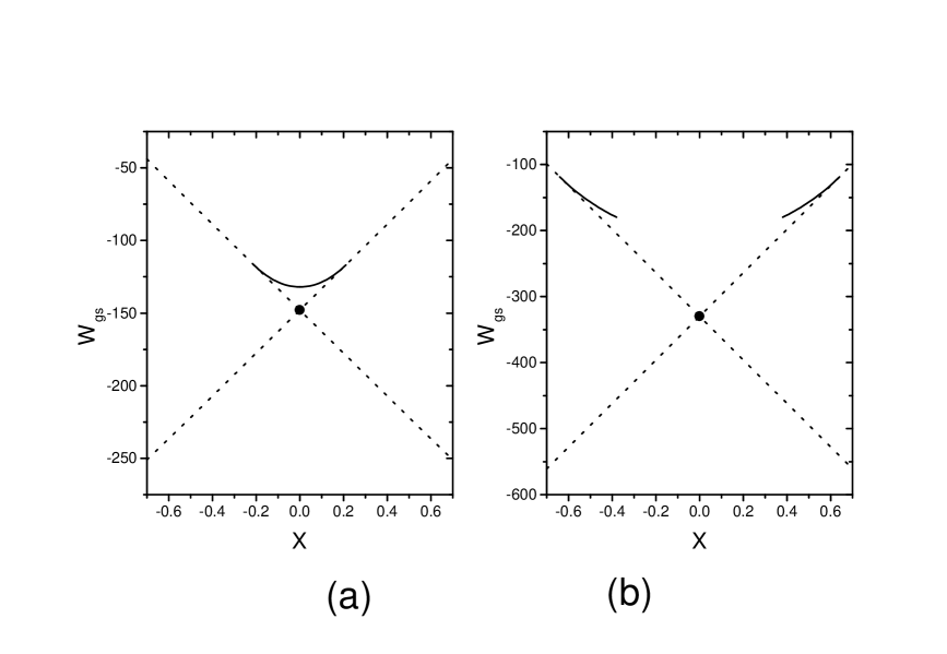
FIG. 1.: The vacuum energies $W_{gs}$ for a single $l$-shell as a function of $x$, (a) for $\eta=-0.80$ and (b) $\eta=-0.46$. Dotted lines: trivial solutions. Full: solution with $\Delta_{p}=\Delta_{n}$. Big dot: solution with $\Delta_{n}=-\Delta_{p}$.

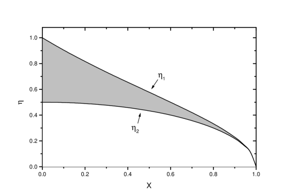
FIG. 2.: The allowed region in the $(x,\eta)$ plane for $\Delta_{n}=\Delta_{p}$.

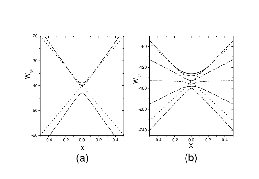
FIG. 3.: The energy spectrum as a function of $x$ for $\Omega=41$. (a) $A=4$ and (b) $A=16$. Dot-dashed lines: exact solutions. Dotted: trivial solutions. Full: solution with $\Delta_{n}=\Delta_{p}$.

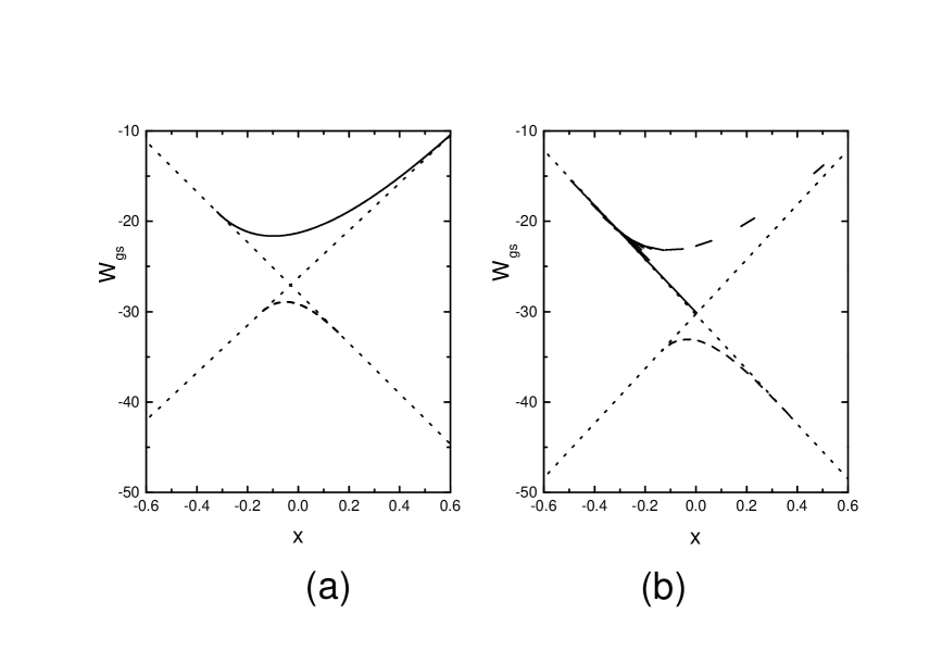
FIG. 4.: The vacuum energies $W_{gs}$ for a single $j$-shell as a function of $x$, for (a) $\eta=-4/11$ and (b) $\eta=0$. Dotted lines: trivial solutions. Dashed: solution with $\Delta_{n}=-\Delta_{p}$. Full: solution $\Delta_{n}=\Delta_{p}$.

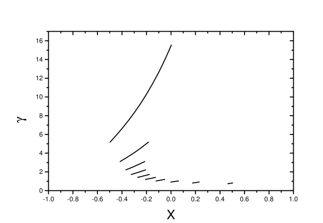
FIG. 5.: The asymmetry parameter $\gamma$ as a function of $x$, for $\eta=0$ (solution with $\Delta_{n}=\Delta_{p}$).

$\lambda$	$l$	$j$
$\mu$	$m,\sigma=\pm\frac{1}{2}$	$m$
$\mu>0$	$-l\leq m\leq l$, $\sigma=\frac{1}{2}$	$m>0$
$k_{\lambda\mu}$	$\frac{1}{\sqrt{2}}$	$m\sqrt{\frac{2}{j(j+1)}}$
$S^{{\dagger}}_{v}$	$-\sum_{l}\sqrt{\frac{2l+1}{2}}[c^{{\dagger}}_{l}c^{{\dagger}}_{l}]^{L=0,J=0,T=1}_{T_{0}=v}$	$-\sum_{j}\frac{\sqrt{2j+1}}{2}[c^{{\dagger}}_{j}c^{{\dagger}}_{j}]^{J=0,T=1}_{T_{0}=0}$
$S^{{\dagger}}_{0}$	$i\sum_{l}\sqrt{\frac{2l+1}{2}}[c^{{\dagger}}_{l}c^{{\dagger}}_{l}]^{L=0,J=1,T=0}_{J_{0}=0}$	$i\sum_{j}\sqrt{\frac{2j+1}{3}}[c^{{\dagger}}_{j}c^{{\dagger}}_{j}]^{J=1,T=0}_{J_{0}=0}$
$\eta$	$\frac{N_{p}}{2l+1}-1$	$\frac{N_{p}}{j+\frac{1}{2}}-1$

TABLE I.: The equivalence of the notation $\lambda,\mu$ in the $ls$ and $jj$ coupling schemes, the definition of the pairing operators $S_{v,0}^{{\dagger}}$ and of the occupation number $\eta$ ($-1\leq\eta\leq 1$).

$\Delta_{p}$	$\frac{1}{2}g_{1}(2l+1)\sqrt{1-\eta^{2}}$	0
$\Delta_{0}$	0	$\frac{1}{\sqrt{2}}g_{0}(2l+1)\sqrt{1-\eta^{2}}$
$\epsilon$	$-\eta E$	$-\eta E$
$E=E_{p}=E_{n}$	$\frac{1}{2}g_{1}(2l+1)$	$\frac{1}{2}g_{0}(2l+1)$
$W_{gs}$	$-\frac{1}{2}g_{1}(2l+1)^{2}(1-\eta^{2})$	$-\frac{1}{2}g_{0}(2l+1)^{2}(1-\eta^{2})$

TABLE II.: The solutions with $\Delta_{0}=0$ (second column) and $\Delta_{p}=0$ (third column) for a single $l$-shell.

	$1>\gamma m\sqrt{\frac{2}{j(j+1)}}$	$1<\gamma m\sqrt{\frac{2}{j(j+1)}}$
$\frac{1}{E_{p}}+\frac{1}{E_{n}}$	$2/\Delta_{p}(1-\frac{2m^{2}\gamma^{2}}{j(j+1)})$	$-2\gamma m\sqrt{\frac{2}{j(j+1)}}/\Delta_{p}(1-\frac{2m^{2}\gamma^{2}}{j(j+1)})$
$\frac{1}{E_{p}}-\frac{1}{E_{n}}$	$-2\gamma m\sqrt{\frac{2}{j(j+1)}}/\Delta_{p}(1-\frac{2m^{2}\gamma^{2}}{j(j+1)})$	$2/\Delta_{p}(1-\frac{2m^{2}\gamma^{2}}{j(j+1)})$
$y_{m}$	1	0

TABLE III.: The values of $\frac{1}{E_{p}}\pm\frac{1}{E_{n}}$ and of $y_{m}$ as functions of $\gamma$

$\gamma$	$y_{m}$	$\sum_{m>0}y_{m}$	$\sum_{m>0}my_{m}$	$x$
$\sqrt{2j(j+1)}<\gamma<\infty$	0	0	0	-1
$0<\gamma<\sqrt{\frac{j+1}{2j}}$	1	$j+\frac{1}{2}$	$\frac{1}{2}(j+\frac{1}{2})^{2}$	1

TABLE IV.: The behavior of the solution for very large and very small values of $\gamma$

REFERENCES

- [1] A. L. Goodman, Phys. Rev. C (in press).
- [2] S. Szpikowski, preprint ECT∗-97-008.
- [3] A. L. Goodman, Nucl. Phys. A186 475 (1972) and Advances in Nuclear Physics, edited by J. Negele and E. Vogt (Plenum, New York, 1979), Vol. 11, Chap. 4.11.
- [4] J. Dobeš and S. Pittel, Phys. Rev. C 57 688 (1998).
- [5] D. R. Bes and J. Kurchan, The Treatment of Collective Coordinates in Many-Body Systems (World Scientific, Singapore, 1990).
- [6] J. N. Ginocchio and J. Weneser, Phys. Rev. 170 859 (1968).
- [7] G. G. Dussel, R. P. J. Perazzo, D. R. Bes, and R. A. Broglia, Nucl. Phys. A 175 513 (1971).
- [8] J. Engel, K. Langanke, and P. Vogel, Phys. Lett. B 389 211 (1996).
- [9] J. Engel, S. Pittel, M. Stoitsov, P. Vogel, and J. Dukelsky, Phys. Rev. C 55 1781 (1997).
- [10] D. R. Bes, O. Civitarese, and N. N. Scoccola, Phys. Lett. B 446 93 (1999).
- [11] S. C. Pang, Nucl. Phys. A128 497 (1969).
- [12] J. A. Evans, G. G. Dussel, E.E. Maqueda, and R. P. J. Perazzo, Nucl. Phys. A367 77 (1981).