MKPH-T-99-16
Invariant amplitudes for coherent electromagnetic pseudoscalar production from a spin-one target (II): crossing, multipoles and observables

Abstract

The formal properties of the recently derived set of linearly independent invariant amplitudes for the electromagnetic production of a pseudoscalar particle from a spin-one particle have been further exploited. The crossing properties are discussed in detail. Since not all of the amplitudes have simple crossing behaviour, we introduce an alternative set of basic amplitudes which are either symmetric or antisymmetric under crossing. The multipole decomposition is given, and the representation of the multipoles as integrals over the invariant functions weighted with Legendre polynomials is derived. Furthermore, differential cross section and polarization observables are expressed in terms of the corresponding invariant functions.

I Introduction

Recently we have derived a set of 13 linearly independent invariant amplitudes for the electromagnetic production of a pseudoscalar particle from a spin-one particle in [1]. These amplitudes respect Lorentz and gauge invariance and the $T$-matrix can be represented by a linear superposition of them with invariant functions as coefficients, which depend on the Mandelstam variables only. Nine of these amplitudes are purely transverse and describe photoproduction while the remaining four appear in electroproduction in addition, describing charge and longitudinal current contributions.

In the present work we want to elaborate this formalism in further detail by exploring, for example, the crossing properties of the amplitudes and corresponding invariant functions and deriving explicit expressions for the observables. To this end, we first review briefly in Sect. II the set of basic amplitudes and discuss then in Sect. III their crossing properties. In view of the fact that not all 13 basic amplitudes introduced in [1] have simple crossing properties, we propose another alternative set of amplitudes which are either symmetric or antisymmetric under crossing. As next the multipole decomposition of the $T$-matrix will be discussed in Sect. IV where we give explicit expressions of the multipoles as integrals over the invariant functions weighted with linear combinations of Legendre polynomials. Then, in Sect. V we will define the various observables, i.e., differential cross section, beam and target asymmetries and the final state polarization observables. They are represented by structure functions which can be expressed in terms of the invariant functions.

II Brief review of the invariant amplitudes

As in [1], we consider as basic reaction the coherent pseudoscalar production by photoabsorption or electron scattering from a spin-one target

$$\gamma^{(*)}(k)+D(p)\rightarrow D(p^{\prime})+\Pi(q)\,,$$ (1)

where the real or virtual photon has momentum $k$ and polarization vector $\epsilon$, $D$ is a spin-one particle of mass $M$, henceforth called $D$ for brevity, with initial and final momenta $p$ and $p^{\prime}$ and $(S=1)$-spinors $U(\vec{p},m)$ and $U(\vec{p}^{\,\prime},m^{\prime})$, respectively, and $\Pi$ a pseudoscalar meson of mass $m$, henceforth called $\Pi$, with momentum $q$ (see Fig. 1).

As a first step we had derived in [1] using the principles of Lorentz covariance and parity conservation a set of basic amplitudes for the representation of the invariant reaction matrix element ${\cal M}_{fi}$. They are listed in Table I, where we use as a shorthand $U^{\prime}$ for $U^{\dagger}(\vec{p}^{\,\prime},m^{\prime})$ and $U$ for $U(\vec{p},m)$. Furthermore, we have introduced for convenience a covariant pseudoscalar by contraction of the four-dimensional Levi-Civita tensor $\varepsilon^{\mu\nu\rho\sigma}$ with four Lorentz vectors $a,\,b,\,c$ and $d$

$$S(a,b,c,d)=\varepsilon^{\mu\nu\rho\sigma}a_{\mu}b_{\nu}c_{\rho}d_{\sigma}\,.$$ (2)

Requiring in addition gauge invariance we were led to a restricted set of 13 gauge invariant amplitudes which are listed in Table II. Then the invariant matrix element can be represented as a linear superposition of this set of basic amplitudes, i.e.,

$${\cal M}_{fi}=\sum_{\alpha=1}^{13}F_{\alpha}(s,t,u)\,\Omega_{\alpha}\,,$$ (3)

where $F_{\alpha}(s,t,u)$ denote invariant functions which depend solely on the Mandelstam variables $s$, $t$ and $u$, defined as usual by

$$s=(k+p)^{2}\,,\quad t=(k-q)^{2}\,,\quad u=(k-p^{\prime}\,)^{2}\,,$$ (4)

of which only two are independent, for example, $s$ and $t$. It is obvious that the specific form of the invariant functions $F_{\alpha}(s,t,u)$ will depend on the detailed dynamical properties of the target and the produced meson.

The first nine amplitudes of Table II are purely transverse in the c.m. frame of photon and target particle, and thus are well suited for describing photoproduction. However, the remaining four, which in addition are needed in electroproduction, contain besides charge and longitudinal current components also transverse current pieces. For this reason we had replaced in [1] the last four amplitudes of Table II by equivalent amplitudes $\widetilde{\Omega}_{\alpha}$ which are purely longitudinal in the c.m. frame. This could be achieved by using the following relations given in Eqs. (33) through (36) of [1] which we repeat here in a more compact form because there some closing brackets were missing and, more importantly, the term containing $\Omega_{e}$ should not have been present in Eq. (34),

$$k\cdot p\,\Omega_{f}(k,x)-k_{\mu}^{2}\,\Omega_{f}(p,x) = (k_{\mu}^{2}+k\cdot p)\,\Omega_{h}(k,x)-k_{\mu}^{2}\,\Omega_{h}(q,x)$$ (6)

$$-[k,p\,;k,q]\,\Omega_{b}(k,p,x)+[k,p\,;k,p]\,\Omega_{b}(k,q,x)\,,$$

$$k\cdot p\,\Omega_{g}(x,k)-k_{\mu}^{2}\,\Omega_{g}(x,p) = k\cdot p\,\Omega_{h}(x,k)-k_{\mu}^{2}\,\Omega_{h}(x,q)$$ (8)

$$+[k,p\,;k,q]\,\Omega_{c}(k,p,x)-[k,p\,;k,p]\,\Omega_{c}(k,q,x)\,,$$

where $x\in\{k,q\}$, and the symbol $[a,b\,;c,d]$ is defined by

$$[a,b\,;c,d]:=(a\cdot c)(b\cdot d)-(a\cdot d)(b\cdot c)\,.$$ (9)

Therefore, we had replaced the last four amplitudes of Table II by the equivalent ones ($\widetilde{\Omega}_{\alpha}$) as given on the left hand side of (6) and (8) to be used for the longitudinal contributions in electroproduction. They are related to the $\Omega_{\alpha}$ according to (6) and (8) by

$$\widetilde{\Omega}_{10/11} = (k_{\mu}^{2}+k\cdot p)\,\Omega_{2/3}-k_{\mu}^{2}\,\Omega_{4/5}-[k,p\,;k,q]\,\Omega_{6/7}+[k,p\,;k,p]\,\Omega_{10/11}\,,$$ (10)

$$\widetilde{\Omega}_{12/13} = k\cdot p\,\Omega_{2/4}+[k,p\,;k,q]\,\Omega_{8/9}-[k,p\,;k,p]\,\Omega_{12/13}\,.$$ (11)

Then the reaction amplitude of (3) becomes

$${\cal M}_{fi}=\sum_{\alpha=1}^{13}\widetilde{F}_{\alpha}(s,t,u)\,\widetilde{\Omega}_{\alpha}\,,$$ (12)

where $\widetilde{\Omega}_{\alpha}=\Omega_{\alpha}$ for $\alpha=1,\dots,9$, and for $\alpha=10,\dots,13$ they are listed in Table III. Furthermore, the associated new invariant functions $\widetilde{F}_{\alpha}(s,t,u)$ are related to the $F_{\alpha}(s,t,u)$ introduced previously by

$$\widetilde{F}_{1} = F_{1}\,,$$ (13)

$$\widetilde{F}_{2} = F_{2}-\frac{1}{[k,p\,;k,p]}\,((k_{\mu}^{2}+k\cdot p)F_{10}-k\cdot pF_{12})\,,$$ (14)

$$\widetilde{F}_{3} = F_{3}-\frac{k_{\mu}^{2}+k\cdot p}{[k,p\,;k,p]}\,F_{11}\,,$$ (15)

$$\widetilde{F}_{4} = F_{4}+\frac{1}{[k,p\,;k,p]}\,(k_{\mu}^{2}F_{10}+k\cdot pF_{13})\,,$$ (16)

$$\widetilde{F}_{5} = F_{5}+\frac{k_{\mu}^{2}}{[k,p\,;k,p]}\,F_{11}\,,$$ (17)

$$\widetilde{F}_{6/7} = F_{6/7}+\frac{[k,p\,;k,q]}{[k,p\,;k,p]}\,F_{10/11}\,,$$ (18)

$$\widetilde{F}_{8/9} = F_{8/9}+\frac{[k,p\,;k,q]}{[k,p\,;k,p]}\,F_{12/13}\,,$$ (19)

$$\widetilde{F}_{10/11} = \frac{1}{[k,p\,;k,p]}\,F_{10/11}\,,$$ (20)

$$\widetilde{F}_{12/13} = -\frac{1}{[k,p\,;k,p]}\,F_{12/13}\,.$$ (21)

In these relations, one has to express the various kinematic factors in terms of the Mandelstam variables by using

$$k\cdot p = \frac{1}{2}\,(s-M^{2}+K^{2})\,,$$ (22)

$$k\cdot q = \frac{1}{2}\,(m^{2}-K^{2}-t)\,,$$ (23)

$$p\cdot q = \frac{1}{2}\,(s+t-M^{2}+K^{2})\,,$$ (24)

with $K^{2}=-k_{\mu}^{2}$. Since $[k,p\,;k,p]=-(K^{2}M^{2}+(k\cdot p)^{2})<0$, no kinematic singularities are introduced by these transformations.

For the study of the crossing properties of the $\widetilde{F}_{\alpha}$, the following inverse relations are useful

$$F_{2} = \widetilde{F}_{2}+(k_{\mu}^{2}+k\cdot p)\widetilde{F}_{10}+k\cdot p\widetilde{F}_{12}\,,$$ (25)

$$F_{3} = \widetilde{F}_{3}+(k_{\mu}^{2}+k\cdot p)\widetilde{F}_{11}\,,$$ (26)

$$F_{4} = \widetilde{F}_{4}+k_{\mu}^{2}\widetilde{F}_{10}-k\cdot p\widetilde{F}_{13}\,,$$ (27)

$$F_{5} = \widetilde{F}_{5}-k_{\mu}^{2}\widetilde{F}_{11}\,,$$ (28)

$$F_{6/7} = \widetilde{F}_{6/7}-[k,p\,;k,q]\,\widetilde{F}_{10/11}\,,$$ (29)

$$F_{8/9} = \widetilde{F}_{8/9}+[k,p\,;k,q]\,\widetilde{F}_{12/13}\,,$$ (30)

$$F_{10/11} = [k,p\,;k,p]\widetilde{F}_{10/11}\,,$$ (31)

$$F_{12/13} = -[k,p\,;k,p]\widetilde{F}_{12/13}\,.$$ (32)

Although these new amplitudes allow a clear separation of the invariant functions into longitudinal and transverse contributions, they also carry a disadvantage, namely a much more complicated crossing behaviour as is discussed in the next section.

III Crossing properties

Now we will study the crossing properties of the invariant functions with respect to the interchange of the initial with the final spin-one particle. To this end we will study the general structure of the reaction matrix shown in Fig. 1 for the $s$- and $u$-channels in analogy to electromagnetic pion production on the nucleon [2]. The reaction matrix is governed by the current operator

$$j^{\nu}_{\gamma D\,\Pi}(x)=\Phi^{\dagger}_{D,\,\mu}(x)\,J^{\mu\nu\rho}(x)\,\Phi_{D,\,\rho}(x)\,\Phi_{\Pi}(x)\,.$$ (33)

Here, $\Phi_{\Pi}(x)$ represents the usual field operator of a neutral pseudoscalar field and $\Phi^{\mu}_{D}(x)$ the one of a charged, massive vector field

$$\Phi^{\mu}_{D}(x)=N_{\pi}\,\sum_{\lambda}\int\frac{d^{3}p}{2\omega_{p}}\,\Big{(}U^{\mu}(\vec{p},\lambda)\,A_{D}(\vec{p},\lambda)e^{-ip\cdot x}+U^{\mu\ast}(\vec{p},\lambda)\,B_{\bar{D}}^{\dagger}(\vec{p},\lambda)e^{ip\cdot x}\Big{)}\,,$$ (34)

where $N_{\pi}$ is a normalization constant, $U^{\mu}(\vec{p},\lambda)$ a polarization vector, $A_{D}(\vec{p},\lambda)$ the anihilation operator of a $D$-particle with momentum $\vec{p}$ and helicity $\lambda$, and $B_{\bar{D}}^{\dagger}(\vec{p},\lambda)$ the creation operator of a corresponding antiparticle $\bar{D}$. These operators transform under charge conjugation

$$C\,A_{D}(\vec{p},\lambda)\,C^{-1} = B_{\bar{D}}(\vec{p},\lambda)\,,$$ (35)

$$C\,B_{\bar{D}}^{\dagger}(\vec{p},\lambda)\,C^{-1} = A_{D}^{\dagger}(\vec{p},\lambda)\,,$$ (36)

$$C\,U^{\mu}(\vec{p},\lambda)\,C^{-1} = U^{\mu T}(\vec{p},\lambda)\,.$$ (37)

For the $s$-channel, i.e., pseudoscalar production on $D$, one obtains for the current matrix element

$$\langle D(p^{\prime},\lambda^{\prime})\Pi(q)|\epsilon_{\nu}(k,\lambda_{\gamma})\, j^{\nu}_{\gamma D\,\Pi}(0)|D(p,\lambda)\gamma(k,\lambda_{\gamma})\rangle=$$ (39)

$$N_{\pi}^{3}\sum_{\alpha=1}^{13}F_{\alpha}(s,t,u)\,U_{\mu}^{\dagger}(\vec{p}^{\,\prime},\lambda^{\prime})\,\epsilon_{\nu}(k,\lambda_{\gamma})\,{\cal O}^{\mu\nu\rho}_{\alpha}(k,p,q)\,U_{\rho}(\vec{p},\lambda)\,.$$

Similarly, one finds for the $u$-channel, i.e., $\Pi$ production on a $\bar{D}$

$$\langle\bar{D}(-p,\lambda)\Pi(q)|\epsilon_{\nu}(k,\lambda_{\gamma}) \,j^{\nu}_{\gamma D\,\Pi}(0)|\bar{D}(-p^{\prime},\lambda^{\prime})\gamma(k,\lambda_{\gamma})\rangle=$$ (41)

$$N_{\pi}^{3}\sum_{\alpha=1}^{13}F_{\alpha}(s,t,u)\,U_{\mu}^{T}(-\vec{p}^{\,\prime},\lambda^{\prime})\,\epsilon_{\nu}(k,\lambda_{\gamma})\,{\cal O}^{\mu\nu\rho}_{\alpha}(k,p,q)\,U_{\rho}^{\ast}(-\vec{p},\lambda)\,.$$

Now using invariance under charge conjugation of $\epsilon_{\nu}j^{\nu}$ and the transformations

$$C|\gamma(k,\lambda_{\gamma})\rangle=-|\gamma(k,\lambda_{\gamma})\rangle\,,\quad C|D(p,\lambda)\rangle=|\bar{D}(p,\lambda)\rangle\,,\quad C|\Pi(q)\rangle=|\Pi(q)\rangle\,,$$ (42)

one finds

$$\langle D(p^{\prime},\lambda^{\prime})\Pi(q)|\epsilon_{\nu}(k,\lambda_{\gamma})\, j^{\nu}_{\gamma D\Pi}(0)|D(p,\lambda)\gamma(k,\lambda_{\gamma})\rangle=$$ (44)

$$-\langle\bar{D}(p^{\prime},\lambda^{\prime})\Pi(q)|\epsilon_{\nu}(k,\lambda_{\gamma})\,j^{\nu}_{\gamma D\Pi}(0)|\bar{D}(p,\lambda)\gamma(k,\lambda_{\gamma})\rangle\,.$$

Inserting the explicit expressions from (39) and (41), one obtains the general crossing relation

$$\sum_{\alpha=1}^{13}F_{\alpha}(s,t,u)\, U_{\mu}^{\dagger}(\vec{p}^{\,\prime},\lambda^{\prime})\,\epsilon_{\nu}(k,\lambda_{\gamma})\,{\cal O}^{\mu\nu\rho}_{\alpha}(k,p,q)\,U_{\rho}(p,\lambda)=$$ (46)

$$-\sum_{\alpha=1}^{13}F_{\alpha}(u,t,s)\,U_{\mu}^{T}(\vec{p},\lambda)\,\epsilon_{\nu}(k,\lambda_{\gamma})\,{\cal O}^{\mu\nu\rho}_{\alpha}(k,-p^{\prime},q)\,U_{\rho}^{\ast}(p^{\prime},\lambda^{\prime})\,.$$

Introducing the transformation of the basic amplitudes $\Omega_{\alpha}$ under crossing, i.e., $U^{\ast}(\vec{p}^{\,\prime},\lambda^{\prime})\leftrightarrow U(\vec{p},\lambda)$ and $p\leftrightarrow-p^{\prime}$ ($s\leftrightarrow u$), according to

$$\Omega_{\alpha}=U_{\mu}^{\dagger}(\vec{p}^{\,\prime},\lambda^{\prime})\,\epsilon_{\nu}O^{\mu\nu\rho}_{\alpha}(k,p,q)\,U_{\rho}(\vec{p},\lambda)$$ (47)

$$\stackrel{{\scriptstyle\mbox{{crossing}}}}{{\longrightarrow}}\quad\Omega_{\alpha}^{c} = U_{\mu}^{T}(\vec{p},\lambda)\,\epsilon_{\nu}O^{\mu\nu\rho}_{\alpha}(k,-p^{\prime},q)\,U_{\rho}^{\ast}(\vec{p}^{\,\prime},\lambda^{\prime})\,,$$ (48)

the general crossing relation of (46) then reads

$$\sum_{\alpha=1}^{13}F_{\alpha}(s,t,u)\,\Omega_{\alpha}\,=-\sum_{\alpha=1}^{13}F_{\alpha}(u,t,s)\,\Omega_{\alpha}^{c}\,.$$ (49)

From the explicit expressions of the basic amplitudes in Table I one finds easily the following crossing transformations

$$\Omega_{e}(\epsilon,U^{\prime},U) \rightarrow -\Omega_{e}(\epsilon,U^{\prime},U)\,,$$ (50)

$$\Omega_{h}(x,y) \rightarrow -\Omega_{h}(x,y)\,,$$ (51)

$$\Omega_{b/c}(k,p,x) \rightarrow \Omega_{c/b}(k,p,x)-\Omega_{c/b}(k,q,x)\,,$$ (52)

$$\Omega_{b/c}(k,q,x) \rightarrow -\Omega_{c/b}(k,q,x)\,,$$ (53)

for $x,y\in\{k,q\}$. This leads to the crossing transformations of the gauge invariant amplitudes of Table II

$$\Omega_{\alpha}^{c} = -\Omega_{\alpha}\,,\mbox{ for }\,\alpha=1,2,5\,,$$ (54)

$$\Omega_{3/4}^{c} = -\Omega_{4/3}\,,$$ (55)

$$\Omega_{6/7}^{c} = \Omega_{8/9}-\Omega_{12/13}\,,$$ (56)

$$\Omega_{8/9}^{c} = \Omega_{6/7}-\Omega_{10/11}\,,$$ (57)

$$\Omega_{10/11}^{c} = -\Omega_{12/13}\,,$$ (58)

$$\Omega_{12/13}^{c} = -\Omega_{10/11}\,.$$ (59)

Thus the crossing relation (49) requires the invariant functions $F_{\alpha}(s,t,u)$ to possess the following crossing properties

$$F_{\alpha}(s,t,u) = F_{\alpha}(u,t,s)\,,\mbox{ for }\,\alpha=1,2,5\,,$$ (60)

$$F_{3/4}(s,t,u) = F_{4/3}(u,t,s)\,,$$ (61)

$$F_{6/7}(s,t,u) = -F_{8/9}(u,t,s)\,,$$ (62)

$$F_{8/9}(s,t,u) = -F_{6/7}(u,t,s)\,,$$ (63)

$$F_{10/11}(s,t,u) = F_{8/9}(u,t,s)+F_{12/13}(u,t,s)\,,$$ (64)

$$F_{12/13}(s,t,u) = F_{6/7}(u,t,s)+F_{10/11}(u,t,s)\,.$$ (65)

For the alternative basic amplitudes $\widetilde{\Omega}_{\alpha}$ one finds for $\alpha=1,\dots,5$ the same crossing behaviour as for $\Omega_{\alpha}$ in (59). For the other amplitudes one has to eliminate from the above crossing transformations the amplitudes $\Omega_{10/\dots/13}$ by using (10) and (11) resulting in

$$\widetilde{\Omega}_{6/7}^{c} = \frac{1}{[k,p\,;k,p]}\,(-k\cdot p\widetilde{\Omega}_{2/4}+[k,p\,;k,p^{\prime}]\widetilde{\Omega}_{8/9}-\widetilde{\Omega}_{12/13})\,,$$ (66)

$$\widetilde{\Omega}_{8/9}^{c} = \frac{1}{[k,p\,;k,p]}\,((k_{\mu}^{2}+k\cdot p)\widetilde{\Omega}_{2/3}-k_{\mu}^{2}\,\widetilde{\Omega}_{4/5}+[k,p\,;k,p^{\prime}]\widetilde{\Omega}_{6/7}-\widetilde{\Omega}_{10/11})\,,$$ (67)

$$\widetilde{\Omega}_{10/11}^{c} = \frac{1}{[k,p\,;k,p]}\,(-k_{\mu}^{2}\,[k,p\,;q,p]\widetilde{\Omega}_{2/4}+k_{\mu}^{2}\,[k,p\,;k,p]\widetilde{\Omega}_{3/5}$$ (69)

$$\hskip 42.67912pt+((k\cdot p)^{2}-(k\cdot p^{\prime})^{2})[k,p^{\prime}\,;k,p^{\prime}]\widetilde{\Omega}_{8/9}+[k,p^{\prime}\,;k,p]\widetilde{\Omega}_{12/13})\,,$$

$$\widetilde{\Omega}_{12/13}^{c} = \frac{1}{[k,p\,;k,p]}\,(k_{\mu}^{2}\,[k,p\,;(k+p),q]\widetilde{\Omega}_{2/3}+k_{\mu}^{2}\,[k,p^{\prime}\,;k,p]\widetilde{\Omega}_{4/5}$$ (71)

$$\hskip 42.67912pt-((k\cdot p)^{2}-(k\cdot p^{\prime})^{2})[k,p^{\prime}\,;k,p^{\prime}]\widetilde{\Omega}_{6/7}+[k,p^{\prime}\,;k,p]\widetilde{\Omega}_{10/11})\,.$$

Correspondingly, the crossing properties of the invariant functions $\widetilde{F}_{\alpha}(s,t,u)$ are more involved. Explicitly one finds using either (71) or (65) in conjunction with (21) and (32)

$$\widetilde{F}_{1}(s,t,u) = \widetilde{F}_{1}(u,t,s)\,,$$ (72)

$$\widetilde{F}_{2}(s,t,u) = \widetilde{F}_{2}(u,t,s)+\frac{1}{[k,p\,;k,p]}(k\cdot p\,\widetilde{F}_{6}(u,t,s)-(k_{\mu}^{2}+k\cdot p)\,\widetilde{F}_{8}(u,t,s)$$ (74)

$$+k_{\mu}^{2}\,[k,p\,;q,p]\,\widetilde{F}_{10}(u,t,s)-k_{\mu}^{2}\,[k,p\,;(k+p),q]\,\widetilde{F}_{12}(u,t,s))\,,$$

$$\widetilde{F}_{3}(s,t,u) = \widetilde{F}_{4}(u,t,s)-\frac{1}{[k,p\,;k,p]}((k_{\mu}^{2}+k\cdot p)\,\widetilde{F}_{9}(u,t,s)$$ (76)

$$+k_{\mu}^{2}\,[k,p\,;k,p]\,\widetilde{F}_{10}(u,t,s)+k_{\mu}^{2}\,[k,p\,;(k+p),q]\,\widetilde{F}_{13}(u,t,s))\,,$$

$$\widetilde{F}_{4}(s,t,u) = \widetilde{F}_{3}(u,t,s)+\frac{1}{[k,p\,;k,p]}(k\cdot p\,\widetilde{F}_{7}(u,t,s)+k_{\mu}^{2}\,\widetilde{F}_{8}(u,t,s)$$ (78)

$$+k_{\mu}^{2}\,[k,p\,;q,p]\,\widetilde{F}_{11}(u,t,s)-k_{\mu}^{2}\,[k,p^{\prime}\,;k,p]\,\widetilde{F}_{12}(u,t,s))\,,$$

$$\widetilde{F}_{5}(s,t,u) = \widetilde{F}_{5}(u,t,s)-\frac{1}{[k,p\,;k,p]}(k_{\mu}^{2}\,\widetilde{F}_{9}(u,t,s)$$ (80)

$$-k_{\mu}^{2}\,[k,p\,;k,p]\,\widetilde{F}_{11}(u,t,s)-k_{\mu}^{2}\,[k,p^{\prime}\,;k,p]\,\widetilde{F}_{13}(u,t,s))\,,$$

$$\widetilde{F}_{6/7}(s,t,u) = \frac{1}{[k,p\,;k,p]}(-[k,p^{\prime}\,;k,p]\,\widetilde{F}_{8/9}(u,t,s)$$ (82)

$$+((k\cdot p)^{2}-(k\cdot p^{\prime})^{2})\,[k,p^{\prime}\,;k,p^{\prime}]\,\widetilde{F}_{12/13}(u,t,s))\,,$$

$$\widetilde{F}_{8/9}(s,t,u) = \frac{1}{[k,p\,;k,p]}(-[k,p^{\prime}\,;k,p]\,\widetilde{F}_{6/7}(u,t,s)$$ (84)

$$-((k\cdot p)^{2}-(k\cdot p^{\prime})^{2})\,[k,p^{\prime}\,;k,p^{\prime}]\,\widetilde{F}_{10/11}(u,t,s))\,,$$

$$\widetilde{F}_{10/11}(s,t,u) = \frac{1}{[k,p\,;k,p]}(\widetilde{F}_{8/9}(u,t,s)-[k,p^{\prime}\,;k,p^{\prime}]\,\widetilde{F}_{12/13}(u,t,s))\,,$$ (85)

$$\widetilde{F}_{12/13}(s,t,u) = \frac{1}{[k,p\,;k,p]}(\widetilde{F}_{6/7}(u,t,s)-[k,p^{\prime}\,;k,p^{\prime}]\,\widetilde{F}_{10/11}(u,t,s))\,.$$ (86)

If one wants simpler crossing properties of the basic amplitudes and invariant functions, one can introduce another alternative set of gauge invariant amplitudes $\widehat{\Omega}_{\alpha}$ by taking appropriate linear combinations of the original $\Omega_{\alpha}$

$$\widehat{\Omega}_{\alpha} = \Omega_{\alpha}\,,\mbox{ for }\,\alpha=1,2,5\,,$$ (87)

$$\widehat{\Omega}_{3/4} = \Omega_{3}\pm\Omega_{4}\,,$$ (88)

$$\widehat{\Omega}_{6/8} = \Omega_{6}\pm\Omega_{8}-\frac{1}{2}\widehat{\Omega}_{10/12}\,,$$ (89)

$$\widehat{\Omega}_{7/9} = \Omega_{7}\pm\Omega_{9}-\frac{1}{2}\widehat{\Omega}_{11/13}\,,$$ (90)

$$\widehat{\Omega}_{10/12} = \Omega_{10}\pm\Omega_{12}\,,$$ (91)

$$\widehat{\Omega}_{11/13} = \Omega_{11}\pm\Omega_{13}\,.$$ (92)

The explicit forms of those which are different from $\Omega_{\alpha}$ are listed in Table IV where we have introduced in addition to the shorthand $[a,b\,;c,d]$ defined in (9)

$$\{a,b\,;c,d\} := (a\cdot c)(b\cdot d)+(a\cdot d)(b\cdot c)\,,$$ (93)

$$\widehat{S}^{\mu}(x) := \varepsilon^{\mu\nu\rho\sigma}\epsilon_{\nu}k_{\rho}x_{\sigma}\,.$$ (94)

Then one may represent the invariant matrix element ${\cal M}_{fi}$ in terms of these new amplitudes introducing appropriate new invariant functions $\widehat{F}_{\alpha}(s,t,u)$ by

$${\cal M}_{fi}=\sum_{\alpha=1}^{13}\widehat{F}_{\alpha}(s,t,u)\,\widehat{\Omega}_{\alpha}\,.$$ (95)

The $\widehat{F}_{\alpha}$ are related to the original invariant functions $F_{\alpha}$ by

$$\widehat{F}_{\alpha} = F_{\alpha},\mbox{ for }\,\alpha=1,2,5\,,$$ (96)

$$\widehat{F}_{3/4} = \frac{1}{2}\,(F_{3}\pm F_{4})\,,$$ (97)

$$\widehat{F}_{6/8} = \frac{1}{2}\,(F_{6}\pm F_{8})\,,$$ (98)

$$\widehat{F}_{7/9} = \frac{1}{2}\,(F_{7}\pm F_{9})\,,$$ (99)

$$\widehat{F}_{10/12} = \frac{1}{2}\,(F_{10}\pm F_{12}+\frac{1}{2}\,(F_{6}\pm F_{8}))\,,$$ (100)

$$\widehat{F}_{11/13} = \frac{1}{2}\,(F_{11}\pm F_{13}+\frac{1}{2}\,(F_{7}\pm F_{9}))\,.$$ (101)

The new amplitudes $\widehat{\Omega}_{\alpha}$ now have very simple crossing properties, namely

$$\widehat{\Omega}_{\alpha}^{c}=\left\{\begin{array}[]{rl}\widehat{\Omega}_{\alpha},&\mbox{ for }\,\alpha=1,2,3,5,8,9,10,11,\\ -\widehat{\Omega}_{\alpha},&\mbox{ for }\,\alpha=4,6,7,12,13,\end{array}\right.$$ (102)

from which follows a correspondingly simple crossing behaviour of the $\widehat{F}_{\alpha}$

$$\widehat{F}_{\alpha}(s,t,u)=\left\{\begin{array}[]{rl}\widehat{F}_{\alpha}(u,t,s),&\mbox{ for }\,\alpha=4,6,7,12,13,\\ -\widehat{F}_{\alpha}(u,t,s),&\mbox{ for }\,\alpha=1,2,3,5,8,9,10,11.\end{array}\right.$$ (103)

However, one has to keep in mind that these new amplitudes do not separate into transverse and longitudinal ones.

IV Multipole decomposition

As in [1], we choose as basic reference frame one which has its $z$-axis parallel to the incoming real or virtual photon. For real photons the $x$-axis is chosen in the direction of maximal linear polarization, whereas for virtual photons the $y$-axis is taken perpendicular to the electron scattering plane, i.e., parallel to $\vec{k}_{1}^{lab}\times\vec{k}_{2}^{lab}$ where $k_{1}^{lab}$ and $k_{2}^{lab}$ denote the lab frame momenta of the initial and the scattered electrons, respectively. The final state is described by the angles $\theta$ and $\phi$ of the momentum $\vec{q}$ with respect to the basic frame of reference.

Taking the representation of the $(S=1)$-spinors as given in (37) and (38) of [1], the helicity representation of the invariant amplitude can be written in the form

$$T_{\lambda^{\prime}\lambda_{\gamma}\lambda}(\theta,\phi) = e^{i(\lambda_{\gamma}-\lambda)\phi}t_{\lambda^{\prime}\lambda_{\gamma}\lambda}(\theta)$$ (104)

with

$$t_{\lambda^{\prime}\lambda_{\gamma}\lambda}(\theta) = \sum_{\alpha}\widetilde{F}_{\alpha}(s,t,u)\,\widetilde{\Omega}_{\alpha,\lambda^{\prime}\lambda_{\gamma}\lambda}(\theta)\,,$$ (105)

thus separating the $\phi$-dependence. Here, $\widetilde{F}_{\alpha}$ and $\widetilde{\Omega}_{\alpha}$ may be replaced by $F_{\alpha}$ and $\Omega_{\alpha}$ or $\widehat{F}_{\alpha}$ and $\widehat{\Omega}_{\alpha}$ depending on the choice of basic amplitudes. Explicit expressions of the helicity matrix elements of the various invariant amplitudes $\widetilde{\Omega}_{\alpha}$ are listed in Table 5 of [1]. Note that in [1] we had chosen $\phi=0$.

The reduced matrix element $t_{\lambda^{\prime}\lambda_{\gamma}\lambda}(\theta)$ will now be expanded into charge or longitudinal, electric and magnetic multipoles. For the definition of the multipole decomposition we extend the convention of [3] for real photons to virtual ones including charge multipoles as follows

$$t_{\lambda^{\prime}\lambda_{\gamma}\lambda}(\theta) = \sqrt{\frac{1+\delta_{\lambda_{\gamma}0}}{2}}\sum_{L}\sum_{lj}\frac{\hat{L}\hat{l}}{\hat{\jmath}}(l01-\lambda^{\prime}|j-\lambda^{\prime})(1-\lambda L\lambda_{\gamma}|j\,\lambda_{\gamma}-\lambda)\,O^{L\lambda_{\gamma}}_{lj}d^{j}_{\lambda_{\gamma}-\lambda,-\lambda^{\prime}}(\theta)\,,$$ (106)

where $\hat{\jmath}=\sqrt{2j+1}$, and $(j_{1}m_{1}j_{2}m_{2}|jm)$ denotes a Clebsch-Gordan coefficient. Here $j$ and $l$ denote total and orbital angular momentum, respectively, of a final state partial wave, and $L$ the e.m. multipolarity. Furthermore, $O^{L\lambda_{\gamma}}_{lj}$ contains the electric $(E^{L}_{lj})$, magnetic $(M^{L}_{lj})$ and coulomb or longitudinal $(C^{L}_{lj})$ multipoles according to

$$O^{L\lambda_{\gamma}}_{lj}=\delta_{|\lambda_{\gamma}|,1}(E^{L}_{lj}+\lambda_{\gamma}M^{L}_{lj})+\delta_{\lambda_{\gamma},0}C^{L}_{lj}\,.$$ (107)

Thus the various multipole types are obtained from $O^{L\lambda_{\gamma}}_{lj}$ by

$$C^{L}_{lj} = O^{L0}_{lj}\,,$$ (108)

$$(E/M)^{L}_{lj} = \frac{1}{2}(O^{L1}_{lj}\pm O^{L-1}_{lj})\,.$$ (109)

Using the orthogonality properties of the $d^{j}$-matrices [4], one finds

$$O^{L\lambda_{\gamma}}_{lj} = \frac{\hat{\jmath}}{\sqrt{2(1+\delta_{\lambda_{\gamma}0})}}\sum_{\lambda^{\prime}\lambda}\,C^{1lj}_{-\lambda^{\prime},0,\lambda^{\prime}}\,C^{1Lj}_{\lambda,-\lambda_{\gamma},\lambda_{\gamma}-\lambda}\,\int_{-1}^{1}d(\cos\theta)\,t_{\lambda^{\prime}\lambda_{\gamma}\lambda}(\theta)\,d^{j}_{\lambda-\lambda_{\gamma},\lambda^{\prime}}(\theta)\,.$$ (110)

where we have defined

$$C^{j_{1}j_{2}j_{3}}_{m_{1},m_{2},m_{3}}=\left(\matrix{j_{1}&j_{2}&j_{3}\cr m_{1}&m_{2}&m_{3}\cr}\right)\,$$ (111)

as a shorthand for a $3j$-symbol. From (108) and (109) one obtains in detail

$$C^{L}_{lj} = \frac{\hat{\jmath}}{2}\sum_{\lambda^{\prime}\lambda}C^{1lj}_{-\lambda^{\prime},0,\lambda^{\prime}}\,C^{1Lj}_{\lambda,0,-\lambda}\,\int_{-1}^{1}d(\cos\theta)\,t_{\lambda^{\prime}0\lambda}(\theta)\,d^{j}_{\lambda,\lambda^{\prime}}(\theta)\,,$$ (112)

$$(E/M)^{L}_{lj} = \frac{1}{2}\,(1\mp(-)^{l+L})\,\frac{\hat{\jmath}}{\sqrt{2}}\,\sum_{\lambda^{\prime}\lambda}\,C^{1lj}_{-\lambda^{\prime},0,\lambda^{\prime}}\,C^{1Lj}_{\lambda,-1,1-\lambda}\,\int_{-1}^{1}d(\cos\theta)\,t_{\lambda^{\prime}1\lambda}(\theta)\,d^{j}_{\lambda-1,\lambda^{\prime}}(\theta)\,,$$ (113)

where in the latter case use has been made of the parity property

$$t_{-\lambda^{\prime}-\lambda_{\gamma}-\lambda}=(-)^{1+\lambda^{\prime}+\lambda_{\gamma}+\lambda}t_{\lambda^{\prime}\lambda_{\gamma}\lambda}\,.$$ (114)

The resulting multipole transitions, which can reach a given partial wave $(l,j)$, are listed in Table V.

For the explicit representation of the multipoles one has to introduce the expansion of the reduced $t$-matrix into invariant amplitudes from (105). Factorizing the helicity representation of the invariant amplitudes in a helicity independent part $\widetilde{\rho}^{\,\alpha}$ and a helicity dependent part $\widetilde{\omega}^{\,\alpha}_{\lambda^{\prime}\lambda_{\gamma}\lambda}$ as listed in Table VI by

$$\widetilde{\Omega}_{\alpha,\,\lambda^{\prime}\lambda_{\gamma}\lambda}(\theta)=\widetilde{\rho}^{\,\alpha}\,\widetilde{\omega}^{\,\alpha}_{\lambda^{\prime}\lambda_{\gamma}\lambda}(\theta)\,,$$ (115)

and introducing

$$o^{(lj)L\lambda_{\gamma}}_{\alpha}(\theta)=\sum_{\lambda^{\prime}\lambda}C^{1lj}_{-\lambda^{\prime},0,\lambda^{\prime}}C^{1Lj}_{\lambda,-\lambda_{\gamma},\lambda_{\gamma}-\lambda}\,\widetilde{\omega}^{\,\alpha}_{\lambda^{\prime}\lambda_{\gamma}\lambda}(\theta)\,d^{j}_{\lambda-\lambda_{\gamma},\lambda^{\prime}}(\theta)\,,$$ (116)

one finds for the multipoles the compact form

$$O^{L\lambda_{\gamma}}_{lj}=\frac{\hat{\jmath}}{\sqrt{2(1+\delta_{\lambda_{\gamma}0})}}\sum_{\alpha}\widetilde{\rho}^{\,\alpha}\,\int_{-1}^{1}d(\cos\theta)\,\widetilde{F}_{\alpha}(s,t,u)\,o^{(lj)L\lambda_{\gamma}}_{\alpha}(\theta)\,,$$ (117)

where for $|\lambda_{\gamma}|=1$ the sum over $\alpha$ runs from 1 through 9 and for $\lambda_{\gamma}=0$ from 10 through 13. The evaluation of the $o^{(lj)L\lambda_{\gamma}}_{\alpha}(\theta)$ is straightforward although somewhat lengthy. With the help of the addition theorem of the $d^{j}$-matrices [4], one can expand the $o^{(lj)L\lambda_{\gamma}}_{\alpha}(\theta)$ in terms of Legendre polynomials. Explicit expressions are given in the Appendix A.

V Differential cross section and polarization observables

For the representation of observables we will take the same formal framework than used in deuteron photo- and electrodisintegration following the treatment in [5, 6, 7]. Any observable in coherent scalar or pseudoscalar photo- or electroproduction off a spin-one target may be given in the form

$${\cal O}_{X}=3c\,\mbox{Tr}\,(T^{\dagger}\widehat{O}_{X}T\rho)\,,$$ (118)

where the trace refers to the spin degrees of freedom of initial and final states, and $c$ is a kinematic factor explained below. Here $X$ characterizes an observable associated with the analysis of the final target spin state. We choose the representation $X=(IM\pm)$ $(I=0,1,2;\,I\geq M\geq 0)$ with a corresponding hermitean operator

$$\widehat{O}_{IM{\rm sig}_{M}}=c_{M{\rm sig}_{M}}(\tau^{[I]}_{M}+{\rm sig}_{M}(-)^{M}\tau^{[I]}_{-M})\,,$$ (119)

with

$$c_{M{\rm sig}_{M}}=\left\{\matrix{\frac{1}{1+\delta_{M0}},&\mbox{ for }\,{\rm sig}_{M}=+\,,\cr i,&\mbox{ for }\,{\rm sig}_{M}=-\,.\cr}\right.$$ (120)

Here we have introduced a sign function by ${\rm sig}_{M}:=\pm$, where the subscript $M$ merely indicates to which variable it refers.

The irreducible tensors $\tau^{[I]}$ are the usual statistical tensors for the parametrization of the density matrix of a spin-one particle with normalization $\langle 1||\tau^{[I]}||1\rangle=\sqrt{3}\,\hat{I}$, i.e. in detail

$$\tau^{[I]}=\left\{\begin{array}[]{cl}{\mathbb{1}}_{3}&\mbox{ no polarization,}\\ \sqrt{\frac{3}{2}}\,S^{[1]}&\mbox{ vector polarization,}\\ \sqrt{3}\,S^{[2]}&\mbox{ tensor polarization,}\end{array}\right.$$ (121)

where ${\mathbb{1}}_{3}$ is the unit matrix, $S^{[1]}$ the spin operator, and $S^{[2]}=[S^{[1]}\times S^{[1]}]^{[2]}$ the tensor operator of a spin-one particle. In particular, we note the property

$$(\tau^{[I]}_{M})^{\dagger}=(-)^{M}\,\tau^{[I]}_{-M}\,.$$ (122)

Furthermore, the initial state density matrix $\rho$ is composed from the density matrices of the photon $\rho^{\gamma}$ and the one of the spin-one particle $\rho^{D}$

$$\rho=\rho^{\gamma}\otimes\rho^{D}\,.$$ (123)

For virtual photons, i.e., electron scattering, the kinematic factor $c$ reads

$$c(k_{1}^{lab},k^{lab}_{2})={\alpha\over 6\pi^{2}}{k^{lab}_{2}\over k_{1}^{lab}q_{\nu}^{4}}\;,$$ (124)

where $\alpha$ is the fine structure constant and $q_{\nu}^{2}=q_{0}^{2}-\vec{q}^{\,2}$ denotes the four momentum transfer squared $(q=k_{1}-k_{2})$. In this case the density matrix is given by

$$\rho^{\gamma^{*}}_{\lambda_{\gamma}\lambda_{\gamma}^{\prime}}=\sum_{\alpha=\{L,T,LT,TT\}}(\delta^{\alpha}_{\lambda_{\gamma}\lambda_{\gamma}^{\prime}}\rho_{\alpha}+h\delta^{\prime\alpha}_{\lambda_{\gamma}\lambda_{\gamma}^{\prime}}\rho_{\alpha}^{\prime})\,,$$ (125)

where

$$\rho_{L}=-\beta^{2}q^{2}_{\nu}{\xi^{2}\over 2\eta}\,,\hskip 25.6073pt \hskip 28.45274pt\rho_{LT}=-\beta q^{2}_{\nu}{\xi\over\eta}\sqrt{{\xi+\eta\over 8}}\;,$$ (126)

$$\rho_{T}=-{1\over 2}q^{2}_{\nu}(1+{\xi\over 2\eta})\,, \hskip 28.45274pt\rho_{TT}=q^{2}_{\nu}{\xi\over 4\eta}\;,$$ (127)

$$\rho^{\prime}_{T}=-{1\over 2}q^{2}_{\nu}\sqrt{{\xi+\eta\over\eta}}\,,\,\,\,\, \hskip 28.45274pt\rho^{\prime}_{LT}=-{1\over 2}\beta q^{2}_{\nu}{\xi\over\sqrt{2\eta}}\;,$$ (128)

with

$$\beta={|{\vec{q}}^{\,lab}|\over|{\vec{q}}^{\,c}|},\,\,\,\,\,\xi=-{q^{2}_{\nu}\over({\vec{q}}^{\,lab})^{\,2}},\,\,\,\,\,\eta={\rm tan}^{2}({\theta_{e}^{lab}\over 2})\;.$$ (129)

Here $\theta_{e}^{lab}$ denotes the electron scattering angle in the lab system and $\beta$ expresses the boost from the lab system to the frame in which the $T$-matrix is evaluated and ${\vec{q}}^{\,c}$ denotes the momentum transfer in this frame.

For real photons only the transverse polarization components contribute and the corresponding density matrix for real photons is obtained from the one for virtual photons in (125) by the replacements

$$\matrix{\rho_{L}\rightarrow 0,\,&\rho_{LT}\rightarrow 0,\,&\rho^{\prime}_{LT}\rightarrow 0,\,\cr\rho_{T}\rightarrow\frac{1}{2},\,&h\rho^{\prime}_{T}\rightarrow\frac{1}{2}P^{\gamma}_{c},\,&\rho_{TT}\rightarrow-\frac{1}{2}P^{\gamma}_{l}\,,\cr}$$ (130)

where $P^{\gamma}_{l}$ and $P^{\gamma}_{c}$ denote the degree of linear and circular photon polarization, respectively. For the kinematic factor one has $c=1/3$.

As mentioned above, the density matrix of a spin-one particle is parametrized in terms of the irreducible tensors $\tau^{[I]}$ in spin-one space

$$\rho^{D}=\frac{1}{3}\sum_{I=0}^{2}\sum_{M=-I}^{I}\tau^{[I]}_{M}\,P^{D\ast}_{IM}\,,$$ (131)

where $P^{D}_{IM}$ characterizes the initial state polarization. In view of the experimental methods for orienting deuterons, it is sufficient to assume that the density matrix is diagonal with respect to a certain orientation axis, characterized by spherical angles $\theta_{D}$ and $\phi_{D}$. Then one can write

$$P^{D}_{IM}=P_{I}^{D}e^{iM\phi_{D}}d^{I}_{M0}(\theta_{D})\,,$$ (132)

with the vector ($P_{1}^{D}$) and tensor ($P_{2}^{D}$) polarization parameters.

Inserting all these various expressions, one arrives finally at

$${\cal O}_{X} = P_{X}S_{0}$$ (133)

$$= c\,\sum_{I=0}^{2}P_{I}^{D}\sum_{M=0}^{I}\Big{\{}\Big{(}\rho_{L}f_{L}^{IM}(X)+\rho_{T}f_{T}^{IM}(X)+\rho_{LT}{f}_{LT}^{IM+}(X)\cos\phi$$ (138)

$$\qquad\qquad\qquad+\rho_{TT}{f}_{TT}^{IM+}(X)\cos 2\phi\Big{)}\cos(M\tilde{\phi}-\bar{\delta}_{I}^{X}{\pi\over 2})$$

$$\;\;-\Big{(}\rho_{LT}{f}_{LT}^{IM-}(X)\sin\phi+\rho_{TT}{f}_{TT}^{IM-}(X)\sin 2\phi\Big{)}\sin(M\tilde{\phi}-\bar{\delta}_{I}^{X}{\pi\over 2})$$

$$\mbox{}+h\Big{[}\Big{(}\rho^{\prime}_{T}f_{T}^{\prime\,IM}(X)+\rho^{\prime}_{LT}{f}_{LT}^{\prime\,IM-}(X)\cos\phi\Big{)}\sin(M\tilde{\phi}-\bar{\delta}_{I}^{X}{\pi\over 2})$$

$$\qquad+\rho^{\prime}_{LT}{f}_{LT}^{\prime\,IM+}(X)\sin\phi\cos(M\tilde{\phi}-\bar{\delta}_{I}^{X}{\pi\over 2})\Big{]}\Big{\}}d_{M0}^{I}(\theta_{D})\,,$$

where $\tilde{\phi}=\phi-\phi_{D}$, and $S_{0}$ denotes the unpolarized differential cross section while $X=(I^{\prime}M^{\prime}{\rm sig}_{M^{\prime}})$ characterizes the final polarization analysis of the spin-one particle. Furthermore, we have introduced

$$\bar{\delta}_{I}^{X}:=(\delta_{X,B}-\delta_{I1})^{2}\,,$$ (139)

and

$$\delta_{X,B}:=\left\{\begin{array}[]{ll}0&\mbox{for}\;X\in A:=\{00+,\,11-,\,20+,\,21+,\,22+\}\\ 1&\mbox{for}\;X\in B:=\{10+,\,11+,\,21-,\,22-\}\\ \end{array}\right.\,,$$ (140)

distinguishing two sets of recoil polarization observables $A$ and $B$ according to their transformation under parity.

The structure functions, which are the basic quantities containing the information on the dynamics of the reaction, are defined in complete analogy to [7] where we have expressed all structure functions in terms of real or imaginary parts of quantities ${\cal U}_{X}^{\lambda^{\prime}\lambda IM}$ defined below. In detail one finds (note $M\geq 0$)

$$f_{L}^{IM}(X) = \frac{2}{1+\delta_{M0}}\Re e\left(i^{\bar{\delta}^{X}_{I}}{\cal U}^{00IM}_{X}\right)\,,$$ (141)

$$f_{T}^{IM}(X) = \frac{4}{1+\delta_{M0}}\Re e\left(i^{\bar{\delta}^{X}_{I}}{\cal U}^{11IM}_{X}\right)\,,$$ (142)

$$f_{LT}^{IM{\rm sig}_{M}}(X) = \frac{4}{1+\delta_{M0}}\Re e\left[i^{\bar{\delta}^{X}_{I}}\left({\cal U}^{01IM}_{X}+\mbox{sig}_{M}(-)^{I+M+\delta_{X,\,B}}{\cal U}^{01I-M}_{X}\right)\right]\,,$$ (143)

$$f_{TT}^{IM{\rm sig}_{M}}(X) = \frac{2}{1+\delta_{M0}}\Re e\left[i^{\bar{\delta}^{X}_{I}}\left({\cal U}^{-11IM}_{X}+\mbox{sig}_{M}(-)^{I+M+\delta_{X,\,B}}{\cal U}^{-11I-M}_{X}\right)\right]\,,$$ (144)

$$f_{T}^{\prime IM}(X) = \frac{4}{1+\delta_{M0}}\Re e\left(i^{1+\bar{\delta}^{X}_{I}}{\cal U}^{11IM}_{X}\right)\,,$$ (145)

$$f_{LT}^{\prime IM{\rm sig}_{M}}(X) = \frac{4}{1+\delta_{M0}}\Re e\left[i^{1+\bar{\delta}^{X}_{I}}\left({\cal U}^{01IM}_{X}+\mbox{sig}_{M}(-)^{I+M+\delta_{X,\,B}}{\cal U}^{01I-M}_{X}\right)\right]\,,$$ (146)

where we have introduced for $M^{\prime}\geq 0$ and $X=I^{\prime}M^{\prime}{\rm sig}_{M^{\prime}}$

$${\cal U}_{X}^{\lambda_{\gamma}^{\prime}\lambda_{\gamma}IM}=c_{M^{\prime}{\rm sig}_{M^{\prime}}}\Big{(}{\cal U}_{I^{\prime}M^{\prime}}^{\lambda_{\gamma}^{\prime}\lambda_{\gamma}IM}+{{\rm sig}}_{M^{\prime}}\,(-)^{M^{\prime}}\,{\cal U}_{I^{\prime}-M^{\prime}}^{\lambda_{\gamma}^{\prime}\lambda_{\gamma}IM}\Big{)}$$ (147)

with

$${\cal U}_{I^{\prime}M^{\prime}}^{\lambda_{\gamma}^{\prime}\lambda_{\gamma}IM}=\sum_{\bar{\lambda}^{\prime}\lambda^{\prime}\bar{\lambda}\lambda}t^{*}_{\bar{\lambda}^{\prime}\lambda_{\gamma}^{\prime}\bar{\lambda}}\langle\bar{\lambda}^{\prime}|\tau^{[I^{\prime}]}_{M^{\prime}}|\lambda^{\prime}\rangle t_{\lambda^{\prime}\lambda_{\gamma}\lambda}\langle\lambda|\tau^{[I]}_{M}|\bar{\lambda}\rangle\,.$$ (148)

The latter quantities possess the following symmetries

$${\cal U}_{I^{\prime}-M^{\prime}}^{-\lambda_{\gamma}^{\prime}-\lambda_{\gamma}I-M} = (-)^{\lambda_{\gamma}^{\prime}+\lambda_{\gamma}+I+M+I^{\prime}+M^{\prime}}{\cal U}_{I^{\prime}M^{\prime}}^{\lambda_{\gamma}^{\prime}\lambda_{\gamma}IM}\,,$$ (149)

$$\Big{(}{\cal U}_{I^{\prime}M^{\prime}}^{\lambda_{\gamma}^{\prime}\lambda_{\gamma}IM}\Big{)}^{\ast} = (-)^{M+M^{\prime}}{\cal U}_{I^{\prime}-M^{\prime}}^{\lambda_{\gamma}\lambda_{\gamma}^{\prime}I-M}\,.$$ (150)

Combined, these then lead to the property

$$\Big{(}{\cal U}_{X}^{\lambda_{\gamma}^{\prime}\lambda_{\gamma}IM}\Big{)}^{\ast}=(-)^{\lambda_{\gamma}^{\prime}+\lambda_{\gamma}+I+\delta_{X,B}}{\cal U}_{X}^{-\lambda_{\gamma}-\lambda_{\gamma}^{\prime}IM}\,,$$ (151)

which has been used in the above representation of the structure functions.

As next we will evaluate the ${\cal U}$’s in terms of the invariant functions $\widetilde{F}_{\beta}$. The helicity $t$-matrix element is given in terms of the helicity matrix elements of the basic amplitudes

$$t_{\lambda^{\prime}\lambda_{\gamma}\lambda}=\sum_{\beta}\widetilde{F}_{\beta}\,\widetilde{\Omega}_{\beta,\lambda^{\prime}\lambda_{\gamma}\lambda}\,,$$ (152)

where $\beta=1,\dots,9$ for $|\lambda_{\gamma}|=1$, and $\beta=10,\dots,13$ for $\lambda_{\gamma}=0$. They have the general form

$$\widetilde{\Omega}_{\beta,\lambda^{\prime}\lambda_{\gamma}\lambda}=U^{\mu\dagger}(\vec{p}^{\,\prime},\lambda^{\prime})\,\widetilde{c}^{\,\lambda_{\gamma}}_{\beta,\mu\nu}\,U^{\nu}(\vec{p},\lambda)\,,$$ (153)

where the quantities $\widetilde{c}^{\,\lambda_{\gamma}}_{\beta,\mu\nu}$ can be read off from the explicit expressions in Table VI. They are listed in Table VII and possess the symmetry

$$(\widetilde{c}^{\,\lambda_{\gamma}}_{\beta,\mu\nu})^{\ast}=(-)^{\lambda_{\gamma}}\widetilde{c}^{\,-\lambda_{\gamma}}_{\beta,\mu\nu}\,.$$ (154)

Inserting now these expressions into the defining equation (148) for ${\cal U}_{I^{\prime}M^{\prime}}^{\lambda_{\gamma}^{\prime}\lambda_{\gamma}IM}$, one obtains the representation in terms of the invariant functions

$${\cal U}_{I^{\prime}M^{\prime}}^{\lambda_{\gamma}^{\prime}\lambda_{\gamma}IM}=\sum_{\beta^{\prime}\beta}\widetilde{F}_{\beta^{\prime}}^{\ast}\,\widetilde{F}_{\beta}\,\widetilde{G}^{\lambda_{\gamma}^{\prime}\lambda_{\gamma};\,\beta^{\prime}\beta}_{I^{\prime}M^{\prime};\,IM}\,,$$ (155)

where we have introduced for convenience

$$\widetilde{G}^{\lambda_{\gamma}^{\prime}\lambda_{\gamma};\,\beta^{\prime}\beta}_{I^{\prime}M^{\prime};\,IM}=(\widetilde{c}^{\,\lambda_{\gamma}^{\prime}}_{\beta^{\prime},\mu^{\prime}\mu})^{\ast}\,\widetilde{c}^{\,\lambda_{\gamma}}_{\beta,\nu^{\prime}\nu}\,{\cal G}^{\mu^{\prime}\nu^{\prime}}_{p^{\prime},I^{\prime}M^{\prime}}\,{\cal G}^{\nu\mu}_{p,IM}\,,$$ (156)

and

$${\cal G}^{\mu\nu}_{p,IM}=\sum_{\bar{\lambda}\lambda}U^{\mu}(\vec{p},\bar{\lambda})\,\langle\bar{\lambda}|\tau^{[I]}_{M}|\lambda\rangle\,U^{\nu\dagger}(\vec{p},\lambda)\,.$$ (157)

With the help of (122), one easily proves the property

$$({\cal G}^{\mu\nu}_{p,IM})^{\ast}=(-)^{M}\,{\cal G}^{\nu\mu}_{p,I-M}\,,$$ (158)

from which follows

$$(\widetilde{G}^{\lambda_{\gamma}^{\prime}\lambda_{\gamma};\,\beta^{\prime}\beta}_{I^{\prime}M^{\prime};\,IM})^{\ast}=(-)^{M^{\prime}+M}\,\widetilde{G}^{\lambda_{\gamma}\lambda_{\gamma}^{\prime};\,\beta\beta^{\prime}}_{I^{\prime}-M^{\prime};\,I-M}\,.$$ (159)

Details of the explicit evaluation of the $\widetilde{G}^{\lambda_{\gamma}^{\prime}\lambda_{\gamma};\,\beta^{\prime}\beta}_{I^{\prime}M^{\prime};\,IM}$ are given in the Appendix B.

Eq. (155) exhibits a clear separation into dynamical properties represented by the invariant functions $\widetilde{F}_{\beta}$ and kinematics described by the $\widetilde{G}^{\lambda_{\gamma}^{\prime}\lambda_{\gamma};\,\beta^{\prime}\beta}_{I^{\prime}M^{\prime};\,IM}$ because the latter depend on kinematic quantities only, i.e., on the statistical tensors of initial and final deuteron polarization states and the basic amplitudes.

With this representation of all observables in terms of the invariant functions $\widetilde{F}_{\beta}$ we will conclude the discussion of formal aspects of the invariant amplitudes for electromagnetic coherent pseudoscalar production on a spin-one target. It remains as a task for the future to derive explicitly the invariant functions associated with specific reaction diagrams, for example, the impulse approximation.

Appendix A: Legendre polynomial expansion of the multipole contributions of the basic amplitudes

In this appendix, we list in Table VIII explicit expressions of the $o^{(lj)L\lambda_{\gamma}}_{\alpha}(\theta)$ as expansions in terms of Legendre polynomials where we have introduced the following quantities $d^{(lj)L}_{\beta}$ which arise in evaluating the various helicity dependent terms of the $\widetilde{\omega}^{\alpha}_{\lambda^{\prime}\lambda_{\gamma}\lambda}$ listed in Table VI

$$d^{(lj)L}_{1}(\theta) = \sum_{\lambda^{\prime}\lambda}C^{1lj}_{-\lambda^{\prime},0,\lambda^{\prime}}C^{1Lj}_{\lambda,-1,1-\lambda}\,\delta_{\lambda^{\prime}0}\delta_{\lambda 0}\,d^{1}_{-1,0}(\theta)\,d^{j}_{\lambda-1,\lambda^{\prime}}(\theta)$$ (A.1)

$$= -C^{1lj}_{0,0,0}\,C^{1Lj}_{0,-1,1}\,\sum_{J}\hat{J}^{2}\,C^{1jJ}_{0,0,0}\,C^{1jJ}_{-1,1,0}\,P_{J}(\cos\theta)\,,$$ (A.2)

$$d^{(lj)L}_{2}(E^{\prime},\,E,\,\theta) = \sum_{\lambda^{\prime}\lambda}C^{1lj}_{-\lambda^{\prime},0,\lambda^{\prime}}C^{1Lj}_{\lambda,-1,1-\lambda}E^{\prime}(\lambda^{\prime})\,E(\lambda)\,d^{1}_{\lambda\lambda^{\prime}}(\theta)\,d^{1}_{-10}(\theta)\,d^{1}_{-1,0}(\theta)\,d^{j}_{\lambda-1,\lambda^{\prime}}(\theta)$$ (A.3)

$$= (-)^{j+L}\,\sum_{J}\hat{J}^{2}\,\Big{[}\sum_{J^{\prime}}\hat{J^{\prime}}^{2}\,G^{J^{\prime}J}_{(lj)0}(E^{\prime})\,G^{J^{\prime}J}_{(Lj)1}(E)\Big{]}\,P_{J}(\cos\theta)\,,$$ (A.4)

$$d^{(lj)L}_{3}(E^{\prime},\,\theta) = \sum_{\lambda^{\prime}\lambda}C^{1lj}_{-\lambda^{\prime},0,\lambda^{\prime}}C^{1Lj}_{\lambda,-1,1-\lambda}\,E^{\prime}(\lambda^{\prime})\,\delta_{\lambda 0}\,d^{1}_{0\lambda^{\prime}}(\theta)\,d^{1}_{-1,0}(\theta)\,d^{j}_{\lambda-1,\lambda^{\prime}}(\theta)$$ (A.5)

$$= C^{1Lj}_{0,-1,1}\,\sum_{J}\hat{J}^{2}\,\Big{[}\sum_{J^{\prime}}\hat{J^{\prime}}^{2}\,C^{11J^{\prime}}_{0,-1,1}\,C^{J^{\prime}jJ}_{-1,1,0}\,G^{J^{\prime}J}_{(lj)0}(E^{\prime})\Big{]}\,P_{J}(\cos\theta)\,,$$ (A.6)

$$d^{(lj)L}_{4}(E,\,\theta) = \sum_{\lambda^{\prime}\lambda}C^{1lj}_{-\lambda^{\prime},0,\lambda^{\prime}}C^{1Lj}_{\lambda,-1,1-\lambda}\,\delta_{\lambda^{\prime}0}\,E(\lambda)\,d^{1}_{\lambda 0}(\theta)\,d^{1}_{-1,0}(\theta)\,d^{j}_{\lambda-1,\lambda^{\prime}}(\theta)$$ (A.7)

$$= (-)^{l+L}C^{1lj}_{0,0,0}\,\sum_{J}\hat{J}^{2}\,\Big{[}\sum_{J^{\prime}}\hat{J^{\prime}}^{2}\,C^{11J^{\prime}}_{0,0,0}\,C^{J^{\prime}jJ}_{0,0,0}\,G^{J^{\prime}J}_{(Lj)1}(E)\Big{]}\,P_{J}(\cos\theta)\,,$$ (A.8)

$$d^{(lj)L}_{5}(E^{\prime},\,E,\,\theta) = \sum_{\lambda^{\prime}\lambda}C^{1lj}_{-\lambda^{\prime},0,\lambda^{\prime}}C^{1Lj}_{\lambda,-1,1-\lambda}\,E^{\prime}(\lambda^{\prime})\,E(\lambda)\,d^{1}_{0\lambda^{\prime}}(\theta)\,d^{1}_{\lambda 0}(\theta)\,d^{1}_{-1,0}(\theta)\,d^{j}_{\lambda-1,\lambda^{\prime}}(\theta)$$ (A.9)

$$= (-)^{j+L}\sum_{J}\hat{J}^{2}\,\Big{[}\sum_{j^{\prime},J^{\prime}}\hat{j^{\prime}}^{2}\hat{J^{\prime}}^{2}\,(-)^{J^{\prime}}\,H^{(J^{\prime}j^{\prime})J}_{(lj)0}(E^{\prime})\,H^{(J^{\prime}j^{\prime})J}_{(Lj)1}(E)\Big{]}\,P_{J}(\cos\theta)\,,$$ (A.10)

$$d^{(lj)L}_{6}(E^{\prime},\,\theta) = \sum_{\lambda^{\prime}\lambda}C^{1lj}_{-\lambda^{\prime},0,\lambda^{\prime}}C^{1Lj}_{\lambda,-1,1-\lambda}\,E^{\prime}(\lambda^{\prime})\,\delta_{\lambda 0}\,d^{1}_{-1,\lambda^{\prime}}(\theta)\,d^{j}_{\lambda-1,\lambda^{\prime}}(\theta)$$ (A.11)

$$= -C^{1Lj}_{0,1,-1}\,\sum_{J}\hat{J}^{2}\,C^{1jJ}_{-1,1,0}\,D^{J}_{(lj)}(E^{\prime})\,P_{J}(\cos\theta)\,,$$ (A.12)

$$d^{(lj)L}_{7}(E^{\prime},\,E,\,\theta) = \sum_{\lambda^{\prime}\lambda}C^{1lj}_{-\lambda^{\prime},0,\lambda^{\prime}}C^{1Lj}_{\lambda,-1,1-\lambda}\,E^{\prime}(\lambda^{\prime})\,E(\lambda)\,d^{1}_{\lambda 0}(\theta)\,d^{1}_{-1\lambda^{\prime}}(\theta)\,d^{j}_{\lambda-1,\lambda^{\prime}}(\theta)$$ (A.13)

$$= (-)^{1+j+L}\sum_{J}\hat{J}^{2}\,\Big{[}\sum_{J^{\prime}}(-)^{J^{\prime}}\hat{J^{\prime}}^{2}\,G^{J^{\prime}J}_{(lj)0}(E^{\prime})\,G^{J^{\prime}J}_{(Lj)1}(E)\Big{]}\,P_{J}(\cos\theta)\,,$$ (A.14)

$$d^{(lj)L}_{8}(\theta) = \sum_{\lambda^{\prime}\lambda}C^{1lj}_{-\lambda^{\prime},0,\lambda^{\prime}}C^{1Lj}_{\lambda,-1,1-\lambda}\,\delta_{\lambda^{\prime}0}\,\delta_{\lambda 1}\,d^{j}_{\lambda-1,\lambda^{\prime}}(\theta)$$ (A.15)

$$= C^{1lj}_{0,0,0}\,C^{1Lj}_{1,-1,0}\,P_{j}(\cos\theta)\,,$$ (A.16)

$$d^{(lj)L}_{9}(E^{\prime},\,\theta) = \sum_{\lambda^{\prime}\lambda}C^{1lj}_{-\lambda^{\prime},0,\lambda^{\prime}}C^{1Lj}_{\lambda,-1,1-\lambda}\,E^{\prime}(\lambda^{\prime})\,d^{1}_{0\lambda^{\prime}}(\theta)\,\delta_{\lambda 1}\,d^{j}_{\lambda-1,\lambda^{\prime}}(\theta)$$ (A.17)

$$= C^{1Lj}_{1,-1,0}\,\sum_{J}\hat{J}^{2}\,C^{1jJ}_{0,0,0}\,D^{J}_{(lj)}(E^{\prime})\,P_{J}(\cos\theta)\,,$$ (A.18)

$$d^{(lj)L}_{10}(\theta) = \sum_{\lambda^{\prime}\lambda}C^{1lj}_{-\lambda^{\prime},0,\lambda^{\prime}}C^{1Lj}_{\lambda,0,-\lambda}\,\lambda^{\prime}\,d^{1}_{\lambda^{\prime}0}(\theta)\,\delta_{\lambda 0}\,d^{j}_{\lambda,\lambda^{\prime}}(\theta)$$ (A.19)

$$= (-)^{1+j+l}\,\frac{\sqrt{6}}{M}\,C^{1Lj}_{0,0,0}\,\sum_{J}\hat{J}^{2}\,C^{1jJ}_{0,0,0}\,G^{1J}_{(lj)0}(M)\,P_{J}(\cos\theta)\,,$$ (A.20)

$$d^{(lj)L}_{11}(E,\,\theta) = \sum_{\lambda^{\prime}\lambda}C^{1lj}_{-\lambda^{\prime},0,\lambda^{\prime}}C^{1Lj}_{\lambda,0,-\lambda}\,\lambda^{\prime}\,d^{1}_{\lambda^{\prime}0}(\theta)\,\lambda^{\prime}\,d^{1}_{\lambda^{\prime}0}(\theta)\,E(\lambda)\,d^{1}_{\lambda 0}(\theta)\,d^{j}_{\lambda,\lambda^{\prime}}(\theta)$$ (A.21)

$$= (-)^{j+L}\,\frac{\sqrt{6}}{M}\,\sum_{J}\hat{J}^{2}\,\Big{[}\sum_{J^{\prime}}\hat{J^{\prime}}^{2}\,C^{1J^{\prime}J}_{000}\,D^{J^{\prime}}_{(Lj)}(E)\,H^{(1J^{\prime})J}_{(lj)0}(M)\Big{]}\,P_{J}(\cos\theta)\,,$$ (A.22)

$$d^{(lj)L}_{12}(\theta) = \sum_{\lambda^{\prime}\lambda}C^{1lj}_{-\lambda^{\prime},0,\lambda^{\prime}}C^{1Lj}_{\lambda,0,-\lambda}\,\delta_{\lambda^{\prime}0}\,\lambda\,d^{1}_{\lambda 0}(\theta)\,d^{j}_{\lambda,\lambda^{\prime}}(\theta)$$ (A.23)

$$= (-)^{j+L}\,\frac{\sqrt{6}}{M}\,C^{1lj}_{000}\sum_{J}\hat{J}^{2}\,C^{1jJ}_{0,0,0}\,G^{1J}_{(Lj)0}(M)\,P_{J}(\cos\theta)\,,$$ (A.24)

$$d^{(lj)L}_{13}(E^{\prime},\,\theta) = \sum_{\lambda^{\prime}\lambda}C^{1lj}_{-\lambda^{\prime},0,\lambda^{\prime}}C^{1Lj}_{\lambda,0,-\lambda}\,E^{\prime}(\lambda^{\prime})\,d^{1}_{0\lambda^{\prime}}(\theta)\,\lambda\,d^{1}_{\lambda 0}(\theta)\,d^{j}_{\lambda,\lambda^{\prime}}(\theta)$$ (A.25)

$$= (-)^{L}\,\frac{\sqrt{6}}{M}\,\sum_{J}\hat{J}^{2}\,\Big{[}\sum_{J^{\prime}}(-)^{J^{\prime}}\hat{J^{\prime}}^{2}\,C^{1J^{\prime}J}_{0,0,0}\,D^{J^{\prime}}_{(lj)}(E^{\prime})\,H^{(1J^{\prime})J}_{(Lj)0}(M)\Big{]}\,P_{J}(\cos\theta)\,,$$ (A.26)

where $E^{\prime}=E_{q}$ and $E=E_{k}$. Furthermore, we have defined for convenience

$$D^{J}_{(lj)}(e): = \sum_{\lambda}(-)^{\lambda}\,C^{1jl}_{\lambda,-\lambda,0}\,C^{1jJ}_{\lambda,-\lambda,0}\,e(\lambda)\,,$$ (A.27)

$$G^{J^{\prime}J}_{(Kj)m}(e): = \sum_{\lambda}\,C^{1jK}_{\lambda,m-\lambda,-m}\,C^{11J^{\prime}}_{\lambda,-m,m-\lambda}\,C^{J^{\prime}jJ}_{\lambda-m,m-\lambda,0}\,e(\lambda)\,,$$ (A.28)

$$H^{(J^{\prime}j^{\prime})J}_{(Kj)m}(e): = \sum_{\lambda}\,(-)^{\lambda}\,C^{1jK}_{\lambda,m-\lambda,-m}\,C^{11J^{\prime}}_{\lambda,0,-\lambda}C^{1jj^{\prime}}_{m,\lambda-m,-\lambda}\,C^{J^{\prime}j^{\prime}J}_{\lambda,-\lambda,0}\,e(\lambda)\,.$$ (A.29)

In these expressions $e(\lambda)$ is defined as

$$e(\lambda) = M\delta_{|\lambda|1}+e\delta_{\lambda 0}$$ (A.30)

$$= (e+M)\delta_{\lambda 0}-(-)^{\lambda}M\,.$$ (A.31)

Inserting this, one finds with the help of sum rules

$$D^{J}_{(lj)}(e): = (e+M)\,C^{1jl}_{0,0,0}\,C^{1jJ}_{0,0,0}-\frac{M}{{\hat{l}}^{2}}\,\delta_{l,J}\,,$$ (A.32)

$$G^{J^{\prime}J}_{(Kj)m}(e): = (e+M)\,C^{1jK}_{0,m,-m}\,C^{11J^{\prime}}_{0,-m,m}\,C^{J^{\prime}jJ}_{-m,m,0}+(-)^{j}\,M\,C^{1KJ}_{m,-m,0}\,\left\{\matrix{J^{\prime}&j&J\cr K&1&1\cr}\right\}\,,$$ (A.33)

$$H^{(J^{\prime}j^{\prime})J}_{(Kj)m}(e): = (e+M)\,C^{1jK}_{0,m,-m}\,C^{11J^{\prime}}_{0,0,0}\,C^{1jj^{\prime}}_{m,-m,0}\,C^{J^{\prime}j^{\prime}J}_{0,0,0}$$ (A.35)

$$+(-)^{j+K}M\sum_{K^{\prime}}{\hat{K^{\prime}}}^{2}\,C^{KJK^{\prime}}_{m,0,-m}\,C^{K^{\prime}11}_{-m,0,m}\left\{\matrix{K&J&K^{\prime}\cr 1&J^{\prime}&1\cr j&j^{\prime}&1\cr}\right\}\,.$$

Appendix B: Evaluation of the kinematic functions $\widetilde{G}^{\lambda_{\gamma}^{\prime}\lambda_{\gamma};\,\beta^{\prime}\beta}_{I^{\prime}M^{\prime};\,IM}$

We will first evaluate ${\cal G}^{\mu\nu}_{p,IM}$ by using the explicit representation of the spin-one spinors

$$U^{\mu}(\vec{p},\lambda)=(u_{p})^{\mu}_{\,\,\nu}\,P^{\nu}\chi_{\lambda}^{[1]}\,,$$ (B.1)

where the nonrelativistic spin-one spinor is denoted by $|\lambda\rangle=\chi_{\lambda}^{[1]}$, and the vector operator $P^{\mu}=(0,\vec{P})$ has been introduced in Eq. (65) of [1]. We note the orthogonality property

$$P_{k}P_{l}^{\dagger}=\delta_{kl}\,,$$ (B.2)

and the relation

$${P_{k}}^{\dagger}P_{l}=\frac{1}{3}\,\delta_{kl}\,{\mathbb{1}}_{3}+\frac{i}{2}\,\varepsilon_{klj}\,S_{j}-S^{[2]}_{kl}\,,$$ (B.3)

from which follows

$$\tau^{[I]}=-\sqrt{3}\,[P^{\dagger\,[1]}\times P^{[1]}]^{[I]}\,.$$ (B.4)

Furthermore, one has

$$(u_{p})^{\mu\nu}=g^{\mu\nu}-N_{p}\,\widetilde{p}^{\mu}\,\widetilde{p}^{\nu}$$ (B.5)

with

$$\widetilde{p}^{\mu}=M\delta^{\mu 0}+E_{p}\,p^{\mu}\quad\mbox{ and }\quad N_{p}=\frac{1}{M(E_{p}+M)}\,.$$ (B.6)

Then one finds in detail

$${\cal G}^{\mu\nu}_{p,IM} = {(u_{p})^{\mu}}_{\mu^{\prime}}\,P^{\mu^{\prime}}\tau^{[I]}_{M}P^{\nu^{\prime}\dagger}\,{(u_{p})_{\nu^{\prime}}}^{\nu}$$ (B.7)

$$= (\tau^{[I]}_{M})^{\mu\nu}-N_{p}\Big{(}\widetilde{p}^{\mu}(\tau^{[I]}_{M})^{\nu\rho}\widetilde{p}_{\rho}+\widetilde{p}_{\rho}(\tau^{[I]}_{M})^{\rho\mu}\widetilde{p}^{\nu}\Big{)}+N_{p}^{2}\widetilde{p}^{\mu}\widetilde{p}^{\nu}(\tau^{[I]}_{M})^{\rho\sigma}\widetilde{p}_{\rho}\widetilde{p}_{\sigma}\,,$$ (B.8)

where we have defined

$$(\tau^{[I]}_{M})^{\mu\nu}=P^{\mu}\tau^{[I]}_{M}P^{\nu\dagger}\,.$$ (B.9)

With the help of (B.4) and the orthogonality property (B.2) one finds for the nonvanishing, i.e., purely spatial components in spherical representation

$$(\tau^{[I]}_{M})_{\lambda^{\prime}\lambda}=(-)^{1+I}\sqrt{3}\,\widehat{I}\,C^{11I}_{\lambda^{\prime},\lambda,M}\,.$$ (B.10)

It possesses the symmetry

$$(\tau^{[I]}_{M})^{\nu\mu}=(-)^{I}(\tau^{[I]}_{M})^{\mu\nu}\,.$$ (B.11)

For convenience we introduce as abbreviations

$$\tau^{\mu\nu}_{IM}: = (\tau^{[I]}_{M})^{\mu\nu}\,,$$ (B.12)

$$\tau^{\mu}_{IM;\,a}: = \tau^{\mu\nu}_{IM}a_{\nu}\,,$$ (B.13)

$$\,[ab]_{IM}: = a_{\mu}\,\tau^{\mu}_{IM;b}\,.$$ (B.14)

From the representation in (B.10) one easily finds

$$\,[ab]_{IM}=-\sqrt{3}\,[a^{[1]}\times b^{[1]}]^{[I]}_{M}\,,$$ (B.15)

in the notation of Fano-Racah for irreducible spherical tensors [8]. For later purpose we note according to (B.11) the relation

$$\tau^{\nu\mu}_{IM}a_{\nu}=(-)^{I}\tau^{\mu}_{IM;\,a}\,.$$ (B.16)

In this notation, (B.8) reads

$${\cal G}^{\mu\nu}_{p,IM}=\tau^{\mu\nu}_{IM}-N_{p}\Big{(}\widetilde{p}^{\mu}\,\tau^{\nu}_{IM;\,p}+(-)^{I}\tau^{\mu}_{IM;\,p}\,\widetilde{p}^{\nu}\Big{)}+N_{p}^{2}\,\widetilde{p}^{\mu}\widetilde{p}^{\nu}\,[pp]_{IM}\,.$$ (B.17)

From (B.11) follows furthermore

$${\cal G}^{\nu\mu}_{p,IM}=(-)^{I}{\cal G}^{\mu\nu}_{p,IM}\,,$$ (B.18)

since $[pp]_{IM}=0$ for $I=1$.

For the evaluation of (155) the following contractions are useful

$$\tau^{\mu\nu}_{IM}\tau_{IM,\nu\mu} = (-)^{M}3\,\delta_{I^{\prime},\,I}\,\delta_{M^{\prime},\,-M}\,,$$ (B.19)

$$\,[ab]_{I^{\prime}M^{\prime};\,IM}: = \tau^{\mu}_{IM;\,a}\,g_{\mu\nu}\,\tau^{\nu}_{IM;\,b}$$ (B.20)

$$= -3\,\hat{I^{\prime}}\hat{I}\sum_{JN}(-)^{J+N}\hat{J}\,C^{I^{\prime}IJ}_{-M^{\prime},-M,N}\left\{\matrix{I^{\prime}&I&J\cr 1&1&1\cr}\right\}[a^{[1]}\times b^{[1]}]^{[J]}_{N}$$ (B.21)

The latter quantity obeys the symmetry

$$\,[ba]_{IM;\,I^{\prime}M^{\prime}}=(-)^{I^{\prime}+I}[ab]_{I^{\prime}M^{\prime};\,IM}\,.$$ (B.22)

In view of the explicit forms of $\widetilde{c}^{\,\lambda_{\gamma}}_{\beta,\mu\nu}$ in Table VII, one needs for the evaluation of (155) the following contractions introducing for convenience a compact notation

$${[}a\cdot{\cal G}_{p}\cdot b]_{IM}: = a_{\mu}\,{\cal G}^{\mu\nu}_{p,IM}\,b_{\nu}$$ (B.23)

$$= [ab]_{IM}-N_{p}\Big{(}a\cdot\widetilde{p}\,[bp]_{IM}+(-)^{I}[ap]_{IM}\,b\cdot\widetilde{p}\Big{)}$$ (B.25)

$$+N_{p}^{2}\,a\cdot\widetilde{p}\,b\cdot\widetilde{p}\,[pp]_{IM}\,,$$

$${[}{\cal G}_{p^{\prime}}\cdot{\cal G}_{p}]_{I^{\prime}M^{\prime};\,IM}: = {\cal G}^{\mu^{\prime}\nu^{\prime}}_{p^{\prime},I^{\prime}M^{\prime}}\,g_{\mu^{\prime}\mu}\,g_{\nu^{\prime}\nu}\,{\cal G}^{\nu\mu}_{p,IM}$$ (B.26)

$$= (-)^{M}3\,\delta_{I^{\prime},\,I}\,\delta_{M^{\prime},\,-M}$$ (B.33)

$$-(1+(-)^{I^{\prime}+I})\,\Big{[}N_{p^{\prime}}\,[p^{\prime}p^{\prime}]_{I^{\prime}M^{\prime};\,IM}+N_{p}\,[pp]_{I^{\prime}M^{\prime};\,IM}$$

$$+N_{p^{\prime}}\,N_{p}\,([pp^{\prime}]_{I^{\prime}M^{\prime}}\,[p^{\prime}p]_{IM}+(-)^{I^{\prime}}\,\widetilde{p}^{\,\prime}\cdot\widetilde{p}\,[p^{\prime}p]_{I^{\prime}M^{\prime};\,IM})\Big{]}$$

$$-N_{p^{\prime}}^{2}\,N_{p}\,(1+(-)^{I})\,\widetilde{p}^{\,\prime}\cdot\widetilde{p}\,[p^{\prime}p^{\prime}]_{I^{\prime}M^{\prime}}\,[p^{\prime}p]_{IM}$$

$$-N_{p^{\prime}}\,N_{p}^{2}\,(1+(-)^{I^{\prime}})\,\widetilde{p}^{\,\prime}\cdot\widetilde{p}\,[pp^{\prime}]_{I^{\prime}M^{\prime}}\,[pp]_{IM}$$

$$+N_{p^{\prime}}^{2}\,[p^{\prime}p^{\prime}]_{I^{\prime}M^{\prime}}\,[p^{\prime}p^{\prime}]_{IM}+N_{p}^{2}\,[pp]_{I^{\prime}M^{\prime}}\,[pp]_{IM}$$

$$+N_{p^{\prime}}^{2}\,N_{p}^{2}\,(\widetilde{p}^{\,\prime}\cdot\widetilde{p})^{2}[p^{\prime}p^{\prime}]_{I^{\prime}M^{\prime}}\,[pp]_{IM}\,,$$

$${[}(a^{\prime}\cdot{\cal G}_{p^{\prime}})\cdot({\cal G}_{p}\cdot b)]_{I^{\prime}M^{\prime};\,IM}: = a^{\prime}_{\mu^{\prime}}\,{\cal G}^{\mu^{\prime}\nu^{\prime}}_{p^{\prime},I^{\prime}M^{\prime}}\,g_{\nu^{\prime}\nu}\,{\cal G}^{\nu\mu}_{p,IM}\,b_{\mu}$$ (B.34)

$$= (-)^{I^{\prime}}\,[a^{\prime}b]_{I^{\prime}M^{\prime};\,IM}$$ (B.43)

$$-N_{p^{\prime}}\,\Big{(}a^{\prime}\cdot\widetilde{p}^{\,\prime}\,[p^{\prime}b]_{I^{\prime}M^{\prime};\,IM}+(-)^{I^{\prime}+I}\,[a^{\prime}p^{\prime}]_{I^{\prime}M^{\prime}}\,[bp^{\prime}]_{IM}\Big{)}$$

$$-N_{p}\,\Big{(}(-)^{I^{\prime}+I}\,[a^{\prime}p]_{I^{\prime}M^{\prime};\,IM}\,b\cdot\widetilde{p}+[a^{\prime}p]_{I^{\prime}M^{\prime}}\,[bp]_{IM}\Big{)}$$

$$+N_{p^{\prime}}\,N_{p}\,\Big{(}a^{\prime}\cdot\widetilde{p}^{\,\prime}\,[pp^{\prime}]_{I^{\prime}M^{\prime}}\,[bp]_{IM}+(-)^{I^{\prime}}\,[a^{\prime}p^{\prime}]_{I^{\prime}M^{\prime}}\,\widetilde{p}^{\,\prime}\cdot\widetilde{p}\,[bp]_{IM}$$

$$+(-)^{I}\,a^{\prime}\cdot\widetilde{p}^{\,\prime}\,[p^{\prime}p]_{I^{\prime}M^{\prime};\,IM}\,b\cdot\widetilde{p}+(-)^{I^{\prime}+I}\,[a^{\prime}p^{\prime}]_{I^{\prime}M^{\prime}}\,[p^{\prime}p]_{IM}\,b\cdot\widetilde{p}\Big{)}$$

$$+N_{p^{\prime}}^{2}\,a^{\prime}\cdot\widetilde{p}^{\,\prime}\,[p^{\prime}p^{\prime}]_{I^{\prime}M^{\prime}}\,[bp^{\prime}]_{IM}+N_{p}^{2}\,b\cdot\widetilde{p}\,[pp]_{I^{\prime}M^{\prime}}\,[a^{\prime}p]_{IM}$$

$$-N_{p^{\prime}}^{2}\,N_{p}\,a^{\prime}\cdot\widetilde{p}^{\,\prime}\,[p^{\prime}p^{\prime}]_{I^{\prime}M^{\prime}}\,\Big{(}\widetilde{p}^{\,\prime}\cdot\widetilde{p}\,[bp]_{IM}+(-)^{I}\,[p^{\prime}p]_{IM}\,b\cdot\widetilde{p}\Big{)}$$

$$-N_{p^{\prime}}\,N_{p}^{2}\,b\cdot\widetilde{p}\,[pp]_{IM}\,\Big{(}a^{\prime}\cdot\widetilde{p}^{\,\prime}\,[pp^{\prime}]_{I^{\prime}M^{\prime}}+(-)^{I^{\prime}}\,[a^{\prime}p^{\prime}]_{I^{\prime}M^{\prime}}\,\widetilde{p}^{\,\prime}\cdot\widetilde{p}\Big{)}$$

$$+N_{p^{\prime}}^{2}\,N_{p}^{2}\,a^{\prime}\cdot\widetilde{p}^{\,\prime}\,\widetilde{p}^{\,\prime}\cdot\widetilde{p}\,b\cdot\widetilde{p}\,[p^{\prime}p^{\prime}]_{I^{\prime}M^{\prime}}\,[pp]_{IM}\,.$$

Using (B.18) one finds

$${[}({\cal G}_{p^{\prime}}\cdot a^{\prime})\cdot(b\cdot{\cal G}_{p})]_{I^{\prime}M^{\prime};\,IM}: = a^{\prime}_{\nu^{\prime}}\,{\cal G}^{\mu^{\prime}\nu^{\prime}}_{p^{\prime},I^{\prime}M^{\prime}}\,g_{\mu^{\prime}\mu}\,{\cal G}^{\nu\mu}_{p,IM}\,b_{\nu}$$ (B.44)

$$= (-)^{I^{\prime}+I}\,[(a^{\prime}\cdot{\cal G}_{p^{\prime}})\cdot({\cal G}_{p}\cdot b)]_{I^{\prime}M^{\prime};\,IM}\,.$$ (B.45)

Now it is an easy task and straightforward to evaluate $\widetilde{G}^{\lambda_{\gamma}^{\prime}\lambda_{\gamma};\,\beta^{\prime}\beta}_{I^{\prime}M^{\prime};\,IM}$. As an example, we list here explicitly the longitudinal kinematic functions $\widetilde{G}^{00;\,\beta^{\prime}\beta}_{I^{\prime}M^{\prime};\,IM}$ for $\beta^{\prime}\leq\beta$

$$\widetilde{G}^{00;\,10\,10}_{I^{\prime}M^{\prime};\,IM} = c_{kp}^{2}[S\cdot{\cal G}_{p^{\prime}}\cdot S]_{I^{\prime}M^{\prime}}[k\cdot{\cal G}_{p}\cdot k]_{IM}\,,$$ (B.46)

$$\widetilde{G}^{00;\,10\,11}_{I^{\prime}M^{\prime};\,IM} = c_{kp}^{2}[S\cdot{\cal G}_{p^{\prime}}\cdot S]_{I^{\prime}M^{\prime}}[q\cdot{\cal G}_{p}\cdot k]_{IM}\,,$$ (B.47)

$$\widetilde{G}^{00;\,10\,12}_{I^{\prime}M^{\prime};\,IM} = c_{kp}^{2}[S\cdot{\cal G}_{p^{\prime}}\cdot k]_{I^{\prime}M^{\prime}}[S\cdot{\cal G}_{p}\cdot k]_{IM}\,,$$ (B.48)

$$\widetilde{G}^{00;\,10\,13}_{I^{\prime}M^{\prime};\,IM} = c_{kp}^{2}[S\cdot{\cal G}_{p^{\prime}}\cdot q]_{I^{\prime}M^{\prime}}[S\cdot{\cal G}_{p}\cdot k]_{IM}\,,$$ (B.49)

$$\widetilde{G}^{00;\,11\,11}_{I^{\prime}M^{\prime};\,IM} = c_{kp}^{2}[S\cdot{\cal G}_{p^{\prime}}\cdot S]_{I^{\prime}M^{\prime}}[q\cdot{\cal G}_{p}\cdot q]_{IM}\,,$$ (B.50)

$$\widetilde{G}^{00;\,11\,12}_{I^{\prime}M^{\prime};\,IM} = c_{kp}^{2}[S\cdot{\cal G}_{p^{\prime}}\cdot k]_{I^{\prime}M^{\prime}}[S\cdot{\cal G}_{p}\cdot q]_{IM}\,,$$ (B.51)

$$\widetilde{G}^{00;\,11\,13}_{I^{\prime}M^{\prime};\,IM} = c_{kp}^{2}[S\cdot{\cal G}_{p^{\prime}}\cdot q]_{I^{\prime}M^{\prime}}[S\cdot{\cal G}_{p}\cdot q]_{IM}\,,$$ (B.52)

$$\widetilde{G}^{00;\,12\,12}_{I^{\prime}M^{\prime};\,IM} = c_{kp}^{2}[k\cdot{\cal G}_{p^{\prime}}\cdot k]_{I^{\prime}M^{\prime}}[S\cdot{\cal G}_{p}\cdot S]_{IM}\,,$$ (B.53)

$$\widetilde{G}^{00;\,12\,13}_{I^{\prime}M^{\prime};\,IM} = c_{kp}^{2}[k\cdot{\cal G}_{p^{\prime}}\cdot q]_{I^{\prime}M^{\prime}}[S\cdot{\cal G}_{p}\cdot S]_{IM}\,,$$ (B.54)

$$\widetilde{G}^{00;\,13\,13}_{I^{\prime}M^{\prime};\,IM} = c_{kp}^{2}[q\cdot{\cal G}_{p^{\prime}}\cdot q]_{I^{\prime}M^{\prime}}[S\cdot{\cal G}_{p}\cdot S]_{IM}\,,$$ (B.55)

with $c_{kp}=K^{2}\,\epsilon(0)\cdot p$ and $S_{\mu}:=\varepsilon_{\mu\nu\rho\sigma}k^{\nu}p^{\rho}q^{\sigma}$, while for $\beta^{\prime}>\beta$ they can be obtained from the symmetry relation in (159).

TABLE I.: Set of basic types of invariant amplitudes with $x,y,z\in\{k,p,q\}$ and $a,b,c\in\{U^{\prime},\epsilon,U\}$.

notation	explicit form
$\Omega_{a}(x)$	$S(U^{\prime},\epsilon,U,x)$
$\Omega_{b}(x,y,z)$	$S(U^{\prime},\epsilon,x,y)U\cdot z$
$\Omega_{c}(x,y,z)$	$U^{\prime}\cdot z\,S(\epsilon,U,x,y)$
$\Omega_{d}(x,y,z)$	$S(U^{\prime},U,x,y)\epsilon\cdot z$
$\Omega_{e}(a,b,c)$	$S(a,k,p,q)\,b\cdot c$
$\Omega_{f}(x,y)$	$S(U^{\prime},k,p,q)\,\epsilon\cdot x\,U\cdot y$
$\Omega_{g}(x,y)$	$U^{\prime}\cdot x\,S(U,k,p,q)\,\epsilon\cdot y$
$\Omega_{h}(x,y)$	$U^{\prime}\cdot x\,S(\epsilon,k,p,q)\,U\cdot y$

TABLE II.: Set of independent gauge invariant amplitudes $\Omega_{\alpha}$.

$\alpha$	notation	explicit form
1	$\Omega_{e}(\epsilon,U^{\prime},U)$	$S(\epsilon,k,p,q)U^{\prime}\cdot U$
2	$\Omega_{h}(k,k)$	$U^{\prime}\cdot k\,S(\epsilon,k,p,q)U\cdot k$
3	$\Omega_{h}(k,q)$	$U^{\prime}\cdot k\,S(\epsilon,k,p,q)U\cdot q$
4	$\Omega_{h}(q,k)$	$U^{\prime}\cdot q\,S(\epsilon,k,p,q)U\cdot k$
5	$\Omega_{h}(q,q)$	$U^{\prime}\cdot q\,S(\epsilon,k,p,q)U\cdot q$
6	$\Omega_{b}(k,p,k)$	$S(U^{\prime},\epsilon,k,p)U\cdot k$
7	$\Omega_{b}(k,p,q)$	$S(U^{\prime},\epsilon,k,p)U\cdot q$
8	$\Omega_{c}(k,p,k)$	$U^{\prime}\cdot k\,S(\epsilon,U,k,p)$
9	$\Omega_{c}(k,p,q)$	$U^{\prime}\cdot q\,S(\epsilon,U,k,p)$
10	$\Omega_{b}(k,q,k)$	$S(U^{\prime},\epsilon,k,q)U\cdot k$
11	$\Omega_{b}(k,q,q)$	$S(U^{\prime},\epsilon,k,q)U\cdot q$
12	$\Omega_{c}(k,q,k)$	$U^{\prime}\cdot k\,S(\epsilon,U,k,q)$
13	$\Omega_{c}(k,q,q)$	$U^{\prime}\cdot q\,S(\epsilon,U,k,q)$

TABLE III.: Equivalent set of independent gauge invariant longitudinal amplitudes $\widetilde{\Omega}_{\alpha}$ for electroproduction.

$\alpha$	notation	explicit form
10	$k\cdot p\,\Omega_{f}(k,k)-k^{2}\,\Omega_{f}(p,k)$	$S(U^{\prime},k,p,q)\,U\cdot k\,[k,\epsilon\,;p,k]$
11	$k\cdot p\,\Omega_{f}(k,q)-k^{2}\,\Omega_{f}(p,q)$	$S(U^{\prime},k,p,q)\,U\cdot q\,[k,\epsilon\,;p,k]$
12	$k\cdot p\,\Omega_{g}(k,k)-k^{2}\,\Omega_{g}(k,p)$	$U^{\prime}\cdot k\,S(U,k,p,q)[k,\epsilon\,;p,k]$
13	$k\cdot p\,\Omega_{g}(q,k)-k^{2}\,\Omega_{g}(q,p)$	$U^{\prime}\cdot q\,S(U,k,p,q)[k,\epsilon\,;p,k]$

TABLE IV.: Alternative set of independent gauge invariant amplitudes $\widehat{\Omega}_{\alpha}$ with simple crossing properties, where $P=(p+p^{\prime})/2$ and $\widehat{S}(x)$ is defined in (94).

$\alpha$	basic amplitudes	explicit form
3	$\Omega_{h}(k,q)+\Omega_{h}(q,k)$	$S(\epsilon,k,p,q)\{U^{\prime},U\,;k,q\}$
4	$\Omega_{h}(k,q)-\Omega_{h}(q,k)$	$S(\epsilon,k,p,q)[U^{\prime},U\,;k,q]$
6	$\Omega_{b}(k,P,k)+\Omega_{c}(k,P,k)$	$[U^{\prime},U\,;\widehat{S}(P),k]$
7	$\Omega_{b}(k,P,q)+\Omega_{c}(k,P,q)$	$[U^{\prime},U\,;\widehat{S}(P),q]$
8	$\Omega_{c}(k,P,k)-\Omega_{c}(k,P,k)$	$\{U^{\prime},U\,;\widehat{S}(P),k\}$
9	$\Omega_{c}(k,P,q)-\Omega_{c}(k,P,q)$	$\{U^{\prime},U\,;\widehat{S}(P),q\}$
10	$\Omega_{b}(k,q,k)+\Omega_{c}(k,q,k)$	$[U^{\prime},U\,;\widehat{S}(q),k]$
11	$\Omega_{b}(k,q,q)+\Omega_{c}(k,q,q)$	$[U^{\prime},U\,;\widehat{S}(q),q]$
12	$\Omega_{b}(k,q,k)-\Omega_{c}(k,q,k)$	$\{U^{\prime},U\,;\widehat{S}(q),k\}$
13	$\Omega_{b}(k,q,q)-\Omega_{c}(k,q,q)$	$\{U^{\prime},U\,;\widehat{S}(q),q\}$

TABLE V.: Selection rules for multipole transitions of order $L$ to a given partial wave $(l,j)$.

$l$	$L$ (charge/electric)	$L$ (magnetic)
$j-1$	$j$	$j-1$, $j+1$
$j$	$j-1$, $j+1$	$j$
$j+1$	$j$	$j-1$, $j+1$

TABLE VI.: Representation of the helicity matrix elements of the invariant amplitudes in factorized form $\widetilde{\Omega}_{\alpha,\,\lambda^{\prime}\lambda_{\gamma}\lambda}(\theta)=\widetilde{\rho}^{\,\alpha}\,\widetilde{\omega}^{\,\alpha}_{\lambda^{\prime}\lambda_{\gamma}\lambda}(\theta)$.

$\alpha$	$\widetilde{\rho}^{\,\alpha}$	$\widetilde{\omega}^{\,\alpha}_{\lambda^{\prime}\lambda_{\gamma}\lambda}$
1	$\frac{i}{M^{2}}\,kq\sqrt{s}$	$\lambda_{\gamma}\,[p^{\prime}p\,\delta_{\lambda^{\prime}0}\delta_{\lambda 0}-E^{\prime}(\lambda^{\prime})E(\lambda)\,d^{1}_{\lambda\lambda^{\prime}}(\theta)]\,d^{1}_{-\lambda_{\gamma}0}(\theta)$
2	$\frac{i}{M^{2}}\,k^{2}qs$	$\lambda_{\gamma}\,[qk_{0}\,\delta_{\lambda^{\prime}0}+kE^{\prime}(\lambda^{\prime})\,d^{1}_{0\lambda^{\prime}}(\theta)]\,d^{1}_{-\lambda_{\gamma}0}(\theta)\delta_{\lambda 0}$
3	$\frac{i}{M^{2}}\,kq\sqrt{s}$	$\lambda_{\gamma}\,[qk_{0}\,\delta_{\lambda^{\prime}0}+kE^{\prime}(\lambda^{\prime})\,d^{1}_{0\lambda^{\prime}}(\theta)][kq_{0}\,\delta_{\lambda 0}+qE(\lambda)\,d^{1}_{\lambda 0}(\theta)]\,d^{1}_{-\lambda_{\gamma}0}(\theta)$
4	$\frac{i}{M^{2}}\,k^{2}q^{2}s^{3/2}$	$\lambda_{\gamma}\,\delta_{\lambda^{\prime}0}\delta_{\lambda 0}\,d^{1}_{-\lambda_{\gamma}0}(\theta)$
5	$\frac{i}{M^{2}}\,kq^{2}s$	$\lambda_{\gamma}\,\delta_{\lambda^{\prime}0}\,[kq_{0}\,\delta_{\lambda 0}+qE(\lambda)\,d^{1}_{\lambda 0}(\theta)]\,d^{1}_{-\lambda_{\gamma}0}(\theta)$
6	$\frac{i}{M^{2}}\,k^{2}s$	$\lambda_{\gamma}\,E^{\prime}(\lambda^{\prime})\,\delta_{\lambda 0}\,d^{1}_{-\lambda_{\gamma},\lambda^{\prime}}(\theta)$
7	$\frac{i}{M^{2}}\,k\sqrt{s}$	$\lambda_{\gamma}\,E^{\prime}(\lambda^{\prime})\,[kq_{0}\,\delta_{\lambda 0}+qE(\lambda)\,d^{1}_{\lambda 0}(\theta)]\,d^{1}_{-\lambda_{\gamma},\lambda^{\prime}}(\theta)$
8	$\frac{i}{M}\,k\sqrt{s}$	$\lambda_{\gamma}\,[qk_{0}\,\delta_{\lambda^{\prime}0}+kE^{\prime}(\lambda^{\prime})\,d^{1}_{0\lambda^{\prime}}(\theta)]\,\delta_{\lambda\lambda_{\gamma}}$
9	$\frac{i}{M}\,kqs$	$\lambda_{\gamma}\,\delta_{\lambda^{\prime}0}\,\delta_{\lambda_{\gamma}\lambda}$
10	$\frac{i}{M}\,\sqrt{K^{2}}\,k^{3}qs^{3/2}$	$\lambda^{\prime}\,d^{1}_{\lambda^{\prime}0}(\theta)\,\delta_{\lambda_{\gamma}0}\,\delta_{\lambda 0}$
11	$\frac{i}{M}\,\sqrt{K^{2}}\,k^{2}qs$	$\lambda^{\prime}\,d^{1}_{\lambda^{\prime}0}(\theta)\,\delta_{\lambda_{\gamma}0}\,[kq_{0}\,\delta_{\lambda 0}+qE(\lambda)\,d^{1}_{\lambda 0}(\theta)]$
12	$-\frac{i}{M}\,\sqrt{K^{2}}\,k^{2}qs$	$\lambda\,[qk_{0}\,\delta_{\lambda^{\prime}0}+kE^{\prime}(\lambda^{\prime})\,d^{1}_{0\lambda^{\prime}}(\theta)]\,\delta_{\lambda_{\gamma}0}\,d^{1}_{\lambda 0}(\theta)$
13	$-\frac{i}{M}\,\sqrt{K^{2}}\,k^{2}q^{2}s^{3/2}$	$\lambda\,\delta_{\lambda^{\prime}0}\,\delta_{\lambda_{\gamma}0}\,d^{1}_{\lambda 0}(\theta)$

TABLE VII.: Explicit expressions for the quantities $\widetilde{c}^{\,\lambda_{\gamma}}_{\beta,\mu\nu}$ defined in (153) for transverse ($|\lambda_{\gamma}|=1$ and $\beta=1,\dots,9$) and longitudinal ($\lambda_{\gamma}=0$ and $\beta=10,\dots,13$) contributions with $c_{kp}=K^{2}\,\epsilon(0)\cdot p$, $S^{(\lambda_{\gamma})}:=S(\epsilon_{\lambda_{\gamma}},k,p,q)$ and $S_{\mu}:=\varepsilon_{\mu\nu\rho\sigma}k^{\nu}p^{\rho}q^{\sigma}$.

$\beta$	explicit form	$\beta$	explicit form	$\beta$	explicit form
1	$g_{\mu\nu}S^{(\lambda_{\gamma})}$	6	$S_{\mu}k_{\nu}$	10	$S_{\mu}k_{\nu}c_{kp}$
2	$k_{\mu}k_{\nu}S^{(\lambda_{\gamma})}$	7	$S_{\mu}q_{\nu}$	11	$S_{\mu}q_{\nu}c_{kp}$
3	$k_{\mu}q_{\nu}S^{(\lambda_{\gamma})}$	8	$-k_{\mu}S_{\nu}$	12	$k_{\mu}S_{\nu}c_{kp}$
4	$q_{\mu}k_{\nu}S^{(\lambda_{\gamma})}$	9	$-q_{\mu}S_{\nu}$	13	$q_{\mu}S_{\nu}c_{kp}$
5	$q_{\mu}q_{\nu}S^{(\lambda_{\gamma})}$

TABLE VIII.: Explicit expressions for $o^{(lj)L\lambda_{\gamma}}_{\alpha}(\theta)$ defined in (116) with $\lambda_{\gamma}=1$ for $\alpha=1,\dots,9$ and $\lambda_{\gamma}=0$ for $\alpha=10,\dots,13$.

$\alpha$	$o^{(lj)L\lambda_{\gamma}}_{\alpha}(\theta)$
1	$p^{\prime}p\,d^{(lj)L}_{1}(\theta)-d^{(lj)L}_{2}(E_{q},\,E_{k},\,\theta)$
2	$k_{0}q\,d^{(lj)L}_{1}(\theta)+k\,d^{(lj)L}_{3}(E_{q},\,\theta)$
3	$k_{0}kq_{0}q\,d^{(lj)L}_{1}(\theta)+k^{2}q_{0}\,d^{(lj)L}_{3}(E_{q},\,\theta)+k_{0}q^{2}\,d^{(lj)L}_{4}(E_{k},\,\theta)+kq\,d^{(lj)L}_{5}(E_{q},\,E_{k},\,\theta)$
4	$d^{(lj)L}_{1}(\theta)$
5	$kq_{0}\,d^{(lj)L}_{1}(\theta)+q\,d^{(lj)L}_{4}(E_{k},\,\theta)$
6	$d^{(lj)L}_{6}(E_{q},\,\theta)$
7	$kq_{0}\,d^{(lj)L}_{6}(E_{q},\,\theta)+q\,d^{(lj)L}_{7}(E_{q},\,E_{k},\,\theta)$
8	$k_{0}q\,d^{(lj)L}_{8}(\theta)+k\,d^{(lj)L}_{9}(E_{q},\,\theta)$
9	$d^{(lj)L}_{8}(\theta)$
10	$d^{(lj)L}_{10}(\theta)$
11	$kq_{0}\,d^{(lj)L}_{10}(\theta)+q\,d^{(lj)L}_{11}(E_{k},\,\theta)$
12	$k_{0}q\,d^{(lj)L}_{12}(\theta)+k\,d^{(lj)L}_{13}(E_{q},\,\theta)$
13	$d^{(lj)L}_{12}(\theta)$

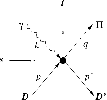
FIG. 1.: Diagram for coherent electromagnetic production of a pseudoscalar particle $\Pi$ on a spin-one particle $D$. The arrows labeled $s$ and $t$ indicate $s$- and $t$-channels.