Off-shell effects on particle production

Abstract

We investigate the observable effects of off-shell propagation of nucleons in heavy-ion collisions at SIS energies. Within a semi-classical BUU transport model we find a strong enhancement of subthreshold particle production when off-shell nucleons are propagated.

During the past 15 years semi-classical transport models have extensively and quite successfully been applied to the description of heavy-ion collisions from SIS to SPS energies (see e.g. Refs. [1, 2]). All these models are based on an on-shell approximation for the nucleons whereas the nucleon resonances are propagated with their spectral functions. However, already at SIS energies the collision rates are so high that this approximation for the nucleons is hard to justify.

While the general formalism to treat also the off-shell transport of particles has been available for quite some while [3, 4, 5] only recently the interest in the in-medium properties of the $\rho$-meson has triggered some new efforts to develop a transport theory that includes dynamical spectral functions (see e.g. [6, 7, 8]). In Ref. [9] we have already presented a model in which the spectral functions of the $\rho$ and $\omega$ mesons are dynamically incorporated and have discussed in detail the transport equation that we solve. It is the purpose of this letter to discuss the effects of collisional broadening also on the spectral functions of the nucleons and thus to treat them on the same footing as the resonances. We also want to report first results on particle production in heavy-ion collisions that were obtained by an inclusion of the nucleonic spectral function.

Since in our method a ’spectral phase space distribution’ plays a central role we specify its precise meaning by starting from the non-relativistic, semi-classical Kadanoff-Baym equation [3]:

$$\left[p_{0}-H_{mf},g^{<}\right]+\left[{\rm Re}g,\Sigma^{<}\right]=-\Sigma^{>}g^{<}+\Sigma^{<}g^{>}\quad,$$ (1)

where the Poisson bracket is given as:

$$\left[X,Y\right]=\frac{\partial X}{\partial x_{\mu}}\frac{\partial Y}{\partial p^{\mu}}-\frac{\partial X}{\partial p_{\mu}}\frac{\partial Y}{\partial x^{\mu}}\quad,$$ (2)

with $x$ and $p$ being the spatial and momentum coordinates. The mean field Hamilton function $H_{mf}$ for the non-relativistic case reads:

$$H_{mf}=\frac{\vec{p}^{2}}{2M_{0}}+{\rm Re}\Sigma\quad,$$ (3)

where $M_{0}$ denotes the mass of the particle and $\Sigma(x,p)$ its retarded self energy that is related to the self energies $\Sigma^{>}$ and $\Sigma^{<}$ which appear in the ’collision term’ on the rhs of Eq. (1) via:

$${\rm Im}\Sigma=\frac{1}{2}(\Sigma^{>}\mp\Sigma^{<})$$ (4)

with the upper sign for bosons and the lower sign for fermions, respectively.

$g^{<}(x,p)$ and $g^{>}(x,p)$ are the Wigner transforms of the real time Greens functions and $g^{<}$ can be interpreted as a generalized phase space density, i.e. the density of particles with 4-momentum $p$ at space time point $x$. The Wigner transform of the retarded Greens function $g(x,p)$ is given by:

$${\rm Im}g=\frac{1}{2}(g^{>}\mp g^{<})\equiv\frac{1}{2}a\quad,$$ (5)

where $a(x,p)$ is the spectral function. $g^{<}$ and $g^{>}$ can be expressed through the spectral function $a$ and a phase space distribution function $f(x,p)$:

$$g^{<} = af$$ (6)

$$g^{>} = a(1\pm f).$$ (7)

For stable particles $f$ reduces to the usual phase space density. From Eq.(1) and the corresponding equation for $g^{>}$ one obtains an algebraic solution for $g$ [3]:

$$g=\frac{1}{p_{0}-\frac{\vec{p}^{2}}{2M_{0}}-\Sigma}.$$ (8)

The spectral function is then given as:

$$a=\frac{\Sigma^{>}\mp\Sigma^{<}}{(p_{0}-\frac{\vec{p}^{2}}{2M_{0}}-{\rm Re}\Sigma)^{2}+\frac{1}{4}(\Sigma^{>}\mp\Sigma^{<})^{2}}.$$ (9)

For a thermally equilibrated system $f$ reduces to the usual Fermi-Dirac or Bose-Einstein distribution function; the non-trivial spectral information is then contained in $a$.

In the following we will neglect the second Poisson bracket of ${\rm Re}g$ and $\Sigma^{<}$ on the lhs of Eq. (1). Its influence on the description of heavy-ion collisions is hard to estimate because a numerical implementation of its effect is not available so far.

Instead of the non-relativistic Hamilton function Eq. (3) we use, in our specific numerical realization [10], the following one:

$$H_{mf}=\sqrt{(\mu+S)^{2}+\vec{p}^{2}}\quad,$$ (10)

where $S(x,p)$ is an effective scalar potential and $\mu$ is a mass parameter that is related to the energy $p_{0}$ via:

$$p_{0}=H_{mf}.$$ (11)

In the following we will express all quantities as function of $\mu$ instead of $p_{0}$. We, therefore, instead of $g^{<}$ use a spectral distribution function $F(\vec{r},t,\vec{p},\mu)$ defined by:

$$Fd\mu\equiv g^{<}\frac{dp_{0}}{2\pi}$$ (12)

and use instead of the spectral function from Eq. (9) the following relativistic one:

$${\cal A}(\vec{r},t,\vec{p},\mu)=\frac{2}{\pi}\frac{\mu^{2}\Gamma_{tot}(\vec{r},t,\vec{p},\mu)}{(\mu^{2}-M_{0}^{2})^{2}+\mu^{2}\Gamma^{2}_{tot}(\vec{r},t,\vec{p},\mu)}\quad,$$ (13)

where the total width in the rest frame of the particle $\Gamma_{tot}$ is given as:

$$\Gamma_{tot}=\frac{p_{0}}{\mu}(\Sigma^{>}\mp\Sigma^{<}).$$ (14)

The transport equation then reads:

$$(\frac{\partial}{\partial t}+\frac{\partial H_{mf}}{\partial\vec{p}}\frac{\partial}{\partial\vec{r}}-\frac{\partial H_{mf}}{\partial\vec{r}}\frac{\partial}{\partial\vec{p}})F=\Sigma^{<}(1\pm f){\cal A}-\Sigma^{>}F.$$ (15)

The collision term is given as:

$$\Sigma^{<}(1\pm f){\cal A}-\Sigma^{>}F=\frac{1}{2E}\int\frac{d^{3}p_{2}d\mu_{2}}{(2\pi)^{3}2E_{2}}\ \frac{d^{3}p_{3}d\mu_{3}}{(2\pi)^{3}2E_{3}}\ \frac{d^{3}p_{4}d\mu_{4}}{(2\pi)^{3}2E_{4}}\ \times$$ (18)

$$\times(2\pi)^{4}\delta^{(4)}(p+p_{2}-p_{3}-p_{4})\left|{\cal M}\right|^{2}\left\{F_{3}F_{4}(1\pm f_{2}){\cal A}_{2}(1\pm f){\cal A}-\right.$$

$$\left.-FF_{2}(1\pm f_{3}){\cal A}_{3}(1\pm f_{4}){\cal A}_{4}\right\}\quad,$$

where $F_{i}\equiv F(\vec{r},t,\vec{p}_{i},\mu_{i})$ and ${\cal A}_{i}$, $f_{i}$ are denoted analogously.

We solve the transport equation (15) by a so-called test particle method, i.e. the distribution function $F$ is discretized in the following way:

$$F(\vec{r},t,\vec{p},\mu)\propto\sum_{i}\delta(\vec{r}-\vec{r}_{i}(t))\delta(\vec{p}-\vec{p}_{i}(t))\delta(\mu-\mu_{i}(t))\quad,$$ (19)

where $\vec{r}_{i}(t)$, $\vec{p}_{i}(t)$, and $\mu_{i}(t)$ denote the spatial coordinate, the momentum and the mass of the test particle $i$, respectively. By inserting this ansatz into the lhs of Eq. (15) one obtains the usual equations of motion for the test particles between collisions:

$$\frac{d\vec{r}_{i}}{dt} = \frac{\partial H_{mf}}{\partial\vec{p}}$$ (20)

$$\frac{d\vec{p}_{i}}{dt} = -\frac{\partial H_{mf}}{\partial\vec{r}}$$ (21)

$$\frac{d\mu_{i}}{dt} = 0.$$ (22)

A formal generalization of the transport equation to a system with different particle species is straightforward. One obtains a transport equation for each particle species that is coupled to all others via the mean field potential and the collision term. In our transport model all baryonic resonances up to about 2 GeV as well as all low lying meson states are explicitly propagated. For a detailed description of the model we refer to Refs. [9, 10]. The actual collision term for the nucleons is thus much more general than the one in Eq. (18) and a numerical solution is only possible by making some approximations that we will describe in the following.

We neglect any medium modifications of total cross sections and decay widths except of Pauli blocking of the outgoing nucleons. The cross sections are calculated as function of the ’free’ invariant energy $\sqrt{s}_{free}$ which is given as:

$$\sqrt{s}_{free}=\sqrt{\mu_{1}^{2}+p_{cm}^{2}}+\sqrt{\mu_{2}^{2}+p_{cm}^{2}}\quad,$$ (23)

where $\mu_{1}$ and $\mu_{2}$ are the masses of the incoming particles and $p_{cm}$ denotes their cms 3-momentum. For invariant energies below $2M_{N}$ we assume the cross section to be constant. We have checked that our results do not change when we use the elastic nucleon-nucleon cross section as function of $\sqrt{s}_{free}-\mu_{1}-\mu_{2}$ instead of as function of $\sqrt{s}_{free}$. The in-medium spectral functions of the produced particles enter only in the determination of the 4-momenta of the outgoing particles. For 2 particles in the final state the masses and the production angle are chosen according to

$$\frac{dn}{d\Omega d\mu_{3}d\mu_{4}}\propto W(\theta)p_{f}{\cal A}_{3}{\cal A}_{4}\quad,$$ (24)

where $W(\theta)$ denotes the respective angular distribution and $p_{f}$ is the cms final state momentum of the outgoing particles with masses $\mu_{3}$ and $\mu_{4}$.

Because in an actual simulation it is practically impossible to obtain statistics for a determination of the collision rate in 8-dimensional phase space we calculate the collision width of the nucleons that enters the spectral functions in Eq. (24) only as function of total momentum in the local rest frame $p_{lrf}$, density $\rho$ and temperature $T$:

$\displaystyle\Gamma_{N}(\vec{r},t,\vec{p},\mu)\to\Gamma_{N}(p_{lrf},\rho(\vec{r}(t)),T(\vec{r}(t))).$The temperature is determined by assuming a Fermi-Dirac distribution from the local $<p^{2}>$ of the test particles. The width is calculated with the nucleon-nucleon cross sections described in Ref. [10] where we take into account Pauli blocking for the elastic part (see e.g. Ref. [9] for details on the calculation of the collisional widths). In Fig. 1 we show the width of the nucleons as function of momentum and temperature at density $2\rho_{0}$. One sees that the width is of the order of 300 MeV for a temperature of 100 MeV and a momentum of 1 GeV and therefore non-negligible. We have checked that the actual collision rates (time integrated and averaged over momentum) in the simulation agree very well with these widths. This holds also for the early, non-equilibrium stages of the collision because the collision rates depend mainly on the density and the momentum. We also find that it is essential to keep the rather strong momentum dependence of the widths, depicted in Fig. 1.

In Ref. [9] we have discussed in detail that the transport equation Eq. (15) does not give the correct asymptotic solutions for particles that are stable in vacuum because a collision broadened particle does not automatically lose its collisional width when being propagated out of the nuclear environment. In Ref. [9] we have introduced a simple scheme to restore the asymptotic width by adding a scalar potential to the equations of motion for the test particles that shifts a particle on its mass shell when it propagates to the vacuum. In order to fulfill energy conservation in case of a system of off-shell nucleons we have to take into account the back coupling of the potential on the other nucleons that create the potential via the density. For a testparticle $i$ this restoring potential is defined as:

$$s_{i}(\vec{x}_{i}(t),t))=(\mu_{i}(t_{cr})-\mu_{vac}-\bar{s}(\vec{x}_{i}(t_{cr}),t_{cr}))\frac{\rho(\vec{x}_{i}(t),t)}{\rho(\vec{x}_{i}(t_{cr}),t_{cr})}\quad,$$ (25)

where $t_{cr}$ denotes the time when the particle is produced; for nucleons we have $\mu_{vac}=M_{N}$. The mass $\mu_{i}$ is then given as:

$$\mu_{i}(t)=\mu_{vac}+s_{i}(\vec{x}_{i}(t),t)+\bar{s}(\vec{x}_{i}(t),t).$$ (26)

In addition to the scheme in Ref. [9] we have included the back coupling potential $\bar{s}$ which is given as:

$$\bar{s}(\vec{r},t)=\frac{1}{2}\frac{\int d^{3}pd\mu(\mu-\mu_{vac})F(\vec{r},t,\vec{p},\mu)}{\int d^{3}pd\mu F(\vec{r},t,\vec{p},\mu)}.$$ (27)

This prescription can be formulated in terms of a modification of the equations of motion for the testparticles:

$$\frac{d\mu_{i}}{dt}=\frac{\mu_{i}-\mu_{vac}-\bar{s}}{\rho}\frac{d\rho}{dt}\approx\frac{\mu_{i}-\mu_{vac}-\bar{s}}{\Gamma_{coll}}\frac{d\Gamma_{coll}}{dt}\quad,$$ (28)

where in the last step we have assumed that the collisional width $\Gamma_{coll}(t)\propto\rho(t)$. Since $s_{i}$ and $\bar{s}$ enter the equations of motion as usual potentials we also get a respective modification of Eq. (21):

$$\frac{d\vec{p}_{i}}{dt}=-\frac{\mu+S}{p_{0}}\left(\frac{\partial S}{\partial\vec{r}}+\frac{\mu-\mu_{vac}-\bar{s}}{\Gamma_{coll}}\frac{\partial\Gamma_{coll}}{\partial\vec{r}}+\frac{\partial\bar{s}}{\partial\vec{r}}\right).$$ (29)

This procedure conserves total energy since $\bar{s}$ is the local average of the $s_{i}$’s. Numerically we obtain energy conservation on a level better than 1% whereas a neglect of the back coupling potential $\bar{s}$ leads to a violation of total energy conservation by about 10%. However, for the calculations of particle yields presented here the inclusion of the restoring potential Eq. (25) is only of minor importance as will be shown below. Because of this it is not essential to what extent our prescription mimicks the effect of the Poisson bracket that we neglected in Eq. (1). We note that the transport equation (1) is based on a first order gradient expansion and therefore does not necessarily need to give the correct asymptotic solutions if the gradients are too large. If the gradients are low enough already the collision term shifts the particles on mass shell as we discussed in Ref. [9].

In the following we exemplarily present results of the present formalism for central Au+Au collisions at 1 AGeV bombarding energy. We have checked that the observed effects are similar for larger impact parameters and smaller systems. The results that we show here were obtained with an EOS that has a compressibility $K$ of 380 MeV. With a softer EOS ($K$=215 MeV) the effects of off-shell nucleons are quantitatively the same. In these calculations we employ a (somewhat arbitrary) lower mass cut-off of 400 MeV to avoid unphysical test particle velocities. The results are stable when this cutoff is varied.

In Fig. 2 we show the mass differential spectrum of the nucleons for different times of the reaction:

$$\frac{dN}{d\mu}(t)=\int\frac{d^{3}p}{(2\pi)^{3}}d^{3}rF(\vec{r},t,\vec{p},\mu)\quad,$$ (30)

where we only count the nucleons that suffered at least from one collision since the others contribute to a $\delta$-function at the pole mass. The upper part of the figure displays the result without the potential Eq. (25). One sees that the nucleon distribution at the end of the collision ($t=40$ fm) is quite strongly peaked around the nucleon pole mass (FWHM$\approx$10 MeV). However, there is still some quite broad tail of low mass nucleons. The inclusion of the potential Eq. (25) ’cures’ this problem (lower part of Fig. 2). One should note here that the spectral distribution in the high density phase of the reaction is hardly affected by the potential. The distribution has a width in the order of 200 MeV which again stresses that an on-shell approximation for the nucleons is hard to justify. It is an essential property of these spectral distributions that they are strongly asymmetric, with an increase towards lower masses. This stems mainly from available phase space which gets larger for smaller masses even without the factor $p_{f}$ in Eq. (24). We stress again that this is a consequence of the collisions and not of the potential (25).

In Fig. 3 (upper part) we show that the off-shell propagation has a quite large influence on the pion spectrum. The number of high energy pions is increased by about a factor 2. There are essentially two reasons for this result. First, in the initial stages of the collision high mass nucleons can be produced which contribute to high energy secondary collisions. This is the effect which has been considered in Ref. [11]. Secondly, outgoing nucleons can have low masses so that effectively the ’temperature’ increases. This allows to produce heavier baryonic resonances in $NN\to NR$ and more energetic pions in $R\to N\pi$. We note that also in the quantummechanical off-shell investigation of Ref. [12] a higher particle yield is obtained when in-medium correlations are taken into account.

In the calculation of these results we have used the free $\Delta$ spectral function; in the population the correct phase space factor has been taken into account. We have ascertained that using the in-medium widths of Ref. [13] in the population of the $\Delta$ made no significant difference.

The lower part of Fig. 3 shows our result for the $K^{+}$-spectrum where we see that the off-shell propagation gives an enhancement by about a factor 2. This enhancement is solely caused by the increase of high energy baryon-baryon and pion-baryon collisions since we do not modify the total production cross sections. This would even lead to a further increase of kaon production because in $BB\to NYK$ a finite width of the outgoing nucleon lowers effectively the production threshold.

The potential Eq. (25) (with $\bar{s}$=0) has only a small effect both on the pion and on the kaon spectrum as can be seen by comparing the dashed and the dotted curves in Fig. 3. This is so because in the high density phase, when the high energy mesons are produced, the collision rates for the nucleons are so large that the nucleons do not travel through a relevant density gradient for which the potential would become important. The potential mainly shifts the low mass tail of nucleons on mass shell during later stages of the collision. For subthreshold particle production the exact mechanism how particles in heavy collision come to their mass shell plays only a minor role. The calculation which includes the backcoupling potential Eq. (27) and thus conserves total energy gives practically the same result (dash-dotted curves in Fig. 3).

We shortly want to mention a few possible improvements for future work. By using vacuum cross sections and vacuum decay widths, as it is always done in transport calculations, detailed balance is violated when off-shell nucleons are propagated. This could only be cured by working with amplitudes instead of parameterizations of cross sections and decay widths which would enhance the numerical effort dramatically. However, we do not expect the violation of detailed balance to be significant for our present results because the harder particles for which the increase due to off-shell effects is most pronounced (Fig. 3) are produced in the first hard collisions. Furthermore, in all transport calculations the analyticity of the self energy $\Sigma$ is neglected and the mean field potential that enters into the drift term is determined independently of the self energies $\Sigma^{<}$ and $\Sigma^{>}$ in the collision term. For off-shell transport this analyticity might be important for the mechanism how the particles come to their mass shell when they travel to the vacuum. In principle, we should also take into account a dynamical spectral function for the pion since its collision rates are even larger than the ones of the nucleons.

In summary, we have presented a first calculation of nucleonic spectral functions in a transport theoretical framework and have exploited their effects on particle production in heavy-ion collisions at SIS energies. We have found large effects compared to a calculation with an on-shell approximation for the nucleons. We thus hope that this work will stimulate future, more refined work on the influence of off-shell properties on particle production yields in heavy-ion collisions.

The authors would like to thank C. Greiner, J. Knoll, V. Koch, A. Larionov, and S. Leupold for discussions and helpful comments on the manuscript. They also acknowledge a critical reading of the manuscript and lively arguments with W. Cassing.

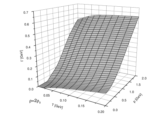
FIG. 1.: The nucleon width as function of momentum $p$ and temperature $T$ at density $\rho=2\rho_{0}$.

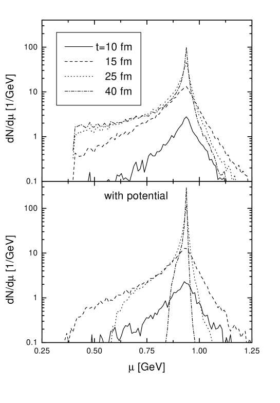
FIG. 2.: Spectral distribution of nucleons for Au+Au at 1 AGeV. In the lower part the restoring potential from Eq. (25) was included (without the backcoupling potential $\bar{s}$).

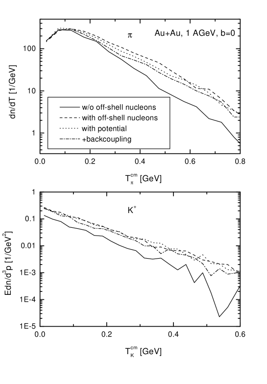
FIG. 3.: Effect of off-shell propagation of nucleons on pion (upper part) and kaon (lower part) spectra. For the dotted lines the restoring potential from Eq. (25) was included. For the dash-dotted lines the energy-conserving backcoupling potential Eq. (27) was additionally taken into account.

REFERENCES

- [1] W. Cassing and E.L. Bratkovskaya, Phys. Rep. 308, 65 (1999).
- [2] S.A. Bass et al., Prog. Part. Nucl. Phys. 41, 225 (1998).
- [3] L.P. Kadanoff and G. Baym, Quantum statistical mechanics, Benjamin, New York, 1962.
- [4] P. Danielewicz, Ann. Phys. (N.Y.) 152, 239 (1984).
- [5] W. Botermans and R. Malfliet, Phys. Rep. 198, 115 (1990).
- [6] J. Knoll, Prog. Part. Nucl. Phys. 42, 177 (1999).
- [7] W. Cassing and S. Juchem, nucl-th/9903070.
- [8] Yu.B. Ivanov, J. Knoll, and D.N. Voskresensky, nucl-th/9905028.
- [9] M. Effenberger, E.L. Bratkovskaya, and U. Mosel, nucl-th/9903026.
- [10] S. Teis, W. Cassing, M. Effenberger, A. Hombach, U. Mosel, and Gy. Wolf, Z. Phys. A 356, 421 (1997).
- [11] G.F. Bertsch and P. Danielewicz, Phys. Lett. B 367, 55 (1996).
- [12] P. Bozek, Phys. Rev. C 56, 1452 (1997).
- [13] M. Effenberger, A. Hombach, S. Teis, and U. Mosel, Nucl. Phys. A613, 353 (1997).