Covariance of Antiproton Yield and Source Size in Nuclear Collisions

Abstract

We confront for the first time the widely-held belief that combined event-by-event information from quark gluon plasma signals can reduce the ambiguity of the individual signals. We illustrate specifically how the measured antiproton yield combined with the information from pion-pion HBT correlations can be used to identify novel event classes.

]

I introduction

Signals of novel phenomena from hadron production in relativistic heavy ion experiments have proven ambiguous at the Brookhaven AGS and the CERN SPS, primarily because descriptions of the ‘ordinary’ hadron production mechanisms are under-constrained. It has long been conjectured – but not yet demonstrated – that the added information from the correlation of distinct signals can reduce the ambiguity of the individual signals. In particular, the measurement of such correlations is one of the driving principles behind the PHENIX and STAR experiments at RHIC [1]. However, to describe the correlated information that these experiments yield, phenomenologists must introduce new unconstrained parameters.

We propose that added information can in fact be gained by studying antiproton production in conjunction with pion interferometry, HBT, on an event-by-event basis. Various authors have suggested that both antiproton production [2] and HBT radius parameters [3] can change abruptly and dramatically if quark gluon plasma forms in a heavy ion collision. However, theoretical uncertainties [4, 5, 6] and experimental difficulties [7] have made results difficult to interpret in that context. In this paper, we demonstrate the utility of covariance measurements by constructing a plausible scenario in which a measurement of the covariance of these observables can resolve ambiguity in individual HBT and antiproton measurements. After explaining the basic scenario, we discuss how antiproton production and HBT radii become correlated in the framework of a thermal model of hadron production. We then develop a Monte Carlo code to provide a realistic simulation of our scenario in the context of STAR.

Measurements of the covariance of distinct signals are useful when event averaging hides otherwise-strong signatures of a new event class. Suppose that there are two event classes – “plasma” and “hadronic.” Further assume that the mean antiproton rapidity density $\overline{N}\equiv d{\overline{n}}/dy$ is different in each class, so that the signal is truly strong. Averaging over events yields

$$\langle\overline{N}\rangle\equiv\sum_{i}\overline{N}_{i}=f\overline{N}(q)+(1-f)\overline{N}(h),$$ (1)

where the $f$ is the probability that the $i^{\rm th}$ collision forms a plasma and ${\overline{N}}(q,h)$ are the average values for the plasma and hadronic classes respectively. The event-averaged $\langle\overline{N}\rangle$ is a smooth function of centrality and beam energy, because $f$ is a continuous function of the collision geometry and energy deposition. Smooth data sets, such as those in figs. 1a and 1b, are subject to broad interpretation.

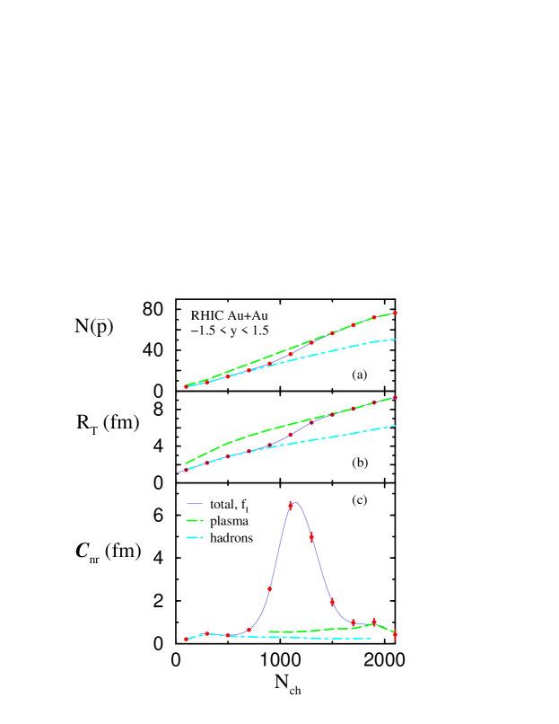
FIG. 1.: Antiproton multiplicity (a), pion HBT transverse radius (b) and their covariance (c) as functions of the charged particle multiplicity. Results are obtained from simulations below for the scenario I, cf. eq. (28). Multiplicities are computed for the STAR acceptance.

The correlation of ${\overline{N}}$ with the HBT transverse radius $R_{T}$ can betray the existence of the new event class. This correlation is characterized by the covariance:

$${\cal C}_{nr}\equiv\sum_{i}(\overline{N}_{i}-\langle\overline{N}\rangle)(R_{Ti}-\langle R_{T}\rangle),$$ (2)

where $R_{T}$ is the transverse radius measured in event-by-event pion interferometry. We find

$$\Delta{\cal C}_{nr}=f(1-f)\{\overline{N}(q)-\overline{N}(h)\}\{R_{T}(q)-R_{T}(h)\},$$ (3)

where ${\cal C}\equiv f{\cal C}(q)+(1-f){\cal C}(h)+\Delta{\cal C}$ and the covariance for each class is ${\cal C}({q,h})$. The term $\Delta{\cal C}$ depends on the hidden shift in $\overline{N}$ and $R_{T}$. In the best of all possible worlds, $f$ will change from zero to unity for a single target-projectile combination as the impact parameter $b$ is varied. This variation can introduce a peak as shown in fig. 1c, provided that both class-averages $R_{T}(q)$ and $\overline{N}(q)$ truly exceed the hadronic values, as predicted. More likely, one may come upon a low impact-parameter region where $f$ begins to rise, or a peripheral region where $f$ begins to fall.

We point out that the variances $\sigma_{\overline{N}}^{2}$ and $\sigma_{R_{T}}^{2}$ can exhibit similar behavior in the presence of two event classes. For antibaryons, we find $\langle\Delta\overline{N}^{2}\rangle=f\sigma_{\overline{N}}^{2}(q)+(1-f)\sigma_{\overline{N}}^{2}(h)+\Delta\sigma_{\overline{N}}^{2}$, where

$$\Delta{\sigma_{\overline{N}}}^{2}=f(1-f)\{\overline{N}(q)-\overline{N}(h)\}^{2},$$ (4)

and $\sigma_{\overline{N}}^{q,h}$ are the standard deviations for each class; the result for $R_{T}$ is similar. The variance $\sigma_{\overline{N}}^{2}$ can be particularly interesting in the context of recent work by Stephanov, Rajagopal and Shuryak [8]; we address that point elsewhere [9, 10].

A measurement of (2) is built upon an event-by-event analysis on which we now comment. We expect anywhere from 50 to 100 antiprotons per event in the STAR acceptance, and possibly more [11]. Such a number is perfectly adequate for event-by-event analysis. Since our intent is to use the antiproton yield as a proxy for an antibaryon measurement, we are not concerned if the measurements contain a contribution from antilambdas, as found at the AGS [7]. On the other hand, the HBT part of the measurement is challenging because it involves an event-by-event two-pion correlation analysis. In an HBT analysis, one compares the measured identical-pion correlation function $C_{\pi\pi}$ to a Gaussian parameterization. Radius parameters are typically obtained by a three dimensional fit to high-statistics data (see [4] for details). The hadronization of the plasma affects these spacetime-dependent variables directly by delaying the freezeout of the system [3]. While such a three-dimensional analysis may not be practical for single RHIC events, the feasibility of one dimensional analyses has been studied by the STAR experiment [12]. One can extract the transverse radius by comparing

$$C_{\pi\pi}(q_{T})=1+{\rm e}^{-q_{T}^{2}R_{T}^{2}}$$ (5)

to data, where $q_{T}$ is the difference in the pions’ transverse momenta. Alternatively, Heinz and Wiedemann suggest that it may be easier to extract event-by-event parameters using $R_{T}^{-2}\propto\int d^{2}q_{T}q_{T}^{2}(C(q_{T})-1)$ [13]. The difference between these definitions is immaterial to our discussion. However, we point out that $R_{T}$, which essentially measures the transverse system size, is not an ideal plasma probe. Nevertheless, we find a strong change in ${\cal C}_{nr}$ for a $50\%$ increase in $R_{T}(q)$ due to the transverse growth of the longer-lived plasma system.

II Fluctuations near equilibrium

To establish the mechanisms that drive the correlations and fluctuations in antibaryon production and pion HBT, we employ the idealized but standard Bjorken hydrodynamic framework that describes particle production near rapidity $y=0$. We assume that matter in this region is in local thermal equilibrium, with an average local temperature $T$, entropy density $s$ and net baryon density $\rho_{B}$ that vary only with proper time $\tau$. The transverse area $\cal A$ is initially determined by the overlap of the colliding nuclei. One can define a comoving volume for matter in the central region, $V\equiv S/s={\cal A}\tau$. This volume grows from a formation time $\tau_{0}$ to freezeout at $\tau_{F}$, so that the entropy per unit rapidity for all hadrons $S$ is $\tau$ independent. The total rapidity density of hadrons $N_{\rm tot}$ is nearly constant, because $N_{\rm tot}\propto S$ for a system dominated by light hadron species with masses $\ll T$. Baryon current conservation implies that the net baryon rapidity density $N_{B}\equiv dn_{B}/dy={\cal A}\rho_{B}(\tau)\tau$ is independent of proper time. Mean rapidity densities of individual species, such as antibaryons $\overline{N}$ and baryons $N$, vary with $\tau$. Observe that this model is distinct from global equilibrium models used by many groups. The key distinction is that here, we focus on thermodynamic quantities local to the central region.

In local equilibrium, the number of antibaryons at midrapidity and the source size fluctuate depending on the fluctuation of the state variables in this region. We consider an ensemble of collisions at fixed impact parameter in which $V$, $T$ and $N_{B}$ fluctuate [14]. We assume that these variables are independently established near $y=0$ in the preequilibrium evolution, so that they are statistically independent. The comoving volume and temperature fluctuate because the initial number of mesons and the initial energy per meson vary from event to event. The net baryon number fluctuates because the central region can exchange baryon current with the rest of the collision volume for fixed $V$ and $T$, i.e. the central region is held at constant baryon chemical potential. We remark that this ensemble differs marginally from the familiar Grand Canonical ensemble, in which the total hadron energy fluctuates and $T$ is held fixed. The differences are negligible in the regime $N_{B}\ll N_{\rm tot}$ that we consider.

The fluctuations of a quantity $X$ are characterized by the variance $\sigma_{X}^{2}=\langle\Delta X^{2}\rangle$ for $\Delta X\equiv X-\langle X\rangle$. The fluctuations of $V$ satisfy

$${{\sigma_{V}^{2}}\over{V^{2}}}={{\sigma_{\rm tot}^{2}}\over{N_{\rm tot}}}\sim N_{\rm tot}^{-1},$$ (6)

where $N_{\rm tot}$ is the total number of hadrons. Thermal fluctuations satisfy [14]:

$$\sigma_{T}^{2}\approx T^{2}C_{v}^{-1}\approx{T^{2}\over{12}}~{}{{\sigma_{V}^{2}}\over{V^{2}}}$$ (7)

for a system of a heat capacity $C_{v}$, where the second equality follows for an ideal gas of (mostly) massless hadrons in which $N_{B}\ll N_{\rm tot}$ and Fermi and Bose statistics can be neglected. The variance of the net baryon number at constant temperature and volume is

$$\sigma_{B}^{2}\equiv\langle\Delta N_{B}^{2}\rangle_{{}_{TV}}=T\partial N_{B}/\partial\mu_{B}$$ (8)

by straightforward extension of ref. [14]. For an ideal gas, ${\overline{N}}=Vf(T)\exp(-\mu_{B}/T)$ and $N_{B}=2Vf(T)\;{\rm sinh}(\mu_{B}/T)$ (we need not specify $f$), implying that

$$\sigma_{B}^{2}=N+\overline{N},$$ (9)

neglecting small corrections from Fermi statistics.

We comment that Stephanov, Rajagopal and Shuryak [8] have discussed thermal fluctuations of observables at a critical end point, focusing on the effect of the divergence of $C_{V}$ on (7). We point out that critical fluctuations also affect (8), because $\partial N_{B}/\partial\mu_{B}=-\partial^{2}\Omega/\partial\mu^{2}$ diverges at that point, where $\Omega$ is the free energy. The antibaryon fluctuations that we discuss shortly would reflect this critical behavior, c.f. (12) below. Here, we assume that $T$ and $\mu_{B}$ are sufficiently far from that point that these effects are negligible.

The extent to which the number of antibaryons fluctuates depends on whether or not chemical equilibrium holds with respect to the reactions that change the number of baryon-antibaryon pairs, e.g. $N{\overline{N}}\rightleftharpoons$ mesons. We do not expect chemical equilibrium for these processes unless a plasma is formed [15]. Suppose then that the numbers of baryons and antibaryons are individually conserved. For constant $T$ and $V$, ref. [14] implies that the antibaryons essentially follow Poisson statistics,

$$\langle\Delta\overline{N}^{2}\rangle_{{}_{TV}}=\overline{N},\,\,\,\,\,\,\,\,\,\,\,\,\,\,\,\,\,\,\,\,{\rm no~{}chemical~{}equilibrium}$$ (10)

with a similar expression for protons. Observe that HIJING and similar event generators exhibit exactly the same Poisson-like behavior (such behavior is built in to these models).

Chemical equilibrium couples fluctuations of the baryons to those of the antibaryons, reducing the relative variance compared to (10). In this case, a small change in the number of antibaryons requires the net baryon number change:

$$\Delta\overline{N}=\left({{\partial{\overline{N}}/\partial\mu_{B}}\over{\partial N_{B}/\partial\mu_{B}}}\right)\Delta N_{B}.$$ (11)

The variance in antibaryons is then

$$\langle\Delta\overline{N}^{2}\rangle_{{}_{TV}}=T{{(\partial{\overline{N}}/\partial\mu_{B})^{2}}\over{\partial N_{B}/\partial\mu_{B}}}=\overline{N}^{2}(N+\overline{N})^{-1},$$ (12)

where we have used (9). Note that we recover (10) in the limit $N\ll\overline{N}$, since baryon conservation keeps $\overline{N}$ constant.

Volume and thermal fluctuations can also cause the number of antibaryons to fluctuate. We write:

$$\Delta\overline{N}={{{\overline{N}}\Delta V}\over{V}}+\left({{\partial{\overline{N}}}\over{\partial T}}\right)_{{}_{N_{B}}}\!\!\!\!\Delta T+\left({{\partial{\overline{N}}}\over{\partial N_{B}}}\right)_{{}_{T}}\Delta N_{B}.$$ (13)

The third contribution represents the constant T and V results discussed earlier. The second term,

$$\left({{\partial{\overline{N}}}\over{\partial T}}\right)_{{}_{N_{B}}}={{\partial{\overline{N}}}\over{\partial T}}-\left({{\partial{\overline{N}}}\over{\partial\mu_{B}}}\right){{\partial N_{B}/\partial T}\over{\partial N_{B}/\mu_{B}}},$$ (14)

allows thermal fluctuations to change the antibaryon population by making pairs in chemical equilibrium; it strictly vanishes otherwise. We will see that the covariance (2) arises from the first term.

For an ideal gas in chemical equilibrium,

$${{\Delta\overline{N}}\over{\overline{N}}}={{\Delta V}\over{V}}+{{2\epsilon N}\over{N+\overline{N}}}{{\Delta T}\over T}-{{\Delta N_{B}}\over{N+\overline{N}}}.$$ (15)

where $\epsilon=E_{\overline{N}}/\overline{N}T\approx m/T+3/2$ is the energy per antibaryon per unit temperature. We then obtain:

$${{\sigma_{\overline{N}}^{2}}\over{\overline{N}^{2}}}={{\sigma_{V}^{2}}\over{V^{2}}}+\epsilon^{2}\left({{2\overline{N}}\over{N+\overline{N}}}\right)^{2}{{\sigma_{T}^{2}}\over{T^{2}}}+{{\sigma_{B}^{2}}\over{(N+\overline{N})^{2}}}.$$ (16)

The third term, i.e. (12), dominates the antibaryon fluctuations when $N_{\rm tot}\gg N+\overline{N}$, as eqs. (6,7) suggest. For $\overline{N}\gg N$ we obtain the generalization of (10),

$${{\sigma_{\overline{N}}^{2}}\over{\overline{N}^{2}}}={{\sigma_{V}^{2}}\over{V^{2}}}+{1\over{\overline{N}}}.\,\,\,\,\,\,\,\,\,\,{\rm no~{}chemical~{}equilibrium}$$ (17)

The underlying volume fluctuations follow (6) provided that thermal equilibrium holds.

We expect volume, thermal and baryon-number contributions to be generally comparable at RHIC in thermal equilibrium. The sum of the volume and thermal terms is roughly $1+\epsilon^{2}/12\approx 7$ for $T=140$ MeV and $m=938$ MeV, implying a contribution to $(\sigma_{\overline{N}}/\overline{N})^{2}$ of $\sim 0.7\%$ for $N_{\rm tot}\sim 10^{3}$ as expected in Au+Au collisions. Baryon density fluctuations contribute $\sim 1.3\%$ to the variance for $\overline{N}\approx N\approx 40$, yielding a total $(\sigma_{\overline{N}}/\overline{N})^{2}\sim 2\%$. Observe that either the chemical nonequilibrium result (10) or HIJING would give a similar value $\sim 2.5\%$.

We expect the covariance (2) to be determined primarily by volume fluctuations, as we see by computing the related covariance of $\overline{N}$ and $V$,

$${\cal C}_{nv}\equiv\langle\Delta\overline{N}\Delta V\rangle=\overline{N}\sigma_{V}^{2}/V.$$ (18)

The large contributions to the antibaryon variance (16) from net baryon number and temperature fluctuations are absent in (18). A very important consequence of this result is that this expression is valid whether or not chemical equilibrium holds.

To relate the volume fluctuations to fluctuations in the HBT radius, we observe that variations in HBT transverse radius are driven primarily by the geometrical effective radius $\sim{\cal A}^{1/2}$ and, secondarily, by flow [5]. By analogy with (13), we make the phenomenological ansatz:

$$\Delta R_{T}/R_{T}=\kappa\Delta V/2V+\lambda\Delta T/T,$$ (19)

where the parameters $\kappa=2\partial\log R_{T}/\partial\log V$ and $\lambda=\partial\log R_{T}/\partial\log T$ generally must be determined by hydrodynamic calculations. We take the relative concentrations $N/N_{\rm tot}$ and $\overline{N}/N_{\rm tot}$ to be small enough that the baryons have a negligible effect on the flow at RHIC. The covariance of $R_{T}$ and $\overline{N}$ is then

$${\cal C}_{nr}\equiv\langle\Delta{\overline{N}}\Delta R_{T}\rangle=\overline{N}R_{T}\left(\kappa{{\sigma_{V}^{2}}\over{2V^{2}}}+\epsilon\lambda{{\sigma_{T}^{2}}\over{T^{2}}}\right),$$ (20)

while the fluctuations in $R_{T}$ itself satisfy

$$\sigma_{R_{T}}^{2}/R_{T}^{2}\equiv\kappa^{2}\sigma_{V}^{2}/4V^{2}+\lambda^{2}\sigma_{T}^{2}/T^{2}.$$ (21)

In contrast to (18), there is no first-principles justification for (20, 21) – flow effects are outside the reach of our thermodynamic approach.

In the absence of transverse flow, $R_{T}$ is essentially the geometric transverse radius [5], so that flow contributions to (20) and (21) must vanish. In keeping with our Bjorken-like scenario, we therefore take

$$\kappa=1\,\,\,\,\,{\rm and}\,\,\,\,\,\lambda=0.$$ (22)

To see that this approximation is reasonable, we use a parameterization of the Yano-Koonin-Podgoretskii radius $R_{T}(M_{T})$, eq. (47) of ref. [5], which is closely related to our $R_{T}$. For that parameterization, $\kappa$ is strictly unity. We estimate $\lambda\sim 0.3$ for a plausible mean transverse fluid rapidity of $\eta_{f}=0.6$. This result is in keeping with findings at SPS energy, where NA49 finds that $R_{T}(M_{T})$ decreases by $\sim 20\%$ as $m_{T}$ is varied from zero to $\approx 0.45$ MeV, corresponding to $\lambda\sim 0.2$. One can improve our estimate by introducing stochastic noise and dissipation into a hydrodynamic model and studying the consequent fluctuation of $R_{T}$.

We comment that by using the comoving volume $V$ for the Bjorken scaling expansion, we can describe the local equilibrium fluctuations in our evolving system as if the system were stationary. However, for more general local equilibrium systems flowing in three dimensions, i.e., real heavy ion systems, we must obtain the variance and covariance from the local hydrodynamic fluctuations [16]. To see how inhomogeneity can affect our estimates, consider temperature fluctuations that locally satisfy $\langle\Delta T({\vec{x}})\Delta T({\vec{x}}^{\prime})\rangle=[T(\vec{x})^{2}/n(\vec{x})c_{v}(\vec{x})]\delta(\vec{x}-\vec{x}^{\prime})$, where $n$ is the total hadron density and $c_{v}$ the specific heat. Let us assume that longitudinal Bjorken scaling holds but that the system is inhomogeneous in the transverse direction $\vec{r}$ – the simplest possible extension of our idealized model. Experimental measurements of the average transverse momentum roughly yield the volume average $T\propto\int d^{2}rn(\vec{r})T(\vec{r})$ in each event [8]. We can then use this volume average to construct the event average $\langle\Delta T^{2}\rangle$. Using the above correlation function, we see that this average satisfies (7), since local equilibrium implies that $T(r)^{2}/c_{v}(r)$ scales as $n^{-1}$, neglecting corrections from Bose and Fermi statistics. In this case and in the case of rapidity densities, we do not expect transverse inhomogeneity to introduce large corrections. However, experiments do not strictly yield the volume average of $T$ but, rather, momentum distributions from which we extract an average $p_{T}$ slopes. To treat fluctuations of $p_{T}$ slopes, $R_{T}$ and other such quantities with precision, we must use hydrodynamic or transport models that include noise and dissipation that respect the fluctuation-dissipation theorem [16]. No such models exist.

III fluctuations in ion collisions

To describe the two-event-class scenario outlined in the introduction, we now apply these general results to develop a Monte Carlo event generator for correlated signals in RHIC collisions. With this generator we can account for additional sources of fluctuations in heavy ion collisions as described below. Schematically, we generate events as follows. For each event class, the average $\overline{N}$, $R_{T}$ and total rapidity density $N_{\rm tot}$ are determined at each impact parameter by the collision geometry using the prescription that we describe shortly. We then generate values of $\overline{N}_{i}$,$R_{Ti}$ and the charged-particle multiplicity for each event in accord with the variances and covariance calculated earlier. As possible in the STAR experiment, we use the charged particle multiplicity to determine the centrality of each event. We then compute the covariance as a function of multiplicity for two illustrative two-class scenarios. In addition, we present the distribution of simulated events to eliminate some of the abstraction that often obfuscates statistical analyses.

In discussing thermodynamic fluctuations, we have so far assumed that collisions occur at a fixed impact parameter $b$, with fluctuations occurring about well defined mean values fixed by $V$, $T$ and $N_{B}$. Additional fluctuations arise in heavy ion experiments, e.g., from the imperfect experimental knowledge of the impact parameter. In this work, we incorporate such fluctuations into our description using a Monte Carlo framework. However, one can understand how these fluctuations come about as follows. Events with impact parameters in the range from $b-\Delta b/2$ to $b+\Delta b/2$ yield average numbers of antibaryons that differ by $\approx(\partial{\overline{N}}/\partial b)\Delta b$. An experiment that does not resolve these impact parameters will measure a covariance:

$${\cal C}_{nr}-{\cal C}_{nr}^{\rm eq}\approx\left({{\partial{\overline{N}}}\over{\partial b}}\right)\left({{\partial R_{T}}\over{\partial b}}\right)\sigma_{b}^{2},$$ (23)

where $\sigma_{b}$ is the standard deviation for events in the unresolved range and ${\cal C}_{nr}^{\rm eq}$ is the average equilibrium contribution for collisions at $b$. This centrality contribution must vanish for central collisions by symmetry. More generally, its magnitude depends on how the mean values $\overline{N}$ and $R_{T}$ vary with collision geometry and, additionally, how centrality is measured. For Au+Au collisions in STAR, we find that impact parameter fluctuations are typically more important than volume fluctuations, but less important than the thermal and baryon-number contributions. [At an impact parameter $b=6$ fm, we use eqs. (24, 26) to estimate the centrality contribution to the relative covariance ${\cal C}_{nr}/{\overline{N}}R_{T}$, to be $\sim 0.3\%$ compared a thermal contribution of $\sim 0.05\%$.]

To estimate antibaryon production for the purely hadronic event class, we observe that kinetic theory estimates suggest that it is unlikely that baryons will reach chemical equilibrium [15, 10]. At RHIC, events too peripheral to produce a plasma will yield fewer antibaryons than required by detailed balance for the reactions $N\overline{N}\rightleftharpoons$ mesons. Chemical equilibration then requires that meson collisions increase the antibaryon population, but time scales for those processes greatly exceed the relevant dynamic time scales. We can therefore expect the hadron fluid to be far from chemical equilibrium, although thermal equilibrium may hold. In this case, the mean rapidity density of antibaryons is essentially the same as its initial value, since antibaryon number is now effectively conserved. Moreover, we use (17) and (18) to compute the standard deviation $\sigma_{\overline{N}}(h)$ and covariance $C_{nr}(h)$. Observe that the final state is practically indistinguishable from the entirely-nonequilibrium initial state. For Au+Au at RHIC we take:

$$\overline{N}(h)\equiv\overline{n}_{h}{\cal N}(b)/{\cal N}(0);$$ (24)

where $\overline{n}_{h}=40$, a value consistent with the range of event generator predictions: HIJING, HIJING/$B{\overline{B}}$ (its successor) and RQMD report rapidity densities of 60, 20 and 20 respectively. We assume the rapidity density varies with impact parameter in proportion to the number of participants, ${\cal N}(b)$, in agreement with HIJING calculations at the 1-2 percent level.

Antiproton production can be very different in a plasma. A variety of mechanisms from chiral restoration to disoriented chiral condensate formation [2] can enhance production of baryon-antibaryon pairs and facilitate equilibration. Model calculations typically yield values of the antiproton rapidity densities well in excess of event generator estimates. For example, ref. [11] predicts values of $\overline{N}$ of about 86, almost three times the HIJING level. For an enhancement at that level to be hidden in the mean value (1), $f$ would have to be very small. We assume a more conservative 30% enhancement over the hadron gas value in a central collision,

$$\overline{n}_{q}\approx 26,$$ (25)

and take the same centrality dependence. Importantly, since chemical equilibration is likely in a plasma, we now use (16) to calculate $\sigma_{\overline{N}}(q)$. On the other hand the covariance for chemical equilibrium is still given by (18), so that $C_{nr}(q)\approx C_{nr}(h)$.

For our HBT estimate, we take a mean transverse radius in the hadronic event to be roughly the geometric radius

$$R_{T}(h)=r_{h}[{\cal A}(b)/{\cal A}(0)]^{1/2},$$ (26)

where $r_{h}=6$ fm and ${\cal A}(b)$ is the geometrical overlap area of the colliding nuclei. For comparison, Hardtke and Voloshin [20] has used RQMD to find a side radius $R_{s}\approx 5$ fm in Au+Au at RHIC and we expect $R_{T}\sim R_{s}$. We then use (20) and (22) to estimate the fluctuations.

Pratt and Bertsch [3] have argued that plasma formation can increase the pion HBT radius parameters, e.g., if a nearly-first-order phase transformation leads to the dramatic increase of the collision-system lifetime and size. However, as noted earlier, this effect is only dimly reflected in $R_{T}$. We assume a $50\%$ increase over the hadronic value,

$$r_{q}\approx 9~{}{\rm fm}.$$ (27)

We expect the intrinsic uncertainty from (21) to be much smaller than the experimental uncertainty.

We assume that STAR will measure the multiplicity of charged pions to select the centrality of each event. We compute the multiplicity for each event assuming a Gaussian distribution with an average value $N_{\rm tot}(b)=N_{\rm tot}(0){\cal N}(b)/{\cal N}(0)$ and a standard deviation $\sigma_{\rm tot}=\sqrt{N_{\rm tot}}$ consistent with thermal equilibrium. The scale $N_{\rm tot}(0)=2100$ is determined by the initial production regardless of event class, in accord with entropy and energy conservation; the particular value is taken from a HIJING simulation in the STAR acceptance. We then generate the antiproton yield and $R_{T}$ using (6), (7), (12) and (18). To each $N_{\overline{p}}\approx\overline{N}/2$ and $R_{T}$ value we add a simulated “experimental” fluctuation. The experimental fluctuation in $R_{T}$ is distributed with $\Delta R/R\sim 10\%$, in accord with [12], while that of $N_{\overline{p}}$ assumes an ad hoc 95% detection efficiency.

Importantly, these experimental fluctuations do not affect the covariance, although they do affect the scatter of events. Only correlated uncertainties in the $\overline{N}$ and $R_{T}$ measurements can alter the covariance. Since these two measurements are very different, we do not anticipate any correlated uncertainty (although real experiments are very complicated!), as long as the measured $\overline{N}$ and $R_{T}$ truly come from the same event.

To illustrate the effect of two event classes, we present two ad hoc scenarios for the onset of plasma events in RHIC Au+Au collisions. We start with a Pangloss scenario in which plasma forms with certainty in all but the most peripheral collisions. The large fluctuations in stopping and energy deposition inherent in peripheral collisions might plausibly result in an event class in which plasma does not form. We take the probability $f(b)$ for plasma events to be

$$f_{\rm I}(b)=\{1+\exp[(b-b_{0})/\Delta b]\}^{-1},$$ (28)

a form that would apply in the best of all possible worlds. The plasma fraction increases from zero to one within a range $\sim 2\Delta b\sim 1$ fm of $b_{0}=6$ fm. In figs. 1a and 1b we show the average $\overline{N}$ and $R_{T}$ derived from 10,000 simulated events. We see that the average values vary smoothly between hadronic and plasma model expectations. In fig. 1c we present the covariance of $R_{T}$ from $10^{6}$ events (STAR will obtain that many events in twelve days). Our simulations clearly establish the behavior of (3) within the statistical uncertainties. Observe that the tails of the distribution are described mainly by (23), with volume fluctuations contributing only at the 10-30% level. Further note that in the limit as $\Delta b\rightarrow 0$, the width of the bump in fig. 1c tends to the value $\sigma_{\rm tot}(b_{0})$ set by the multiplicity distribution.

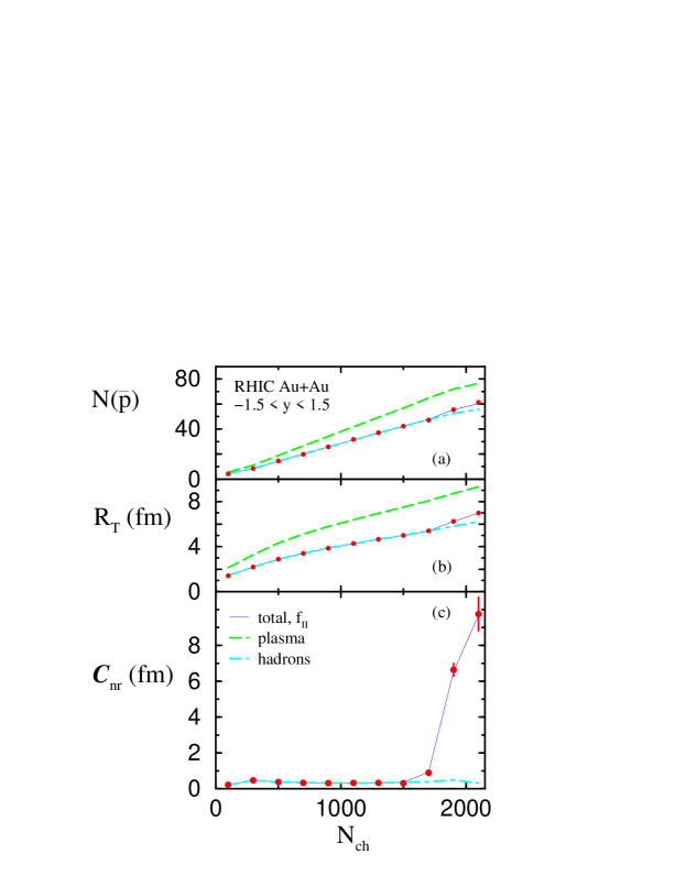
FIG. 2.: Antiproton multiplicity (a), pion HBT transverse radius (b) and their covariance (c) for scenario II, cf. eq.(29).

We now consider a more conservative – but no less ad hoc – scenario in which plasma events appear in only a fraction of the most central collisions. We take:

$$f_{II}(b)=0.25~{}[1-(b/b_{0})^{2}]$$ (29)

for $b<b_{0}=3$ fm, with $f=0$ otherwise. We imagine that a region of $T>T_{C}$ forms in central collisions, and that this region grows in size as collisions become more central. The event-averaged Monte Carlo results in fig. 2a and 2b show no appreciable difference from hadronic expectations, while the covariance in fig. 2c shows a striking enhancement.

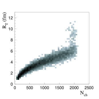
FIG. 3.: Distribution of events: transverse radius vs. charged particle multiplicity for 10,000 simulated events for scenario II.

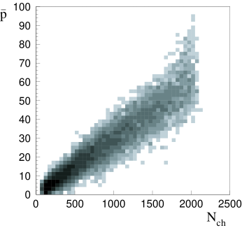
FIG. 4.: Distribution of events: antiproton multiplicity vs. charged particle multiplicity for 10,000 simulated events for scenario II.

To appreciate how the event distribution gives rise to this behavior, we show the distribution of events in scatter plots in figs. 3, 4 and 5. While the antiproton results in fig. 4 are unconvincing, the HBT events in fig. 3 show a hint of a new population in central collisions. The correlated signal from 10,000 events is shown in fig. 5. Here, two event classes are clearly distinguishable. The scatter plot indicates that we can identify the events with the largest antiproton yield as anomalous. Armed with such information, experimenters can then search for an optimal beam energy and target-projectile combination to sweep out the coexistence region as in fig. 1. Moreover, one can introduce an antiproton trigger to other experiments to gather a statistically significant sample of plasma events, e.g., to study hard probes or three dimensional HBT. We point out that the covariance can be measured to arbitrary precision by collecting events and, consequently, is more sensitive to the appearance of a new event class than is the qualitative scatter plot. The result in fig. 2c is computed from $10^{6}$ events.

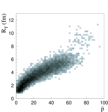
FIG. 5.: Distribution of events: antiproton multiplicity vs. transverse radius for 10,000 simulated events for the scenario II.

In this work, we have assumed that local equilibrium holds, so that all variances and covariances are determined by the equation of state and the conservation laws. When equilibrium is not in force, there are very few constraints on correlations. We study the effect of incomplete chemical equilibrium on the variances and covariances in [10]. While such results can be more realistic, they are also more model dependent. It will eventually be necessary to use models like RQMD, UrQMD, and VNI to study correlated observables. Such models perhaps offer the most realistic description of single particle observables, but may require modification to address event-by-event correlations. For example, it has not been demonstrated that fluctuations in these models respect the fluctuation-dissipation theorem when one imposes the appropriate boundary conditions and approximate local equilbrium [14]. Consequently, it is not clear that the dynamical correlations these models produce are realistic.

On the experimental side, it is not clear how to extract event-by-event HBT radii in practice [12]. If experimental fluctuations in HBT radii are too large, it will be necessary to develop a super-event analysis scheme [21].

We have shown that under the right circumstances a correlated analysis of observables such as antiproton yield and the pion $R_{T}$ will augment the discovery potential for novel event classes. In particular, we stress the importance of looking for systematic changes in correlations as functions of the centrality. A first study of fluctuations of the pion transverse momentum and the $K/\pi$ ratio by the NA49 experiment at the SPS focused on central collisions [17]. Their study has similar motivations, such as testing the degree of equilibration [18, 19] and looking for critical fluctuations [8]. Centrality studies would further allow them to turn equilibrium “off” or “on.”

To demonstrate how correlated signals can help establish a new event class, we have taken literally many of the predictions of quark gluon plasma formation. While other assumptions, e.g., chemical equilibrium, are not necessary to our conclusions, the existence of event classes with distinctive signals is crucial. The observables themselves need not shift abruptly as in a continuum phase transition, but their values must be markedly different in each class – correlating non-signals will not help.

We thank D. Alvarez for HIJING calculations and S. V. Greene, U. Heinz, T. Miller, R. Pisarski, S. Pratt, J. Rafelski, U. A. Wiedemann and W. Zajc for discussions. S.G. is grateful to the nuclear theory group at Brookhaven National Laboratory for hospitality during part of this work. This work is supported in part by the U.S. DOE grant DE-FG02-92ER40713.

REFERENCES

- [1] STAR Collaboration (J.W. Harris for the collaboration), Nucl. Phys. A566, 277c (1994); (L. Ray for the collaboration), Hyogo 1997, Exciting physics with new accelerator facilities, p 219-228 (1997); Phenix Collaboration (S. Nagamiya for the collaboration) Nucl. Phys. A566, 287, (1994); (D.P. Morrison for the collaboration), Nucl. Phys. A638, 565 (1998).
- [2] T. A. DeGrand, Phys. Rev. D30 2001, (1984); U. Heinz, P.R. Subramanian, W. Greiner, Z. Phys. A318, 247 (1984); P. Koch, B. Müller, H. Stocker and W. Greiner, Mod. Phys. Lett. A3, 737 (1988); J. Ellis, U. Heinz and H. Kowalski, Phys. Lett. B233, 223 (1989); J. I. Kapusta and A. M. Srivastava, Phys. Rev. D52, 2977 (1995).
- [3] S. Pratt, Phys Rev Lett 53, 1219 (1984); Phys. Rev. D33, 1314 (1986); G. F. Bertsch, M. Gong, M. Tohyama, Phys Rev C37 1896 (1988); G. F. Bertsch, G. E. Brown, Phys. Rev. C40 1830 (1989).
- [4] G. Baym, Acta Phys. Polon. B29 1839 (1998); S. Pratt, Nucl. Phys. A638, 125c (1998); Phys. Rev. D33 1314 (1986)
- [5] U. Heinz and B. V. Jacak, Ann Rev. Nucl. Part. Sci. 49, 1999; nucl-th/990202.
- [6] A. Jahns, H. Stoecker, W. Greiner and H. Sorge, Phys. Rev. Lett. 68 2895, (1992); A. Jahns, C. Spieles, R. Mattiello, H. Stoecker, W. Greiner and H. Sorge, Phys. Lett. B308 11, (1993); Erratum-ibid. B314, 482, (1993); S. H. Kahana, Y. Pang, T. Schlagel, C. B. Dover, Phys. Rev. C47 1356, (1993); Y. Pang, D.E. Kahana, S.H. Kahana, H. Crawford, Phys. Rev. Lett. 78, 3418 (1997).
- [7] M. J. Bennett et al. (E878 Collab.) Phys. Rev. C56 1521, (1997); Y. Akiba et al. (E866 Collab.), Nucl. Phys. A610, 139c, (1996); T. A. Armstrong et al. (E864 Collab.) Phys. Rev. Lett. 79, 3351 (1997); J. Nagle, Yale University Ph. D. thesis (1997); B. A. Cole, private communications.
- [8] M. Stephanov, K. Rajagopal and E. Shuryak, Phys Rev Lett 81, 4816 (1998); hep-ph/9903292.
- [9] S. Gavin, nucl-th/9908070.
- [10] S. Gavin and C. Pruneau, nucl-th/9907040.
- [11] P. Braun-Munzinger and J. Stachel, Nucl. Phys. A606, 320 (1996).
- [12] S. Pandey, STAR SVT Proposal; private communication.
- [13] U. A. Wiedemann and U. Heinz, Phys. Rev. C56, 610 (1997) 610.
- [14] E. M. Lifshitz and L. O. Pitaevskiii, Statistical Physics Part 1 (Pergamon, 1980), sec. 115.
- [15] S. Gavin, M. Gyulassy, M. Plümer and Venugopalan, Phys. Lett. 234B, 175 (1990).
- [16] E. M. Lifshitz and L. O. Pitaevskiii, Statistical Physics Part 2 (Pergamon, 1980), sec. 88.
- [17] G. Roland, Nucl. Phys. A638, 125c (1998).
- [18] S. Mrowczynski, Phys. Lett. B430, 9 (1998); B439, 6 (1998); nucl-th/9901078, Phys. Lett. B, in press; M. Gazdzicki, Euro. Phys. J. C8, 131, (1999).
- [19] G. Baym and H. Heiselberg, nucl-th/9905022.
- [20] D. Hardtke, STAR Note 384; D. Hardtke and S. Voloshin, nucl-th/9906033.
- [21] J. Sandweiss, private communication.