The NN scattering ${}^{3}S_{1}-{}^{3}D_{1}$ mixing angle at NNLO

Abstract

The ${}^{3}S_{1}-{}^{3}D_{1}$ mixing angle for nucleon-nucleon scattering, $\epsilon_{1}$, is calculated to next-to-next-to-leading order in an effective field theory with perturbative pions. Without pions, the low energy theory fits the observed $\epsilon_{1}$ well for momenta less than $\sim 50$ MeV. Including pions perturbatively significantly improves the agreement with data for momenta up to $\sim 150$ MeV with one less parameter. Furthermore, for these momenta the accuracy of our calculation is similar to an effective field theory calculation in which the pion is treated non-perturbatively. This gives phenomenological support for a perturbative treatment of pions in low energy two-nucleon processes. We explain why it is necessary to perform spin and isospin traces in $d$ dimensions when regulating divergences with dimensional regularization in higher partial wave amplitudes.

Effective field theory provides a technique for describing two-nucleon systems in the most general way consistent with the symmetries of QCD[1, 2]. In Refs. [3, 4], Kaplan, Savage, and Wise (KSW) devised a power counting that accounts for the effect of large scattering lengths. With this power counting the dimension six four-nucleon operators are non-perturbative, while pion exchange and higher dimension operators are perturbative. Powers of $a\,p$ are summed to all orders ($p$ is a typical nucleon momentum, and $a$ is an S-wave scattering length). When pions are included in a manner consistent with chiral symmetry the expansion is in powers of $Q/\Lambda$ where $Q=p$ or $m_{\pi}$, and $\Lambda$ is the range of the theory. For $p<m_{\pi}/2$ (below the pion cut), pions can be integrated out leaving only contact interactions. Therefore, the theory without pions is an expansion in powers of $p/m_{\pi}$. Note that for low enough momentum the theory without pions will be more accurate since it is not limited by the additional $m_{\pi}/\Lambda$ expansion.

A number of observables have been computed at next-to-leading order (NLO) with the KSW power counting. These include nucleon-nucleon phase shifts [3, 4, 5], Coulomb corrections to proton-proton scattering [6], proton-proton fusion [7], electromagnetic form factors for the deuteron [8], deuteron polarizabilities [9], $np\to d\gamma$ [10], Compton deuteron scattering [11], parity violating deuteron processes [12], and $\nu d\rightarrow\nu d$ [13]. Typically errors are 30%-40% at leading order (LO) and of order 10% at NLO indicating $Q/\Lambda\sim 1/3$, or $\Lambda\sim 400\,{\rm MeV}$. Since the expansion parameter is fairly large, calculations at next-to-next-to-leading order (NNLO) are necessary to achieve accuracy comparable to more conventional approaches.

In the KSW power counting the leading order diagrams for NN scattering are order $1/Q$, so NNLO corresponds to an order $Q$ calculation. In the theory without pions, several of the observables listed above have been computed to NNLO [14]. In the theory with pions the potential pion and local operator contributions to the phase shift in the ${}^{1}S_{0}$ channel were calculated at NNLO in Refs. [15, 16]. The deuteron quadrupole moment [17] has also been computed at this order. In this paper the ${}^{3}S_{1}-{}^{3}D_{1}$ mixing angle, $\epsilon_{1}$, is calculated at NNLO in the theory with pions. This calculation provides a clear example of an observable for which the theory with perturbative pions does better than the theory with only nucleons for momenta of order $m_{\pi}$, and without additional parameters. In addition, for $p\sim m_{\pi}$ the accuracy of this prediction is comparable to a calculation which treats the pion nonperturbatively[2].

The relevant Lagrangian has terms with $0$, $1$, and $2$ nucleons:

$${\cal L} = \frac{f^{2}}{8}{\rm Tr}\,(\partial^{\mu}\Sigma\>\partial_{\mu}\Sigma^{\dagger})+\frac{f^{2}\omega}{4}\,{\rm Tr}(m_{q}\Sigma+m_{q}\Sigma^{\dagger})+N^{\dagger}\bigg{(}iD_{0}+\frac{\vec{D}^{2}}{2M}\bigg{)}N$$ (1)

$$+ \frac{ig_{A}}{2}\,N^{\dagger}\sigma_{i}(\xi\partial_{i}\xi^{\dagger}-\xi^{\dagger}\partial_{i}\xi)N-{C_{0}^{(^{3}S_{1})}}{\cal O}_{0}^{(^{3}S_{1})}+\frac{C_{2}^{(^{3}S_{1})}}{8}{\cal O}_{2}^{(^{3}S_{1})}-{D_{2}^{(^{3}S_{1})}}\omega{\rm Tr}(m^{\xi}){\cal O}_{0}^{(^{3}S_{1})}$$ (3)

$$-{C_{2}^{(SD)}}{\cal O}_{2}^{(SD)}+\ldots\,.$$

Here $g_{A}=1.25$ is the nucleon axial-vector coupling, $\Sigma=\xi^{2}$, $f=131\,{\rm MeV}$ is the pion decay constant, the chiral covariant derivative is $D_{\mu}=\partial_{\mu}+\frac{1}{2}(\xi\partial_{\mu}\xi^{\dagger}+\xi^{\dagger}\partial_{\mu}\xi)$, and $m^{\xi}=\frac{1}{2}(\xi m_{q}\xi+\xi^{\dagger}m_{q}\xi^{\dagger})$, where $m_{q}={\rm diag}(m_{u},m_{d})$ is the quark mass matrix. At the order we are working $\omega{\rm Tr}(m^{\xi})=w(m_{u}+m_{d})=m_{\pi}^{2}=(137\,{\rm MeV})^{2}$. Eq. (1) contains two-body nucleon operators

$${\cal O}_{0}^{(^{3}S_{1})} = (N^{T}P^{(^{3}S_{1})}_{i}N)^{\dagger}(N^{T}P^{(^{3}S_{1})}_{i}N)\,,$$ (4)

$${\cal O}_{2}^{(^{3}S_{1})} = (N^{T}P^{(^{3}S_{1})}_{i}N)^{\dagger}(N^{T}P^{(^{3}S_{1})}_{i}\>\tensor{\nabla}^{\,2}N)+h.c.\,,$$ (5)

$${\cal O}_{2}^{(SD)} = (N^{T}P^{(^{3}S_{1})}_{i}N)^{\dagger}(N^{T}P^{(^{3}D_{1})}_{i}N)+h.c.\,,$$ (6)

where the projection matrices are

$$P_{i}^{({}^{3}\!S_{1})}={(i\sigma_{2}\sigma_{i})\,(i\tau_{2})\over 2\sqrt{2}}\,,\qquad P_{i}^{({}^{3}\!D_{1})}=\frac{n}{4\sqrt{n-1}}\>\Big{(}\tensor{\nabla}_{i}\tensor{\nabla}_{j}-\frac{\delta_{ij}}{n}\>\tensor{\nabla}^{\,2}\Big{)}\>P_{j}^{({}^{3}\!S_{1})}\,,$$ (7)

$d=n+1$ is the space-time dimension, and $\tensor{\nabla}=\overleftarrow{\nabla}-\overrightarrow{\nabla}$. The derivatives in Eqs. (4) and (7) should really be chirally covariant, however, only the ordinary derivative is needed for the calculation in this paper. $C_{0}^{(^{3}S_{1})}$, $C_{2}^{(^{3}S_{1})}$, $D_{2}^{(^{3}S_{1})}$, and $C_{2}^{(SD)}$ in Eq. (1) are normalized so that the on-shell Feynman rules in the center of mass frame are

(9)

(10)

where $p$ is the momentum of the nucleon. From now on the superscript $(^{3}S_{1})$ will be dropped. Eq. (LABEL:C2sd) is correct even if spin and isospin traces are performed in $n$ dimensions.

To regulate ultraviolet divergences it is convenient to use dimensional regularization, which respects all the symmetries of the Lagrangian. When using dimensional regularization it is necessary to perform spin traces in $n$ dimensions in order not to break rotational symmetry. This is important for calculating divergent graphs in higher partial waves. For the nucleon theory it is convenient to also continue the isospin traces to $n$ dimensions so that the regulator does not break the Wigner symmetry [18] of the lowest order Lagrangian [19]. Spin and isospin polarization vectors are then normalized so that

$$\sum_{i}\,\epsilon_{i}\epsilon_{i}^{*}=d-1=n\,.$$ (11)

For the scattering $NN(\epsilon_{i})\to NN(\epsilon_{j})$, $i=j$ so calculations may be simplified by setting

$$\epsilon_{i}\epsilon_{j}^{*}\to{\delta^{ij}\over n}\,.$$ (12)

A more detailed discussion of traces in $n$ dimensions is given in Appendix A.

To implement the KSW power counting it is useful to use a renormalization scheme where the power counting is manifest, such as PDS[3, 4] or OS [20, 21]. (In this paper the PDS scheme will be used.) In these schemes coefficients of certain four-nucleon operators have power law dependence on the renormalization point, $\mu_{R}$, and taking $\mu_{R}\sim p\sim m_{\pi}\sim Q$ makes the power counting manifest. The size of these coefficients is larger than naive dimensional analysis would predict due to the presence of a non-trivial fixed point for $a\to\infty$. A consequence of this is that bubble graphs with $C_{0}$’s must be summed to all orders. This sums all powers of $a\,p$[3, 22]. The ${}^{3}S_{1}$ coefficients in Eq. (1) scale as $C_{0}(\mu_{R})\sim 1/Q$, $C_{2}(\mu_{R})p^{2}\sim Q^{0}$, and $m_{\pi}^{2}D_{2}(\mu_{R})\sim Q^{0}$. These parameters are fixed by the ${}^{3}S_{1}$ phase shift at NLO. $C_{2}^{(SD)}$ is an unknown parameter and enters into the ${}^{3}S_{1}-{}^{3}D_{1}$ amplitude at order $Q$. This is clear from the beta function for $C_{2}^{(SD)}(\mu_{R})$ in the theory without pions:

$$\beta_{2}^{(SD)}=\>\mu_{R}{\partial\over\partial\mu_{R}}\>C_{2}^{(SD)}(\mu_{R})\>=\>\bigg{(}{M\mu_{R}\over 4\pi}\bigg{)}C_{0}^{({}^{3}\!S_{1})}(\mu_{R})\>C_{2}^{(SD)}(\mu_{R})\,.$$ (13)

Solving this equation gives $p^{2}\,C_{2}^{(SD)}(\mu_{R})\sim p^{2}/\mu_{R}\sim Q$. As discussed below, pions give $C_{2}^{(SD)}$ an additional logarithmic dependence on $\mu_{R}$.

The leading order ${}^{3}S_{1}-{}^{3}S_{1}$ amplitude is

$${\cal A}^{(-1)}=-\frac{4\pi}{M}\frac{1}{\gamma+ip}\,,\qquad\quad\gamma=\frac{4\pi}{MC_{0}}+\mu_{R}\,.$$ (14)

This amplitude has a pole at $p=i\gamma$ corresponding to the deuteron bound state. The deuteron has binding energy $B=2.22\,{\rm MeV}$, so $\gamma=\sqrt{MB}=45.7\,{\rm MeV}$. With this boundary condition the difference between $\gamma$ and the observed scattering length $a$ is obtained from perturbative contributions to $C_{0}$[20]

$$C_{0}(\mu_{R})=C_{0}^{np}(\mu_{R})+C_{0}^{(0)}(\mu_{R})+\ldots\,,$$ (15)

where $C_{0}^{(0)}(\mu_{R})\sim Q^{0}$. In the PDS scheme the expansion in Eq. (15) is necessary to obtain $\mu_{R}$ independent amplitudes at each order in $Q$. This expansion is also necessary to ensure that higher order corrections do not give an amplitude with spurious higher order poles[20, 21].

The S matrix for the ${}^{3}S_{1}$ and ${}^{3}D_{1}$ channels is $2\times 2$ and can be parameterized using the convention in Ref. [23] :

$$S={\mathbf{1}}+\frac{i\,Mp}{2\pi}\left(\begin{array}[]{cc}{\cal A}^{SS}&{\cal A}^{SD}\\ {\cal A}^{SD}&{\cal A}^{DD}\end{array}\right)=\left(\begin{array}[]{cc}e^{2i\bar{\delta}_{0}}\cos 2\bar{\epsilon}_{1}&i\,e^{i\bar{\delta}_{0}+i\bar{\delta}_{2}}\sin 2\bar{\epsilon}_{1}\\ i\,e^{i\bar{\delta}_{0}+i\bar{\delta}_{2}}\sin 2\bar{\epsilon}_{1}&e^{2i\bar{\delta}_{2}}\cos 2\bar{\epsilon}_{1}\end{array}\right)\,.$$ (20)

In this parameterization the mixing angle is given by

$$\sin(2\,\bar{\epsilon}_{1})=\frac{Mp}{2\pi}\frac{{\cal A}^{SD}}{\sqrt{\Big{[}1+\frac{ipM}{2\pi}{\cal A}^{SS}\Big{]}\Big{[}1+\frac{ipM}{2\pi}{\cal A}^{DD}\Big{]}+\Big{(}\frac{Mp}{2\pi}\Big{)}^{2}[{\cal A}^{SD}]^{2}}}\,.$$ (21)

The phase shifts and mixing angle can be expanded in powers of $Q/\Lambda$

$$\bar{\delta}_{0}=\bar{\delta}_{0}^{(0)}+\bar{\delta}_{0}^{(1)}+\ldots\,,\qquad\bar{\delta}_{2}=0+\bar{\delta}_{2}^{(1)}+\ldots\,,\qquad\bar{\epsilon}_{1}=0+\bar{\epsilon}_{1}^{(1)}+\bar{\epsilon}_{1}^{(2)}+\ldots\,,$$ (22)

where the superscript denotes the order in the $Q$ expansion. The phase shifts and mixing angles start at one higher order in $Q$ than the amplitudes because of the factor of $p$ in Eq. (20). Since ${\cal A}^{SD}$ starts at $Q^{0}$, there is no order $Q^{0}$ contribution to $\bar{\epsilon}_{1}$. This is consistent with the fact that this angle is much smaller than the ${}^{3}\!S_{1}$ phase shift. In the PDS scheme, expressions for $\bar{\delta}_{0}^{(0,1)}$, $\bar{\delta}_{2}^{(1)}$, and $\bar{\epsilon}_{1}^{(1)}$ were given in Ref. [4].

FIG. 1.: The two order $Q^{0}$ diagrams that contribute to $\bar{\epsilon}_{1}$ [4]. The solid lines are nucleons and the dashed lines are potential pions.

Our main result is the calculation of $\bar{\epsilon}_{1}^{(2)}$. The NNLO predictions for $\bar{\delta}_{0}^{(2)}$ and $\bar{\delta}_{2}^{(2)}$ are not needed to calculate $\bar{\epsilon}_{1}^{(2)}$ and will be presented in a future publication [24]. Expanding both sides of Eq. (21) in powers of $Q$ gives

$$\bar{\epsilon}_{1}^{(1)} = \frac{Mp}{4\pi}\frac{{\cal A}^{SD(0)}}{\Big{[}1+2\frac{ipM}{4\pi}{\cal A}^{(-1)}\Big{]}^{1/2}}=\frac{Mp}{4\pi}\ \Big{|}{\cal A}^{(-1)}\Big{|}\ \frac{{\cal A}^{{SD}(0)}}{{\cal A}^{(-1)}}\,,$$ (23)

$$\bar{\epsilon}_{1}^{(2)} = \frac{Mp}{4\pi}\frac{{\cal A}^{{SD}(1)}}{\Big{[}1+2\frac{ipM}{4\pi}{\cal A}^{(-1)}\Big{]}^{1/2}}-i\epsilon_{1}^{(1)}\Big{[}\delta_{0}^{(1)}+\delta_{2}^{(1)}\Big{]}=\frac{Mp}{4\pi}\ \Big{|}{\cal A}^{(-1)}\Big{|}\ {\rm Re}\Big{[}\frac{{\cal A}^{{SD}(1)}}{{\cal A}^{(-1)}}\Big{]}\,.$$ (24)

$\bar{\epsilon}_{1}^{(1)}$ is determined by the order $Q^{0}$ graphs in Fig. 1 and does not involve any free parameters. The order $Q^{0}$ mixing amplitude is [4]

$${\cal A}^{SD(0)} = \sqrt{2}\frac{Mg_{A}^{2}}{8\pi f^{2}}\>{\cal A}^{(-1)}\bigg{\{}m_{\pi}\,{\rm Re}[{\cal X(\alpha)}]-\frac{\gamma}{\alpha}{\rm Im}[{\cal X(\alpha)}]\bigg{\}}\,,$$ (25)

$${\cal X}(\alpha) = -\frac{3}{4\alpha^{2}}-\frac{3i}{4\alpha}+\frac{i\alpha}{2}+i\bigg{(}\frac{1}{2\alpha}+\frac{3}{8\alpha^{3}}\bigg{)}\ln(1-2i\alpha)\,,$$ (26)

where

$$\alpha \equiv \frac{p}{m_{\pi}}\,.$$ (27)

At order $Q$, the Feynman diagrams that contribute to the ${}^{3}S_{1}-{}^{3}D_{1}$ amplitude are shown in Fig. 2. In addition to potential pions, at this order the S-wave phase shifts can have contributions from diagrams with radiation pions [4]. Performing the energy loop integrals using contour integration, potential pions occur when a pole from a nucleon propagator is taken. Radiation pion contributions come from taking a pole in a pion propagator. For graphs with radiation pions it is necessary to count powers of $p\sim Q_{r}=\sqrt{M\,m_{\pi}}$ [25] and then scale down to $p\sim m_{\pi}$. Order $Q$ contributions can come from $Q_{r}^{3}$ and $Q_{r}^{4}$ radiation pion graphs[16], however these vanish for a ${}^{3}S_{1}-{}^{3}D_{1}$ transition. Soft pion graphs begin at order $Q_{r}^{2}$, and for $p\sim m_{\pi}$ are order $Q^{2}$ [25]. Relativistic corrections begin at order $Q^{2}$ and therefore are not included.

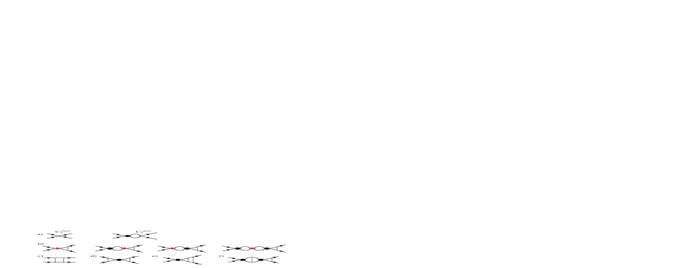
FIG. 2.: Order $Q$ diagrams for $\bar{\epsilon}_{1}$. The filled circle is defined in Fig. 1, and the diamonds in b) denote insertions of the ${}^{3}S_{1}-{}^{3}S_{1}$ operators with coefficients $C_{0}^{(0)}$, $C_{2}$ or $D_{2}$.

In dimensional regularization a graph with $k$ loops includes a factor of $(\mu_{R}/2)^{k(4-d)}$ (where the extra $2$ is inserted for convenience). Spin and isospin traces will be evaluated in $d-1$ dimensions for the reasons discussed in Appendix A. Of the graphs in Fig. 2 only e) and f) are divergent in $d=4-2\epsilon$ dimensions. The divergence in f) is cancelled by a graph with the NLO $\delta^{\rm uv}D_{2}$ counterterm given by Eq. (5.2) of Ref. [21]. The $p^{2}/\epsilon$ divergence in e) is cancelled by the new counterterm

$$\delta^{\rm uv}C_{2}^{(SD)}={3\sqrt{2}C_{0}^{\rm finite}\over 10}\Big{(}\frac{Mg_{A}^{2}}{8\pi f^{2}}\Big{)}^{2}\Big{(}\frac{1}{2\epsilon}-\gamma_{E}+\ln\pi\Big{)}\,.$$ (28)

Note that it is crucial to indicate what constants are subtracted along with the $1/\epsilon$ pole. The coupling $C_{2}^{(SD)}$ is determined from a fit to the observed $\bar{\epsilon}_{1}$. If the extracted value is to be used in other calculations, then its exact definition including finite subtractions will be needed. The divergence in Fig. 2 e) induces $\ln(\mu_{R})$ dependence in $C_{2}^{(SD)}(\mu_{R})$. In PDS

$$C_{2}^{(SD)}(\mu_{R})=\kappa C_{0}(\mu_{R})-{3\sqrt{2}\over 10}C_{0}(\mu_{R})\bigg{(}{Mg_{A}^{2}\over 8\pi f^{2}}\bigg{)}^{2}\ln\Big{(}{\mu_{R}^{2}\over\lambda^{2}}\Big{)}\,,$$ (29)

where $\kappa$ and $\lambda$ are constants. Note that there is only one unknown in Eq. (29) since a shift in the value of $\kappa$ can be compensated by changing the value of $\lambda$.

At order $Q$ the diagrams in Fig. 2 give the following amplitudes in the PDS scheme

$${\cal A}^{{SD}(1)}={\cal A}_{a}+{\cal A}_{b}+{\cal A}_{c}+{\cal A}_{d}+{\cal A}_{e}+{\cal A}_{f}\,,$$ (30)

where

$${i\cal A}_{a} = i\,C_{2}^{(SD)}\,p^{2}\bigg{[}1+\frac{M{\cal A}^{(-1)}}{4\pi}(ip+\mu_{R})\bigg{]}=-i\,{\cal A}^{(-1)}\,\frac{C_{2}^{(SD)}\,p^{2}}{C_{0}}\,,$$ (31)

$${i\cal A}_{b} = -i\,[{\cal A}^{(-1)}]^{2}\>\sqrt{2}\ \frac{(C_{2}\,p^{2}+D_{2}\,m_{\pi}^{2}+C_{0}^{(0)})}{C_{0}^{2}}\>\frac{m_{\pi}Mg_{A}^{2}}{8\pi f^{2}}\>{\cal X}(\alpha)\,,$$ (32)

$${i\cal A}_{c} = i{3\sqrt{2}\over 2}\ \frac{M}{4\pi}\Big{(}\frac{g_{A}^{2}}{2f^{2}}\Big{)}^{2}m_{\pi}\>{\cal Y}(\alpha)\,,$$ (33)

$${i\cal A}_{d} = -i\,{\cal A}^{(-1)}\sqrt{2}\ \Big{(}\frac{Mg_{A}^{2}}{8\pi f^{2}}\Big{)}^{2}\,m_{\pi}^{2}\bigg{[}i\alpha-\frac{i}{2\alpha}\ln(1-2i\alpha)\bigg{]}{\cal X}(\alpha)\,,$$ (34)

$${i\cal A}_{e} = i\,{\cal A}^{(-1)}\sqrt{2}\ \Big{(}\frac{Mg_{A}^{2}}{8\pi f^{2}}\Big{)}^{2}m_{\pi}^{2}\bigg{[}-\frac{3\alpha^{2}}{10}\ln\Big{(}\frac{\mu_{R}^{2}}{m_{\pi}^{2}}\Big{)}-i\,\alpha\,{\cal X}(\alpha)+{\cal Z}(\alpha)\bigg{]}\,,$$ (35)

$${i\cal A}_{f} = -i[{\cal A}^{(-1)}]^{2}\sqrt{2}\ \Big{(}\frac{M}{4\pi}\Big{)}^{3}\Big{(}\frac{g_{A}^{2}}{2f^{2}}\Big{)}^{2}m_{\pi}^{3}\bigg{[}(i\alpha)^{2}-\frac{\mu_{R}^{2}}{m_{\pi}^{2}}-\frac{1}{2}\ln\Big{(}\frac{\mu_{R}^{2}}{m_{\pi}^{2}}\Big{)}+\ln(1-2i\alpha)\bigg{]}{\cal X}(\alpha)\,.$$ (36)

The function ${\cal X}(\alpha)$ is given in Eq. (25), and the functions ${\cal Y}(\alpha)$ and ${\cal Z}(\alpha)$ are given in Appendix B. The sum of the amplitudes in Eq. (31) is:

$${\cal A}^{{SD}(1)} = -{\cal A}^{(-1)}\ \zeta_{6}\>\alpha^{2}-[{\cal A}^{(-1)}]^{2}\sqrt{2}\>\frac{m_{\pi}^{3}Mg_{A}^{2}}{8\pi f^{2}}\>{\cal X}(\alpha)\ (\zeta_{1}\alpha^{2}+\zeta_{2})$$ (39)

$$+\sqrt{2}\frac{Mm_{\pi}}{4\pi}\Big{(}\frac{g_{A}^{2}}{2f^{2}}\Big{)}^{2}\Bigg{\{}\frac{Mm_{\pi}{\cal A}^{(-1)}}{4\pi}\bigg{[}{\cal Z}(\alpha)+\frac{i}{2\alpha}\ln(1-2i\alpha){\cal X}(\alpha)\bigg{]}$$

$$\qquad\qquad\qquad\qquad\quad-\bigg{[}\frac{Mm_{\pi}{\cal A}^{(-1)}}{4\pi}\bigg{]}^{2}\ln(1-2i\alpha){\cal X}(\alpha)+{3\over 2}{\cal Y}(\alpha)+{\cal X}(\alpha)\Bigg{\}}\,,$$

where $\zeta_{1}$, $\zeta_{2}$, and $\zeta_{6}$ are $\mu_{R}$ independent dimensionless combinations of coupling constants:

$$\zeta_{1} = {C_{2}(\mu_{R})\over C_{0}(\mu_{R})^{2}}\,,\qquad\zeta_{2}={D_{2}(\mu_{R})\over C_{0}(\mu_{R})^{2}}+{C_{0}^{(0)}(\mu_{R})\over m_{\pi}^{2}C_{0}(\mu_{R})^{2}}-{g_{A}^{2}\over 2f^{2}}\bigg{(}\frac{M}{4\pi}\bigg{)}^{2}\bigg{[}\frac{1}{2}\ln\Big{(}\frac{\mu_{R}^{2}}{m_{\pi}^{2}}\Big{)}+{\mu_{R}^{2}-\gamma^{2}\over m_{\pi}^{2}}\bigg{]}\,,$$ (40)

$$\zeta_{6} = {m_{\pi}^{2}C_{2}^{(SD)}(\mu_{R})\over C_{0}(\mu_{R})}+{3\sqrt{2}\over 10}\bigg{(}{Mm_{\pi}g_{A}^{2}\over 8\pi f^{2}}\bigg{)}^{2}\ln\Big{(}{\mu_{R}^{2}\over m_{\pi}^{2}}\Big{)}\,.$$ (41)

$\zeta_{1}$ and $\zeta_{2}$ also appear in the NLO ${}^{3}S_{1}$ amplitude (see Eq. (A2)). $\zeta_{2}$ can be eliminated by imposing the condition that no spurious double pole should appear in this amplitude[16]:

$$\zeta_{2}={\gamma^{2}\over m_{\pi}^{2}}\zeta_{1}-{g_{A}^{2}\over 2f^{2}}\left(M\over 4\pi\right)^{2}{\rm log}\left(1~{}+{2\gamma\over m_{\pi}}\right).$$ (42)

The constant $\zeta_{1}$ is extracted from a fit to the ${}^{3}S_{1}$ phase shift at NLO. The order $Q$ contribution to $\bar{\epsilon}_{1}$ contains one unknown parameter, $\zeta_{6}$ or $C_{2}^{(SD)}(\mu_{R})$. This parameter is determined by fitting to the value of $\bar{\epsilon}_{1}$ from the Nijmegen partial wave analysis[26] at low momentum. Results for $\bar{\epsilon}_{1}$ are shown in Fig. 3. The solid line is the Nijmegen result. The order $Q$ result in the theory with pions [4] is shown by the dotted line. The result of the order $Q^{2}$ calculation in the theory with pions is given by the dot-dashed line in Fig. 3.

FIG. 3.: Predictions for the ${}^{3}S_{1}-{}^{3}D_{1}$ mixing parameter $\bar{\epsilon}_{1}$. The solid line is the multi-energy Nijmegen partial wave analysis [26]. The long and short dashed lines are the order $Q^{2}$ and $Q^{4}$ predictions in the theory without pions [14]. The dotted line is the order $Q$ prediction in the theory with pions from Ref. [4]. The dash-dotted line is the order $Q^{2}$ prediction in the theory with pions.

The values used in Fig. 3 are

$$\gamma=45.7\,{\rm MeV}\,,\qquad\zeta_{1}=0.2345\,,\qquad\zeta_{2}=-0.1038\,,\qquad\zeta_{6}=0.385\,.$$ (43)

The value of $\zeta_{6}$ in Eq. (43) corresponds to

$$C_{2}^{(SD)}(m_{\pi})=-4.56\>{\rm fm^{4}}\,.$$ (44)

For comparison results have also been shown in Fig. 3 for the theory without pions [14], where the prediction for $\bar{\epsilon}_{1}$ begins at order $Q^{2}$. The long dashed line is the order $Q^{2}$ result and the theory prediction has one free parameter. The short dashed line is the order $Q^{4}$ result which has two free parameters. With one less free parameter, the order $Q^{2}$ prediction of the theory with pions does better than the order $Q^{4}$ prediction of the theory without pions for $p>50\,{\rm MeV}$. In fact the theory without pions breaks down around $m_{\pi}/2$, as expected since this is where the pion cut begins. It has been noted in the literature [27] that many observables may not test the power counting for perturbative pions. As can be seen from Fig. 3, the mixing parameter provides an example in which perturbative pions clearly give improved agreement with the data.

The dot-dashed line in Fig. 3 improves over the order $Q$ result for $p<140\,{\rm MeV}$. For $p\sim m_{\pi}$, the error in the order $Q^{2}$ prediction for $\bar{\epsilon}_{1}$ is $\sim 20\%$. Recall that the mixing angle is small and an error of $\sim 0.5^{\circ}$ is consistent with our expectation for a NNLO calculation. It is interesting to ask how sensitive the results in Fig. 3 are to the choice of parameters. If we use the ${}^{3}S_{1}$ scattering length to fix $\gamma$ instead of the deuteron binding energy then the order $Q^{0}$ result (dotted line) increases by $\sim 1^{\circ}$ for $p\sim m_{\pi}$. Therefore, the mixing angle is quite sensitive to the location of the pole. On the other hand, the NNLO prediction is not sensitive to the value of $\zeta_{1}$ obtained from fitting the ${}^{3}S_{1}$ phase shift. This is because $\bar{\epsilon}_{1}^{(2)}$ in Eq. (23) depends on the linear combination

$$z=\zeta_{6}-0.56\,\zeta_{1}\,,$$ (45)

but is insensitive to the orthogonal combination. A change in $\zeta_{1}$ can be compensated by a change in $\zeta_{6}$ while keeping $z\simeq 0.255$. Solutions with the same $z$ give similar predictions, for instance, taking $\zeta_{1}=0.300$ and $\zeta_{6}=0.423$ gives an order $Q^{2}$ phase shift that differs by $<0.08^{\circ}$ from the one shown in Fig. 3.

A further test of the convergence of the $Q$ expansion is provided by examining the extent to which the amplitude violates unitarity. When Eq. (21) is expanded in powers of $Q$ the expression for $\bar{\epsilon}_{1}$ is explicitly real at each order in $Q$. However, one could insert the NLO expression for ${\cal A}^{SS}$ and ${\cal A}^{DD}$ and the NNLO expressions for ${\cal A}^{SD}$ into Eq. (21) and solve for $\bar{\epsilon}_{1}$ without making a $Q$ expansion. The resulting $\bar{\epsilon}_{1}$ will have an imaginary part which is order $Q^{3}$ in the power counting. Comparing the imaginary part of $\bar{\epsilon}_{1}$ calculated using Eq. (21) to $\bar{\epsilon}_{1}^{(1)}+\bar{\epsilon}_{1}^{(2)}$ gives $|{\rm Im}(\bar{\epsilon}_{1})/(\bar{\epsilon}_{1}^{(1)}+\bar{\epsilon}_{1}^{(2)})|\leq 0.2$ for $p\leq 180\,{\rm MeV}$, which is of the expected size for an order $Q^{2}$ quantity. Also, for $p\leq m_{\pi}$ the ratio $|{\cal A}^{SD(1)}/{\cal A}^{SD(0)}|\leq 0.6$, which is consistent with an expansion parameter of order $1/2$. The agreement of the size of these terms with our expectations suggests that the $Q$ expansion is under control.

FIG. 4.: Prediction for $\bar{\epsilon}_{1}$ from Ref. [2]. The fit was done to the partial wave analysis in Ref. [26] shown by the solid line. The long dashed line uses the cutoff $\Lambda=0.6\,m_{\rho}$, the short dashed line uses $\Lambda=m_{\rho}$, and the dotted line uses $\Lambda=1.3\,m_{\rho}$.

In Ref. [2], the mixing angle is calculated using Weinberg’s power counting. In this approach, momentum power counting is applied to the potential and then the Schroedinger equation is solved numerically. Solving the Schroedinger equation with the one pion exchange potential is equivalent to summing ladder graphs with potential pion exchange to all orders. However, all necessary counterterms are not included, so there is a residual dependence on the cutoff. This cutoff dependence can be used to give an estimate of the uncertainty in the theoretical prediction due to higher order effects. We will compare our calculation with that of Ref. [2], however it is important to keep in mind that Ref. [2] includes graphs which are higher order in $Q$ than those in Fig. 2. Ref. [2] also includes $\Delta$’s and more parameters are varied in the fit. The results of Ref.[2] are shown in Fig. 4. Varying the cutoff between $0.6\,m_{\rho}$ and $1.3\,m_{\rho}$ gives an uncertainty of $0.7^{\circ}$ at $p=m_{\pi}$. This uncertainty is comparable to the error in our fit which differs from the data by $0.5^{\circ}$ at $p=m_{\pi}$. The error in our calculation increases for larger values of $p$ because our prediction grows with $p$ faster than the observed $\bar{\epsilon}_{1}$. For these values of $p$ the nonperturbative calculation suffers from considerable uncertainty. For a cutoff equal to $m_{\rho}$, the prediction grows with $p$, but with a lower value of the cutoff ($0.6\,m_{\rho}$) the calculated $\bar{\epsilon}_{1}$ provides better agreement with data. It would be interesting to work to one higher order in $Q$ and/or include $\Delta$’s with the KSW power counting to see if the agreement with data at higher $p$ improves. At one higher order in $Q$ a four derivative four nucleon ${}^{3}S_{1}-{}^{3}D_{1}$ operator appears. However, using the renormalization group its coefficient is determined in terms of $C_{0}$, $C_{2}$, and $C_{2}^{(SD)}$.

For momenta $p\ll m_{\pi}$, effective range expansions can be constructed for the phase shifts and mixing angle. By integrating the pion out of the effective field theory coefficients in this expansion can be predicted. In Ref. [28] coefficients in the expansions of $p\,\cot\delta^{(^{1}S_{0})}$, $p\,\cot\bar{\delta}_{0}$, and $\bar{\epsilon}_{1}$ are obtained from the order $Q^{0}$ calculations in Ref. [4]. Ref. [28] found that the effective field theory gives parameter free predictions for the higher coefficients, but these did not agree with fits [29] to the partial wave data. However, it is not clear whether the extraction of higher order terms in the expansion is accurate enough to test the effective field theory [20]. In toy models it has been shown that the convergence of the effective field theory predictions for these coefficients is slow[30]. This also seems to be the case when the effective field theory is applied to real data. In Ref. [16] it was found that the order $Q$ corrections to the coefficients of $p\,\cot\delta^{(^{1}S_{0})}$ improve the agreement with the fit values, however the observed convergence is rather slow.

From the amplitude in Eq. (39) the order $Q^{2}$ corrections to the momentum expansion of $\bar{\epsilon}_{1}$ can be derived. The expansion in the theory without pions takes the form [14]

$$\bar{\epsilon}_{1}=b_{1}{p^{3}\over\sqrt{p^{2}+\gamma^{2}}}+b_{2}{p^{5}\over\sqrt{p^{2}+\gamma^{2}}}+\ldots\,,$$ (46)

where $b_{1}$ and $b_{2}$ are constants. $\bar{\epsilon}_{1}$ has a cut at $p=\pm i\gamma$, so the momentum expansion of $\bar{\epsilon}_{1}$ only converges for $p<\gamma$. Clearly it would be more useful to expand a function with better analyticity properties. Following Ref. [31] this can be done by parameterizing the S-matrix as:

$$S=\left(\begin{array}[]{cc}\cos\epsilon_{1}&-\sin\epsilon_{1}\\ \sin\epsilon_{1}&\cos\epsilon_{1}\end{array}\right)\left(\begin{array}[]{cc}e^{2i\delta_{0}}&0\\ 0&e^{2i\delta_{2}}\end{array}\right)\left(\begin{array}[]{cc}\cos\epsilon_{1}&\sin\epsilon_{1}\\ -\sin\epsilon_{1}&\cos\epsilon_{1}\end{array}\right)\,.$$ (53)

$p\cot\delta_{0},\,$ $p^{5}\cot\delta_{2},\,$ and $\epsilon_{1}$ have momentum expansions with radius of convergence $m_{\pi}/2$ rather than $\gamma$. For low energy expansions these variables should be used. The expressions for $\delta_{0,2}$ and $\bar{\delta}_{0,2}$ are the same to order $Q$. The mixing angle in this parameterization is related to the one in Eq. (20) by

$$\tan(2\,\epsilon_{1})={\tan(2\,\bar{\epsilon}_{1})\over\sin(\bar{\delta}_{0}-\bar{\delta}_{2})}={2{\cal A}^{SD}\over{\cal A}^{SS}-{\cal A}^{DD}}\,.$$ (54)

In terms of the amplitudes, the first two terms in the $Q$ expansion of $\epsilon_{1}$ are

$$\epsilon_{1}^{(1)} = {{\cal A}^{SD(0)}\over{\cal A}^{(-1)}}\,,\qquad\epsilon_{1}^{(2)}={\rm Re}\bigg{[}\frac{{\cal A}^{{SD}(1)}}{{\cal A}^{(-1)}}\bigg{]}-\frac{M\gamma}{4\pi}\>\epsilon_{1}^{(1)}\>\bigg{[}{\cal A}^{DD(0)}-|{\cal A}^{(-1)}|^{2}{{\cal A}^{SS(0)}\over({\cal A}^{(-1)})^{2}}\bigg{]}\ \,.$$ (55)

FIG. 5.: Predictions for the mixing parameter $\epsilon_{1}$ defined in Eq. (53). The solid line is the multi-energy Nijmegen partial wave analysis [26]. The dotted line is the NLO prediction in the theory with pions from Ref. [4]. The dash-dotted line is the NNLO prediction in the theory with pions. The open circles are data from Virginia Tech [32] and the stars are Nijmegen single energy data [26] whose quoted errors are invisible on the scale shown.

In Fig. 5 we plot the order $Q$ and $Q^{2}$ effective field theory predictions for $\epsilon_{1}$ using the parameters in Eq. (43). The open circles in Fig. 3 are data from Virginia Tech [32]. The stars are the Nijmegen single energy fit to the data [26] whose quoted errors are invisible on the scale shown. It seems somewhat strange that the data point at $p=265\,{\rm MeV}$ from Ref. [32] differs from the fit in Ref. [26] by more than eight standard deviations.

$\epsilon_{1}$ has a series expansion in $p^{2}$:

$$\epsilon_{1} = g_{1}\,p^{2}+g_{2}\,p^{4}+g_{3}\,p^{6}+\ldots\,.$$ (56)

Fitting this polynomial to the solid line in Fig. 5 for $7\,{\rm MeV}<p<50\,{\rm MeV}$ and weighting low momenta more heavily than high momenta gives the values in the first column in Table I. To estimate the uncertainty in the extraction of the $g_{i}$ we varied the range of momentum and weighting used in the fit. The value of $g_{1}$ is quite stable, while $g_{2}$ and $g_{3}$ varied by 10% and 50% respectively. The effective field theory predictions for the coefficients $g_{i}$ are:

$$g_{1} = \frac{2\sqrt{2}}{m_{\pi}\Lambda_{NN}}\bigg{(}\frac{8}{15}-\frac{\gamma}{m_{\pi}}\bigg{)}-\frac{\sqrt{2}}{\Lambda_{NN}^{2}}\bigg{(}\frac{601}{600}-\frac{8}{5}\ln 2-\frac{5\,\gamma}{m_{\pi}}+\frac{2\,\gamma^{2}}{m_{\pi}^{2}}\bigg{)}-\frac{\zeta_{6}}{m_{\pi}^{2}}+\frac{8\pi\,\sqrt{2}\,\zeta_{2}}{M\,\Lambda_{NN}}\,,$$ (57)

$$g_{2} = \frac{4\sqrt{2}}{m_{\pi}^{3}\Lambda_{NN}}\bigg{(}\frac{-32}{35}+\frac{5\,\gamma}{3\,m_{\pi}}\bigg{)}+\frac{4\sqrt{2}}{m_{\pi}^{2}\Lambda_{NN}^{2}}\bigg{(}\frac{391}{315}-\frac{4}{5}\ln 2-\frac{589\,\gamma}{120\,m_{\pi}}+\frac{8\,\gamma^{2}}{3\,m_{\pi}^{2}}\bigg{)}$$ (59)

$$+\frac{2\sqrt{2}}{m_{\pi}^{2}\Lambda_{NN}}\,\frac{4\pi}{M}\Big{(}\zeta_{1}-\frac{10}{3}\zeta_{2}\Big{)}\,,$$

$$g_{3} = \frac{16\sqrt{2}}{m_{\pi}^{5}\Lambda_{NN}}\bigg{(}\frac{16}{21}-\frac{7\,\gamma}{5\,m_{\pi}}\bigg{)}-\frac{16\sqrt{2}}{m_{\pi}^{4}\Lambda_{NN}^{2}}\bigg{(}\frac{241}{200}-\frac{3}{5}\ln 2-\frac{252409\,\gamma}{50400\,m_{\pi}}+\frac{46\,\gamma^{2}}{15\,m_{\pi}^{2}}\bigg{)}$$ (61)

$$-\frac{8\sqrt{2}}{m_{\pi}^{4}\Lambda_{NN}}\,\frac{4\pi}{M}\Big{(}\frac{5}{6}\zeta_{1}-\frac{14}{5}\zeta_{2}\Big{)}\,.$$

In each $g_{i}$ the first term is from the order $Q^{0}$ diagrams in Fig. 1, while the remaining terms are from the order $Q$ diagrams in Fig. 2. Using the values in Eq. (43) gives the predictions in Table. I. At order $Q^{0}$ the effective field theory is off by a factor of $2$. The order $Q$ corrections make the predictions closer to the fit values; the error is $\sim 25\%$ for $g_{1}$ and $g_{2}$, while $g_{3}$ is consistent within error. The effective field theory is converging onto the experimental $g_{i}$, but the errors are somewhat larger than anticipated by the power counting. The convergence for terms in the expansion of $\epsilon_{1}$ is faster than the convergence in the ${}^{1}S_{0}$ channel.

		Fit to Nijmegen $\epsilon_{1}$	${\cal O}(Q^{0})$	${\cal O}(Q)$
	$g_{1}\,(\rm fm^{2})$	$\>0.30\pm 0.01$	$0.55$	$0.22$
	$g_{2}\,(\rm fm^{4})$	$-2.0\pm 0.2$	$-4.1$	$-1.5$
	$g_{3}\,(\rm fm^{6})$	$\>8.7\pm 4.3$	$28$	$9.5$

TABLE I.: Predictions for the coefficients in a momentum expansion of $\epsilon_{1}$ at LO and NLO in the effective field theory.

To summarize, we have computed the order $Q^{2}$ correction to the mixing parameter ${\epsilon}_{1}$. The effective theory converges onto the observed ${\epsilon}_{1}$, and errors are comparable to uncertainties in alternative approaches where the pion is treated nonperturbatively for $p\sim m_{\pi}$. When performing low energy momentum expansions, it is important to use a parameterization of the S matrix in which the mixing angle has a convergent expansion for $p<m_{\pi}/2$. The effective field theory predictions for the coefficients of this expansion converge towards values extracted from a fit to low energy data. In the future, it will be interesting to see if including the $\Delta$ or going to one higher order in the $Q$ expansion will provide better agreement for $\epsilon_{1}$ at $p>m_{\pi}$.

S.F. was supported in part by NSERC and wishes to thank the Caltech theory group for their hospitality. T.M and I.W.S. were supported in part by the Department of Energy under grant number DE-FG03-92-ER 40701.

Note Added in Proof: While this paper was being reviewed, the authors completed a NNLO calculation of the phase shifts in the ${}^{1}S_{0}$, ${}^{3}S_{1}$, and ${}^{3}D_{1}$ channels. Predictions for the other P and D wave phase shifts were also examined. We find that in some of these channels the KSW expansion exhibits large corrections at NNLO which suggest a breakdown of the perturbative treatment of pions. A detailed discussion can be found in the preprint [24].

A Traces in $n$ Dimensions

In the standard implementation of dimensional regularization in relativistic theories, the spin traces are performed in $d$ dimensions [34]. For non-relativistic nucleon-nucleon scattering the spin traces are often done in $3$ dimensions, after which the remaining scalar integrals are evaluated in $d=n+1$ dimensions. This is in agreement with performing a partial wave expansion of the matrix elements using Clebsh-Gordan coefficients; a procedure specific to $n=3$. This approach provides well-defined results for S-wave transitions. However, when higher partial waves are considered it becomes necessary to perform the spin traces in $n$ dimensions. To see why consider Fig. 2 e), and replace the bubble sum by a single $C_{0}$ for simplicity. The numerator of this graph is proportional to

$$\Big{(}\frac{p^{i}p^{i^{\prime}}}{p^{2}}-\frac{\delta^{ii^{\prime}}}{n}\Big{)}{\rm Tr}[\sigma^{i}\sigma^{j}\sigma^{m}\sigma^{i^{\prime}}\sigma^{m^{\prime}}\sigma^{j^{\prime}}]\,q^{m}\,q^{m^{\prime}}\,k^{j}\,k^{j^{\prime}}\,,$$ (A1)

where $k$ and $q$ are the two loop momenta which run through the pion lines. First consider setting $\delta^{ii^{\prime}}/n=\delta^{ii^{\prime}}/3$ in Eq. (A1) and performing the trace in $4$ dimensions. At very low momentum, the result can be expanded in $p/m_{\pi}$. When this is done, the amplitude from this graph is proportional to a constant for low $p$. However, for a ${}^{3}S_{1}$ to ${}^{3}D_{1}$ transition the amplitude should be proportional to $p^{2}$ at low momentum. The constant indicates that projection onto ${}^{3}S_{1}-{}^{3}D_{1}$ was unsuccessful. If we keep the $\delta^{ii^{\prime}}/n$ in Eq. (A1), and perform the trace in $3$ dimensions then the amplitude is still proportional to a constant for low momentum. However, if the trace in Eq. (A1) is done in $n$ dimensions then the amplitude is proportional to $p^{2}$ as it should be. In the ${}^{3}S_{1}-{}^{3}D_{1}$ calculation the two terms in round brackets in Eq. (A1) have $m_{\pi}^{2}/\epsilon$ divergences. These divergences cancel in the difference no matter how the expression is evaluated, because there is no operator in this partial wave to absorb an $m_{\pi}^{2}/\epsilon$ divergence. However, the finite $m_{\pi}^{2}$ contributions only cancel when spin traces and projection operators are evaluated in $n$ dimensions. Therefore, in this paper all spin traces will be performed in $n$ dimensions.

In Ref. [19, 33] it was pointed out that the nucleon contact interactions with no derivatives are invariant under Wigner’s SU(4) spin-isospin symmetry for $a^{(^{1}S_{0})},a^{(^{3}S_{1})}\to\infty$. If spin traces are performed in $n$ dimensions then it is necessary to treat the isospin traces on the same footing, otherwise Wigner symmetry will be broken by the regulator. For this reason, isospin traces will also be done in $n$ dimensions. For example, if the order $Q_{r}^{3}$ radiation pion calculation in Ref. [25] is performed with spin traces in $n$ dimensions, but isospin traces in $3$ dimensions then the result is not proportional to $1/a(^{1}S_{0})-1/a(^{3}S_{1})$. However, in Ref. [19] it was shown that Wigner symmetry implies that the order $Q_{r}^{3}$ graphs should be proportional to $1/a(^{1}S_{0})-1/a(^{3}S_{1})$. If all spin and isospin traces are performed in $n$ dimensions then the value of individual order $Q_{r}^{3}$ graphs changes, but the sum gives the same result as in Ref. [25].

If the partial wave projection operators are chosen to have the normalization given in Eq. (7) then doing the traces in $n$ dimensions does not change any calculations in the theory without pions. For S-wave transitions in the theory with pions this convention amounts to a change of renormalization scheme, since the difference in evaluating a graph is an overall multiplicative factor of the form $1+O(\epsilon)$. In PDS, subleading terms in the beta functions for coefficients of four nucleon operators are affected. When spin and isospin traces are done in $n$ dimensions the NLO ${}^{3}S_{1}$ (or ${}^{1}S_{0}$) amplitude is

$${{\cal A}^{(0)}\over[{\cal A}^{(-1)}]\,^{2}} = -m_{\pi}^{2}(\zeta_{1}\,\alpha^{2}+\zeta_{2})+{m_{\pi}^{2}g_{A}^{2}\over 2f^{2}}\bigg{(}\frac{M}{4\pi}\bigg{)}^{2}\Bigg{[}{(\hat{\gamma}^{2}-\alpha^{2})\over 4\alpha^{2}}\ln(1+4\alpha^{2})-{\hat{\gamma}\over\alpha}\tan^{-1}(2\alpha)\Bigg{]}\,,$$ (A2)

where $\hat{\gamma}=\gamma/m_{\pi}$ and $\zeta_{1}$ and $\zeta_{2}$ are given in Eq. (40). Different schemes will give different expressions for $\zeta_{1,2}$, but the amplitude in Eq. (A2) will remain the same.

B Expressions for ${\cal Y}$ and ${\cal Z}$

In this appendix we give expressions for ${\cal Y}$ and ${\cal Z}$ which appear in Eqs. (31) and (39):

$${\cal Y}(\alpha) = -\frac{2}{5}+\frac{3}{10\alpha^{2}}+\bigg{(}\frac{3}{8\alpha^{5}}+\frac{5}{4\alpha^{3}}-\frac{2\alpha}{5}\bigg{)}\tan^{-1}(\alpha)-\bigg{(}\frac{3}{8\alpha^{5}}+\frac{5}{4\alpha^{3}}\bigg{)}\tan^{-1}(2\alpha)$$ (B3)

$$+\frac{(15-4\alpha^{2})}{80\alpha^{6}}\ln(1+\alpha^{2})-\frac{(3+16\alpha^{2}+16\alpha^{4})}{32\alpha^{7}}{\rm Im}\,\bigg{[}{\rm Li}_{2}\Big{(}\frac{2\alpha^{2}+i\alpha}{1+4\alpha^{2}}\Big{)}+{\rm Li}_{2}(-2\alpha^{2}-i\alpha)\bigg{]}$$

$$+i\bigg{[}\frac{3}{8\alpha^{3}}+\frac{1}{2\alpha}-\frac{\alpha}{2}-\frac{(3+10\alpha^{2})}{16\alpha^{5}}\ln(1+4\alpha^{2})+\frac{(3+16\alpha^{2}+16\alpha^{4})}{128\alpha^{7}}\ln^{2}(1+4\alpha^{2})\bigg{]}\,,$$

$${\cal Z}(\alpha) = -\frac{7}{40}+\frac{9i}{16\alpha^{3}}+\frac{21}{40\alpha^{2}}+\frac{3i}{40\alpha}-\frac{3i\alpha}{5}+\frac{29\alpha^{2}}{200}+\Big{(}\frac{3\alpha^{2}}{5}-\frac{9}{16\alpha^{4}}-\frac{15}{8\alpha^{2}}\Big{)}\ln{2}$$ (B7)

$$+\frac{3\,(16\alpha^{7}-50\alpha^{3}-4i\alpha^{2}-15\alpha+15i)}{80\alpha^{5}}\ln(1-i\alpha)$$

$$+\frac{(-9\,i+27\,\alpha-24\,i\,{{\alpha}^{2}}+78\,{{\alpha}^{3}}-16\,{{\alpha}^{5}})}{32\alpha^{5}}\ln(1-2i\alpha)$$

$$-\frac{(9+48\alpha^{2}+48\alpha^{4})}{64\alpha^{6}}\bigg{[}\frac{3}{2}\ln^{2}(1-2i\alpha)+2{\rm Li}_{2}(-1+2i\alpha)+{\rm Li}_{2}\Big{(}\frac{1+2i\alpha}{-1+2i\alpha}\Big{)}+\frac{\pi^{2}}{4}\bigg{]}\,.$$

In deriving the formula for ${\cal Z}(\alpha)$ we found it useful to use reduction formulae due to Tarasov[35] implemented with the program from Ref. [36].

REFERENCES

[1] S. Weinberg, Phys. Lett. B251 (1990) 288; Nucl. Phys. B363 (1991) 3; C. Ordonez and U. van Kolck, Phys. Lett. B291 (1992) 459; C.
Ordonez, L. Ray and U. van Kolck, Phys. Rev. Lett. 72 (1994) 1982; U. van Kolck,
Phys. Rev. C49 (1994) 2932; G.P. Lepage, nucl-th/9706029,
[2]
C. Ordonez, L. Ray, and U. van Kolck,
Phys. Rev. C53, (1996) 2086,
[3]
D. B. Kaplan, M. J. Savage, and M. B. Wise,
Phys. Lett. B424 (1998) 390,
[4]
D. B. Kaplan, M. J. Savage, and M. B. Wise,
Nucl. Phys. B534 (1998) 329,
[5]
E. Epelbaum and U.-G. Meissner, nucl-th/9903046,
[6]
X. Kong and F. Ravndal, hep-ph/9903523;
Phys. Lett. B450, (1999) 320,
[7]
X. Kong and F. Ravndal, nucl-th/9902064;
nucl-th/9904066,
[8] D. B. Kaplan, M. J. Savage, and M. B. Wise, Phys. Rev. C59
(1999) 617,
[10] M. J. Savage, K. A. Scaldeferri, and M. B. Wise, nucl-th/9811029;
J.-W. Chen, G. Rupak, and M. J. Savage, nucl-th/9905002,
[11] J.-W. Chen, H. W. Griesshammer, M. J. Savage, and R. P. Springer,
Nucl. Phys. A644, 245 (1998);
J.-W. Chen, nucl-th/9810021,
[12] D. B. Kaplan, M. J. Savage, R. P. Springer, and M. B. Wise,
Phys. Lett. B449, (1999) 1;
M. J. Savage and R. P. Springer, Nucl. Phys. A644 (1998) 235,
[13] Malcolm Butler and Jiunn-Wei Chen, nucl-th/9905060.
[14] J.-W. Chen, G. Rupak, and M. J. Savage, nucl-th/9902056,
[15] G. Rupak and N. Shoresh, nucl-th/9902077,
[16] T. Mehen and I. W. Stewart, nucl-th/9906010,
[17] M. Binger, nucl-th/9901012,
[18] E. Wigner, Phys. Rev. 51, 106, 947 (1937).
[19] T. Mehen, I. W. Stewart, and M. B. Wise, hep-ph/9902370,
[20] T. Mehen and I. W. Stewart, Phys. Lett. B445, (1999) 378,
[21] T. Mehen and I. W. Stewart, Phys. Rev. C59 (1999) 2365,
[22] U. van Kolck, hep-ph/9711222,
[23] H.P. Stapp, T.J. Ypsilantis, and N. Metropolis, Phys. Rev. 105
(1957) 302,
[24] S. Fleming, T. Mehen, and I.W. Stewart, nucl-th/9911001,
[25] T. Mehen and I. W. Stewart, nucl-th/9901064,
[26] V. G. J. Stoks, et. al.,
Phys. Rev. C48, 792 (1993),
http://nn-online.sci.kun.nl/NN/,
[27] T. D. Cohen and J. M. Hansen, nucl-th/9901065,
[28] T. D. Cohen and J. M. Hansen, nucl-th/9808038,
[32]
R.A. Arndt and R. L. Workman, Few Body Syst. Suppl. 7, 64 (1994);
R.A. Arndt, J.S. Hyslop, III, and L.D. Roper, Phys. Rev. D35, 128 (1987);
R.A. Arndt and L.D. Roper, Scattering Analysis Interactive Dial-in Program (SAID),
http://said.phys.vt.edu/,
[33] P.F. Bedaque, H.-W. Hammer, and U. van Kolck, nucl-th/9906032,
[34] J. Collins,
Renormalization (Cambridge University
Press, Cambridge, 1984).