Effective field theory for nuclear matter

Abstract

We apply the relativistic chiral Lagrangian to the nuclear equation of state. An effective chiral power expansion scheme, which is constructed to work around nuclear saturation density, is presented. The leading and subleading terms are evaluated and are shown to provide an equation of state with excellent saturation properties. Our saturation mechanism is found to probe details of the nuclear pion dynamics.

1 Introduction

The nuclear equation of state awaits a fundamental theoretical description. It is therefore important to develop the appropriate form of effective chiral perturbation theory (E$\chi$PT), a promising tool of modern nuclear physics, and apply it to the nuclear many body problem systematically.

The key element of any microscopic theory for the nuclear equation of state is the elementary nucleon-nucleon scattering process. In the context of chiral perturbation theory this problem was first addressed by Weinberg who proposed to derive a chiral nucleon-nucleon potential in time ordered perturbation theory [1, 2]. In [3, 4] we proposed an alternative scheme with chiral power counting rules applied directly to the nucleon-nucleon scattering amplitude. This approach applies the manifest covariant version of the chiral Lagrangian and relies on the crucial observation that the chiral power counting rules can be generalized for 2-nucleon reducible diagrams. Non-perturbative effects like the pseudo bound state pole in the ${}^{1}S_{0}$ channel are generated by properly renormalized local two-nucleon vertices. A similar approach was suggested by Kaplan, Savage and Wise [5] in the context of the chiral potential approach. Unfortunately the straightforward application of the extended counting rules to the s-wave nucleon-nucleon scattering phase shifts is hampered by a poor convergence and inconsistency with empirical data[6]. In particular, unitarity is violated strongly even at small energy where one would expect this scheme to work well[4]. This is, at first glance, a surprising result since it is long known that for the one pion exchange Yukawa potential perturbation theory works fine if the coupling strength is put to its empirical value[7, 8, 9]. In fact in the ${}^{1}S_{0}$ channel, the failure of a naive expansion is linked to the presence of a second strong subthreshold singularity reflecting a subtle interplay of intermediate attraction and short range repulsion[4]. A properly modified unitary implementation of the extended chiral counting rules describes empirical s-wave elastic and inelastic nucleon-nucleon scattering in the spin singlet channel accurately up to $E_{\rm lab}\simeq 600$ MeV[4].

We point out that counting rules for the vacuum nucleon-nucleon scattering amplitude greatly facilitate the construction of chiral power counting rules for the nuclear matter problem[10]. Basically the density expansion or equivalently the multiple scattering expansion can be combined smoothly with the chiral expansion where one identifies $k_{F}\sim Q$ as a further small scale. Such an identification leads to a systematic resummation of the density expansion avoiding the expansion in large ratios like $k_{F}/m_{\pi}$ but exploiting the chiral mass gap and expand in small ratios like $k_{F}/m_{\chi}$ or $m_{\pi}/m_{\chi}$ with $m_{\chi}\simeq m_{N}$.

2 Primer on relativistic chiral nucleon-nucleon scattering

In this section we recall basic elements required for a successful application of the relativistic chiral Lagrangian to the baryon sector. The systematic construction of the Lagrangian density in accordance with chiral symmetry was presented in great detail by Weinberg using stereographic coordinates [11]. There are two problems when evaluating the relativistic chiral Lagrangian in the baryon sector. First, any covariant derivative acting on the nucleon field produces the large nucleon mass and therefore must be assigned the minimal chiral power zero. Thus an infinite tower of interaction terms needs to be evaluated at given finite chiral order [12, 13]. Second, the straightforward evaluation of relativistic diagrams involving nucleon propagators generates positive powers of the large nucleon mass from loop momenta larger than the nucleon mass. The chiral power counting rules are spoiled. The relativistic scheme appeared impractical and the heavy mass formulation of $\chi$PT, which overcomes both problems by performing a non relativistic $1/m$ expansion at the level of the Lagrangian density, was developed [14] and applied extensively in the one-nucleon sector [15].

We point out that in the two-nucleon channel it will be advantageous to work with the relativistic form of the chiral Lagrangian [3, 4]. One reason is that in the heavy baryon formulation two-particle reducible diagrams are ill defined. A second reason is that a proper treatment of the pion production process $pp\rightarrow pp\,\pi^{0}$ requires relativistic kinematics[4]. Note that an alternative scheme to tame potentially ill defined two-particle reducible diagrams is the use of time-ordered perturbation theory as suggested by Weinberg[1]. Since covariance is not manifest in time-ordered perturbation theory we prefer the relativistic scheme. Here we outline how the two aforementioned problems can be overcome within the framework of the relativistic chiral Lagrangian. Of course we expect the relativistic scheme to be equivalent to the more familiar heavy fermion formulation of chiral perturbation theory in the one-nucleon sector. Rather than performing the $1/m$ expansion at the level of the Lagrangian density we suggest to work out this expansion explicitly at the level of individual relativistic Feynman diagrams. Therewith we avoid the heavy baryon chiral Lagrangian with its known artifacts in the two-nucleon sector. Here it is convenient to consider the chiral Lagrangian (at an intermediate stage) to represent a finite cutoff theory. The finite cutoff, $\Lambda\ll m$, is required to restrict the nucleon virtuality inside a given loop diagram such as to justify the $1/m$ expansion. Obviously a finite cutoff has to be introduced with great care not to break any chiral Ward identity. Note that one may alternatively apply dimensional regularization. We emphasize that obviously if dimensional regularization is applied one has to first expand in $1/m$ and then perform the loop integration. The two steps do not commute here.

We need to outline how to arrange higher order terms of the relativistic chiral Lagrangian in the nucleon sector. To have a practical scheme one would like to have only a finite number of interaction terms with a given number of ’small’ derivatives involved. The known problem of the ’large’ nucleon mass generated by time derivatives acting on a nucleon field has to be taken care of. This problem is cured easily as follows. Consider a covariant derivative ${\mathcal{D}}_{\mu}(x)$ acting on a nucleon field $N(x)$. We need to construct a ’counter interaction’ which leads to a small renormalized vertex. This rearrangement is illustrated at hand of the simple case when the Lorentz index $\mu$ is saturated by another covariant derivative acting on the same nucleon field. In this case the counter interaction is readily found

$${\mathcal{D}}^{\mu}(x)\,{\mathcal{D}}_{\mu}(x)\,N(x) \rightarrow\left({\mathcal{D}}^{\mu}(x)\,{\mathcal{D}}_{\mu}(x)+m^{2}\right)\,N(x)$$ (1)

$$\rightarrow-\left(p^{2}-m^{2}\right)\sim Q$$

and the ’renormalized’ vertex is proportional to the virtuality of the nucleon 4-momentum which is of ’minimal’ order $Q$. It is important to observe that this counter interaction must have occurred already in the chiral Lagrangian to some lower order since it involves fewer derivatives. Note that a similar construction works if two covariant derivatives act on different nucleon fields.

We are left to consider the case in which the Lorentz index $\mu$ of the covariant derivative ${\mathcal{D}}_{\mu}$ is contracted either with the Lorentz index of a Dirac matrix or the Lorentz index of a derivative acting on a pion field. Interaction vertices in which a covariant nucleon derivative ${\mathcal{D}}_{\mu}$ is saturated with a pionic four vector $D^{\mu}$ or with the Lorentz index of its covariant derivative behave well since they are already suppressed by the small derivative acting on the pion field. Here one has to assign the nucleon derivative the chiral power $Q^{0}$. The large nucleon mass present is not hazardous provided that one may identify the natural scale $\bar{\Lambda}$ of chiral interactions with the nucleon mass. With $\bar{\Lambda}\simeq m_{\rho}$ this seems indeed reasonable. The remaining case in which the nucleon derivative couples to the Lorentz index of a Dirac matrix does not generate an infinite tower of interaction terms since at a given number of nucleon fields, $n_{i}$, the number of available Lorentz indices provided by Dirac matrices is at most $n_{i}$.

The above arguments show how to organize the infinite tower of chiral interaction terms such that there is always only a finite number of terms with a given number of ’small’ derivatives. Thus at any given chiral order only a finite number of diagrams need to be evaluated. The result of this reorganization of the relativistic chiral Lagrangian leads to the applicability of Weinberg’s counting rules provided that individual diagrams are expanded properly.

In the two-nucleon sector the chiral Lagrangian leads to a well defined expansion scheme for the Bethe-Salpeter kernel K. For the unitary iteration of K, as induced by the Bethe-Salpeter equation, Weinberg’s counting rules are not applicable due to the s-channel unitarity cut. Nevertheless a generalized counting for two-particle reducible diagrams can be established. For a given diagram each pair of intermediate nucleons causes a reduction of one chiral power as compared to the ’naive’ chiral power [3]. The argument goes as follows: consider the once iterated Bethe-Salpeter kernel

$$K\,G\,K\sim\int\frac{d^{4}l}{(2\pi)^{4}}\frac{2\,m\,K(l)}{\Big{(}{\textstyle{1\over 2}}\,W-l\Big{)}^{2}-m^{2}+i\,\epsilon}\frac{2\,m\,K(l)}{\Big{(}{\textstyle{1\over 2}}\,W+l\Big{)}^{2}-m^{2}+i\,\epsilon}$$ (2)

with $W^{2}=s$. The object $G$ represents the two-nucleon propagator and $K$ the Bethe-Salpeter kernel evaluated according to Weinberg’s counting rules to a given chiral order. It is instructive first to study the s-channel spectral density, $\rho(s)$, of this contribution. Since by assumption the Bethe-Salpeter kernel $K$ is 2-nucleon irreducible the s-channel spectral density picks up strength only from the pinch singularity generated by the two nucleon propagators in (2). In the center of mass frame with $\vec{W}=0$ one finds:

$$\rho(s)=\Im\,K\,G\,K\sim\frac{p}{\sqrt{m^{2}+p^{2}}}\,\frac{m^{2}}{4\,\pi}\,\int\,\frac{d\Omega_{\vec{l}}}{4\,\pi}\,K(\vec{l}\,)\,K(\vec{l}\,)\,\Big{|}_{l_{0}=0,\,|\vec{l}|=p}$$ (3)

with $s=4\left(m^{2}+p^{2}\right)$. Expression (3) can now be used to introduce the chiral power, $\nu$, of the s-channel spectral density, $\rho(s)$,

$$\nu=1+2\,\nu_{K}$$ (4)

with the chiral power $\nu_{K}$ of the Bethe-Salpeter kernel $K$ as given by Weinberg’s power counting rules. In (4) we exploit the important observation that the small scale momentum $p\sim Q$ occurs in the spectral density.

To have a useful scheme we also need to derive counting rules for the real part of the scattering amplitude. Here we evoke causality which relates the real part of a given Feynman diagram to its imaginary part by means of a dispersion relation

$$I(s)=\Re K\,G\,K=\frac{1}{\pi}\,{\mathcal{P}}\int_{4\,m^{2}}^{\infty}d\,\bar{s}\,\frac{\rho(\bar{s})}{\bar{s}-s-i\,\epsilon}\;.$$ (5)

Of course we must not assume the dispersion relation (5) to be finite and well defined. It may be ultraviolet divergent. However, we recall that we are free to consider our chiral Lagrangian as a finite cutoff theory. So let us introduce a covariant cutoff $\Lambda$ into the dispersion relation (5). If the cutoff $\Lambda$ is to be interpreted as a bound for the maximal virtuality of nucleons one should first remove the nucleon rest mass. Therefore we take the cutoff $\Lambda$ to restrict the momentum $p\leq\Lambda$ rather than the Mandelstam variable $s$:

$$I(p,\Lambda)=\frac{1}{\pi}\,{\mathcal{P}}\int_{0}^{\Lambda^{2}}d\,\bar{p}^{2}\,\frac{\rho(\bar{p})}{\bar{p}^{2}-p^{2}}\;.$$ (6)

The natural guess for the chiral power of the integral $I(p)$ would be the chiral power of its imaginary part. However, the integral (6) as it stands does not permit this chiral power yet. Though the spectral density $\rho(p)$ exhibits only small scales as shown above, the cutoff scale $\Lambda$ prevents the conclusion that the integral behaves like a small scale to the power $1+2\,\nu_{K}$. We point out that the counting rule (13) can nevertheless be applied to the real part of the loop function, however, only after an appropriate number of subtractions at $p^{2}=-\mu^{2}<0$ with $\mu\sim m_{\pi}$. The subtraction is required to render the dispersion integral finite in the large cutoff limit:

$$I^{(n)}_{S}(p,\Lambda;\mu)=\frac{1}{\pi}\,{\mathcal{P}}\int_{0}^{\Lambda^{2}}d\,\bar{p}^{2}\,\frac{\rho(\bar{p})}{\bar{p}^{2}-p^{2}}\left(\frac{p^{2}+\mu^{2}}{\bar{p}^{2}+\mu^{2}}\right)^{n}\;.$$ (7)

The subtraction polynomial can always be absorbed into the local two-nucleon vertices. Note that the performed subtractions do not necessarily simplify our attempt to apply dimensional counting rules since this procedure introduces a new scale, $\mu$, the subtraction point. Nevertheless we now can exploit the freedom to choose the subtraction point. If we insist on a ’small’ subtraction scale $\mu\sim m_{\pi}$ of the order of the pion mass one can apply dimensional power counting since the integral is finite in the large cutoff limit by construction. Thus we arrive at our desired chiral counting rule (13) for 2-particle reducible diagrams: each pair of nucleon propagators which exhibits a s-channel unitarity cut gets a chiral power $-3$ in contrast to the ’naive’ power $-2$. We stress, first, that this counting rule holds only if one introduces a ’small’ subtraction scale $\mu\sim m_{\pi}$ at the level of the Bethe-Salpeter equation and second, that the subtraction scale is independent of the intrinsic cutoff. We will refer to this counting rule as the ’L’-counting rule since for the one pion exchange interaction the chiral power of the n-th iterated interaction is simply given by the number of loops. In [4] the reader may find explicit examples which confirm our L-counting rule (4).

The non-perturbative structures like the pseudo bound state in the spin singlet channel are generated naturally since the bare 2-nucleon vertex is renormalized strongly so that it effectively carries chiral power minus one. This can be seen as follows. Consider the leading order interaction

$${\mathcal{L}}_{4N}(x) = \frac{1}{4}\,g\,\left(\bar{N}(x)\,\gamma_{5}\,C\,\,\tau\tau_{2}\,\bar{N}^{t}(x)\right)\left(N^{t}(x)\,\tau_{2}\,\tau\,C^{-1}\gamma_{5}\,N(x)\right)\;.$$ (8)

with the charge conjugation matrix $C=i\,\gamma_{0}\,\gamma_{2}$ and the isospin Pauli matrices $\tau_{i}$. At tree level the coupling $g$ can be interpreted in terms of the s-wave scattering lengths $a(^{1}S_{0})$ with $2\,m\,g=-4\,\pi\,a(^{1}S_{0})$. We assume here that the energy dependent 4-nucleon bare coupling strengths, $g(p)$, is natural. According to our subtraction scheme, which is required for the manifestation of the L-counting rule, the bare coupling $g$ is renormalized by the one loop bubble $J$ at leading order:

$$g^{-1}(p^{2})-J(p^{2},\Lambda)=g_{R}^{-1}(p^{2},\mu,\Lambda)-J_{R}(p,\mu)\;.$$ (9)

where the loop function $J$ is given by

$$J(p^{2},\Lambda) = -i\,{\rm tr}\,\int\frac{d^{4}l}{(2\pi)^{4}}C^{-1}\gamma_{5}\,S_{F}\left(l+{\textstyle{1\over 2}}W\right)\gamma_{5}\,C\,S_{F}\left(-l+{\textstyle{1\over 2}}W\right)$$ (10)

$$= \frac{1}{\pi}\int_{0}^{\Lambda^{2}}\frac{d\,\bar{p}^{2}\,\rho_{J}(\bar{p})}{\bar{p}^{2}-p^{2}-i\,\epsilon}$$

in terms of the relativistic nucleon propagator $S_{F}(p)$ and $W^{2}=4\,(m^{2}+p^{2})=s$. The renormalized loop $J_{R}(p,\mu)=m\,(\mu+i\,p)/(2\,\pi)$ follows after the proper non-relativistic expansion of the spectral density:

$$\rho_{J}(p)=\frac{m\,p}{2\pi}\,\sqrt{1+\frac{p^{2}}{m^{2}}}=\frac{m\,p}{2\pi}\left(1+\frac{p^{2}}{2\,m^{2}}+{\mathcal{O}}\left(\frac{p^{4}}{m^{4}}\right)\right)\;.$$ (11)

It is important to observe that for $p\leq\Lambda$ the renormalized coupling function can be expanded in powers of the momentum $p$ with

$$g_{R}^{-1}(p^{2},\Lambda;\mu) = g^{-1}(p^{2})-\frac{m}{2\pi^{2}}\int_{0}^{\Lambda^{2}}\frac{d\,\bar{p}^{2}\,\bar{p}}{\bar{p}^{2}+\mu^{2}}\,+\frac{m}{2\pi^{2}}\int_{\Lambda^{2}}^{\infty}\frac{d\,\bar{p}^{2}\,\bar{p}}{\bar{p}^{2}-p^{2}}\,\frac{p^{2}+\mu^{2}}{\bar{p}^{2}+\mu^{2}}$$ (12)

$$= g^{-1}(p^{2})-\frac{m}{\pi^{2}}\left(\Lambda-\frac{\pi}{2}\,\mu\right)+\frac{m}{\pi^{2}}\frac{p^{2}}{\Lambda}\left(1+{\mathcal{O}}\left(\frac{p^{2}}{\Lambda^{2}}\right)\right)$$

where we dropped $1/m$ correction terms. Our result (12) demonstrates that all cutoff dependence can safely be absorbed in the bare coupling $g(p)$ provided that it is legitimate to identify the typical cutoff $\Lambda$ with the natural scale of the bare coupling function.

Equation (12) exhibits an interesting effect. Starting with a perfectly natural coupling function $g(p^{2})$ it potentially generates an anomalously large renormalized coupling function $g_{R}(p^{2},\Lambda;\mu)$, however, only if the subtraction scale $\mu\sim m_{\pi}$ is taken to be small. Then for an attractive natural coupling $g<0$ the $g^{-1}$ term is potentially canceled by the $m\,\Lambda$ term such that the renormalized coupling $g_{R}$ will be anomalously large. We stress that this is a familiar phenomenon since it is long understood that an attractive system may dynamically generate ’new’ scales which are anomalously small (like for example the binding energy of a shallow bound state). What is intriguing here is the transparent and simple mechanism provided by (12) to generate such a ’small’ scale naturally [3, 4, 17].

We close this section with a few simple examples demonstrating how to expand diagrams induced by the relativistic chiral Lagrangian and correct an erroneous statement made during my talk. It is sufficient to discuss scalar diagrams since any diagram with Dirac structure can always be reduced to scalar loop function by simple algebra. Consider for example the scalar master loop functions which one naturally encounters in the evaluation of the relativistic pion nucleon box diagram:

$$I_{3,N}(s) = i\,\int\frac{d^{4}l}{(2\pi)^{4}}\,S_{\pi}(l+{\textstyle{1\over 2}}\,Q)\,S_{N}(P-l)\,S_{N}(K+l)\;,$$

$$I_{4,N}(s,t) = -i\,\int\frac{d^{4}l}{(2\pi)^{4}}\,S_{\pi}(l+{\textstyle{1\over 2}}\,Q)\,S_{\pi}(l-{\textstyle{1\over 2}}\,Q)\,S_{N}(P-l)\,S_{N}(K+l)$$ (13)

with $S_{i}(p)=1/(p^{2}-m_{i}^{2}+i\,\epsilon)$. For technical convenience we introduce the four vectors $P,K$ and $Q$ as follows:

$$\begin{array}[]{ll}p_{1}=K+{\textstyle{1\over 2}}Q\;,&p_{1}^{\prime}=K-{\textstyle{1\over 2}}Q\;,\\ p_{2}=P-{\textstyle{1\over 2}}Q\;,&p_{2}^{\prime}=P+{\textstyle{1\over 2}}Q\;.\end{array}$$ (16)

with $(P+K)^{2}=s$ and $Q^{2}=t$ but $P\cdot Q=K\cdot Q=0$. The master functions are easily calculated by means of dispersion techniques:

$$I_{3,N}(s) = \int_{4\,m^{2}}^{4\left(m^{2}+\Lambda^{2}\right)}\frac{d\,s^{\prime}}{\pi}\,\frac{\rho_{3,N}(s^{\prime})}{s^{\prime}-s}\;,$$

$$I_{4,N}(s,t) = \int_{4\,m^{2}}^{4\left(m^{2}+\Lambda^{2}\right)}\frac{d\,s^{\prime}}{\pi}\,\frac{\rho_{4,N}(s^{\prime},t)}{s^{\prime}-s}\;.$$ (17)

The finite cutoff $\Lambda<m$ is kept at this intermediate stage (it will be removed later) in order to mathematically justify the $1/m$ expansion. We derive the s-channel spectral densities:

$$\rho_{3,N}(s) = \frac{1}{16\,\pi}\frac{1}{\sqrt{4\,m^{2}-u-t}}\,\frac{1}{\sqrt{-u-t}}\,\ln\left(\frac{m_{\pi}^{2}-u-t}{m_{\pi}^{2}}\right)\;,$$

$$\rho_{4,N}(s,t) = \frac{1}{4\,\pi}\,\frac{1}{\sqrt{-t}}\,\frac{1}{\sqrt{4\,m^{2}-u-t}}\,\frac{1}{\sqrt{b(s,t)}}\,{\rm artanh}\,\sqrt{\frac{t(u+t)}{b(s,t)}}$$ (18)

with $u+t=4\,m^{2}-s$ and

$$b(s,t)=4\,m_{\pi}^{4}-4\,m_{\pi}^{2}\left(u+t\right)+t\left(u+t\right)\;.$$ (19)

The s-channel spectral densities are expanded in powers of the inverse nucleon mass. At leading order we then derive:

$$I_{3,N}(s) = \frac{1}{16\pi m}\,\frac{1}{\sqrt{-u-t}}\,\Bigg{(}\arctan\left(\frac{\sqrt{-u-t}}{m_{\pi}}\right)+\frac{i}{2}\,\ln\left(1-\frac{u+t}{m_{\pi}^{2}}\right)\Bigg{)}\;,$$

$$I_{4,N}(s,t) = \frac{1}{8\,\pi m}\,\frac{1}{\sqrt{-t\,b(s,t)}}\Bigg{(}i\,{\rm artanh}\,\left(\sqrt{\frac{t(u+t)}{b(s,t)}}\,\right)$$ (20)

$$+ \frac{1}{2}\,\arctan\left(\frac{\sqrt{-t\,b(s,t)}}{4\,m_{\pi}^{3}}-\frac{\sqrt{-u-t}}{m_{\pi}}\left(1-\frac{t}{4\,m_{\pi}^{2}}\right)\right)$$

$$+ \frac{1}{2}\,\arctan\left(\frac{\sqrt{-t\,b(s,t)}}{4\,m_{\pi}^{3}}+\frac{\sqrt{-u-t}}{m_{\pi}}\left(1-\frac{t}{4\,m_{\pi}^{2}}\right)\right)\Bigg{)}$$

where we expand in $\Lambda/m$, $u/m$ and $t/m$. Note that the $(1/m)^{n}$ correction terms of $I_{3,N}(s)$ and $I_{4,N}(s,t)$ can be evaluated in closed form (up to a scheme dependent subtraction polynomial) by simply replacing the $1/m$ factor in (20) by the factor $2/\sqrt{s}$. This is an immediate consequence of the representation (17). We find this example highly instructive since it clearly demonstrates how the difference of the full relativistic loop function and the $1/m$ expanded loop is lumped efficiently into the subtraction polynomial.

It is instructive to confront our relativistic scheme with the potential approach. Inherent of the potential approach is the use of the static pion exchange. The pion propagator is expanded

$$S_{\pi}(l_{0},\vec{l}\,) = \frac{-1}{l^{2}+m_{\pi}^{2}}-\frac{l^{2}_{0}}{(l^{2}+m_{\pi}^{2})^{2}}+{\mathcal{O}}\left(l_{0}^{4}\right)$$ (21)

where it is commonly argued that terms involving the energy transfer $l^{2}_{0}$ are suppressed by $1/m$. Mathematically it is not quite obvious that such an expansion is justified and in accordance with covariance since the expansion is highly divergent due to multiple powers of the energy transfer $l_{0}$. We evaluate the master pion nucleon box function $I_{4,N}(u,t)$ in the limit of static pions

$$I^{(static)}_{4,N}(\vec{p},\vec{p}\,^{\prime}) = \frac{1}{4\,m}\int\frac{d^{3}l}{(2\pi)^{3}}\,\frac{1}{(\vec{l}+\vec{p}\,)^{2}+m_{\pi}^{2}}\,\frac{1}{(\vec{l}+\vec{p}\,^{\prime}\,)^{2}+m_{\pi}^{2}}\,\frac{1}{l^{2}-p^{2}-i\,\epsilon}$$

where we chose the center of mass frame with $p^{2}=p^{\prime 2}$ and $\vec{p}\cdot\vec{p}^{\prime}=p^{2}\,\cos\theta$ and $s=4\,(m^{2}+p^{2})$. Note that we dropped terms suppressed by $1/m^{3}$. Explicit evaluation of the integral (LABEL:static-result) leads in fact to the same expression derived before in (20). It remains to be shown that also the $(1/m)^{n}$ correction terms evaluated in such a scheme agree with those of the relativistic approach. Note that in any case it becomes more and more tedious to evaluate the $(1/m)^{n}$ correction terms using (21).

In the algebraic reduction of the pion nucleon box diagram one encounters a further master loop function

$$I_{3,\pi}(t) = i\,\int\frac{d^{4}l}{(2\pi)^{4}}\,S_{\pi}(l+{\textstyle{1\over 2}}\,Q)\,S_{\pi}(l-{\textstyle{1\over 2}}\,Q)\,S_{N}(l+K)$$ (23)

also relevant for the pion-nucleon scattering process. The triangle loop, $I_{3,\pi}(t)$, is finite and can be evaluated by means of a dispersion integral:

$$I_{3,\pi}(t) = \int_{4\,m_{\pi}^{2}}^{4\left(m_{\pi}^{2}+\Lambda^{2}\right)}\frac{d\,t^{\prime}}{\pi}\,\frac{\rho_{3,\pi}(t^{\prime})}{t^{\prime}-t}$$ (24)

with the t-channel spectral density:

$$\rho_{3,\pi}(t) = \frac{1}{8\,\pi}\,\frac{\Theta\Big{(}t-4\,m_{\pi}^{2}\Big{)}}{\sqrt{t(4\,m^{2}-t)}}\,\arctan\left(\sqrt{4\,m^{2}-t}\,\frac{\sqrt{t-4\,m_{\pi}^{2}}}{t-2\,m_{\pi}^{2}}\right)$$ (25)

for $t>4\,m_{\pi}^{2}$. Naively one may consider the spectral density in the heavy nucleon mass limit with

$$\rho_{3,\pi}(t)=\frac{1}{32\,m\,\sqrt{t}}\,\Theta\Big{(}t-4\,m_{\pi}^{2}\Big{)}$$ (26)

and derive

$$I_{3,\pi}(t)=\frac{1}{16\,\pi\,m}\frac{1}{\sqrt{-t}}\,\arctan\left(\frac{\sqrt{-t}}{2\,m_{\pi}}\right)$$ (27)

for $t<0$. We point out, however, that the $1/m$ expansion of the loop integral $I_{3,\pi}(t)$ is subtle. This can be anticipated from the fact that the $1/m$ expansion of the t-channel spectral density leads, at subleading orders, to singularities in the dispersion integral at $t^{\prime}=4\,m_{\pi}^{2}$. Note that the ’naive’ leading order result (27) is in agreement with the corresponding expression derived in the heavy baryon framework [16, 18]. An alternative way to perform the non-relativistic expansion is through the exact identity

$$I_{3,\pi}(t)=I_{3,N}(4\,m^{2}-t)-\left(m_{\pi}^{2}-{\textstyle{1\over 2}}\,t\right)I_{4,N}(4\,m^{2}-t,t)$$ (28)

which holds for the full relativistic loop functions. It expresses the desired loop integral $I_{3,\pi}(t)$, in terms of the master loop functions $I_{3,N}(s)$ and $I_{4,N}(s,t)$ which posses a well defined $1/m$ expansion. The non-relativistic expansion of $I_{3,N}(s)$ and $I_{4,N}(s,t)$ then confirms (27). We suggest that the proper $(1/m)^{n}$ correction terms of $I_{3,\pi}(t)$ are in fact accessed via (28). In terms of the t-channel dispersion relation (24) this amounts to only including the $1/m$ correction terms from the factor $1/\sqrt{4\,m^{2}-t}$ but use the large nucleon mass limit of the $\arctan$-term in (25).

The few examples presented here clearly demonstrate the usefulness of the relativistic chiral Lagrangian. The required $1/m$ expansion of Feynman diagrams is straightforward and in fact performed most economically applying dispersion relation techniques introduced by Cutkosky [19]. These techniques keep covariance manifestly and are applied easily also to higher loop diagrams involving pion production cuts[10]. Note that dealing with relativistic Feynman diagrams avoids the cumbersome splitting of pions into static, soft and radiation pions as suggested by Mehen and Stewart[20].

3 Chiral expansion scheme for nuclear matter

An attempt to apply the generalized chiral power counting rules of [3, 4] to the nuclear many body problem quickly reveals that even though the pion dynamics remains perturbative the local two-nucleon interaction requires extensive summations. This is an immediate consequence of the chiral power given to the renormalized coupling $g_{R}\sim Q^{-1}$. In nuclear matter at small density with $k_{F}\simeq 100$ MeV and $\rho=2\,k_{F}^{3}/(3\,\pi^{2})$ it is not sufficient to sum the particle-particle ladder diagrams of the local two-nucleon interaction. We find that one must sum simultaneously also the particle-particle and hole-hole ladder diagrams including all interference terms where a self consistently dressed nucleon propagator must be used. According to the generalized counting rules the pions can then be evaluated perturbatively on top of the above described parquet resummation for the local two-nucleon interaction. In terms of vacuum scales this leads to an expansion of the energy per particle, $\bar{E}(k_{F})$, of the form

$$\bar{E}(k_{F}) = \sum_{n}\,\bar{E}_{n}\!\!\left(\frac{k_{F}}{m_{\pi}},\frac{k_{F}}{\Lambda_{S}}\right)\left(\frac{k_{F}}{\Lambda_{L}}\right)^{n}$$ (29)

with typical small scales, $\Lambda_{S}$, like $\sqrt{m_{N}\,\epsilon_{D}}$ where $\epsilon_{D}\simeq 2$ MeV is the deuteron binding energy, and typical large scales $\Lambda_{L}\simeq 4\,\pi\,f_{\pi}\simeq 1$ GeV. The expansion coefficients $\bar{E}_{n}$ are complicated and hitherto unknown functions of the Fermi momentum $k_{F}$. They can be computed in terms of the free space chiral Lagrangian furnished with a systematic summation technique [21].

In this work we pursue a somewhat less microscopic approach in spirit close to the Brueckner scheme but more systematic in the sense of effective field theory. Since the typical small scale $\Lambda_{S}$ is much smaller than the Fermi momentum $k_{F,0}\simeq 265$ MeV at nuclear saturation density, one may expand the coefficient functions $\bar{E}_{n}$ around $k_{F,0}$ in the following manner

$$\bar{E}_{n}\!\!\left(\frac{k_{F}}{m_{\pi}},\frac{k_{F}}{\Lambda_{S}}\right) = \bar{E}_{n}\!\!\left(\frac{k_{F}}{m_{\pi}},\frac{k_{F,0}}{\Lambda_{S}}\right)+\sum_{k=1}^{\infty}\bar{E}_{n}^{(k)}\!\!\left(\frac{k_{F}}{m_{\pi}}\right)\left(\frac{\Lambda_{S}}{k_{F}}-\frac{\Lambda_{S}}{k_{F,0}}\right)^{k}\;.$$ (30)

Note that we do not expand in the ratio $m_{\pi}/k_{F}$. If one expanded also in this ratio $m_{\pi}/k_{F}$ one would arrive at the Skyrme phenomenology [22] applied successfully to nuclear physics many years ago. It should be clear that this scheme is constructed to work around nuclear saturation density but will fail at small density. We note that also conventional approaches like the Walecka mean field or the Brueckner scheme are known to be incorrect at small density.

In terms of diagrams one may arrive at the proposed expansion (30) by a perturbative evaluation of the pionic nuclear many-body effects on top of the the high density limit of the parquet resummation for the local two-nucleon interaction. The underlying assumption is of course that the typical small scale in the parquet, $\Lambda_{S}$, is such that the high density limit is reached already at densities much smaller than the nuclear saturation density $k_{F,0}$. Technically our scheme can be generated by the effective Lagrangian density

$${\mathcal{L}}_{int}(k_{F}) = \frac{g_{A}}{2\,f_{\pi}}\,\bar{N}\gamma_{5}\,\gamma^{\mu}\cdot\left(\partial_{\mu}\,{\vec{\pi}}\right)\cdot{\vec{\tau}}\,N$$ (31)

$$+ \frac{1}{8\,f_{\pi}^{2}}\,\left(g_{0}(k_{F})+\frac{1}{4}\,g_{A}^{2}\right)\left(\bar{N}\,\gamma_{5}\,\tau_{2}\,C^{-1}\,\bar{N}^{t}\right)\left(N^{t}\,C\,\tau_{2}\,\gamma_{5}\,N\right)$$

$$+ \frac{1}{8\,f_{\pi}^{2}}\,\left(g_{1}(k_{F})+\frac{1}{4}\,g_{A}^{2}\right)\left(\bar{N}\,\gamma_{\mu}\,\vec{\tau}\,\tau_{2}\,C^{-1}\,\bar{N}^{t}\right)\left(N^{t}\,C\,\tau_{2}\,\vec{\tau}\,\gamma^{\mu}\,N\right)$$

where the couplings $g_{0}=g_{0}(k_{F})$ and $g_{1}=g_{1}(k_{F})$ are density dependent. A more systematic derivation of the expansion (29) and (30) applying suitable resummation techniques will be presented elsewhere [21].

Figure 1: Leading contribution of chiral order $Q^{6}$.

The chiral power counting rules are simplified significantly as compared to a fully microscopic scheme. The presence of a further small scale $k_{F}\sim Q\sim m_{\pi}$ does not anymore generate an infinite tower of diagrams, to be considered at a given chiral order, since by construction the troublesome local 2-nucleon vertex need not be iterated, i.e. terms proportional to $g_{0}^{n}(k_{F})$ and $g_{1}^{n}(k_{F})$ with $n>1$ are already included in $g_{0}(k_{F})$ and $g_{1}(k_{F})$ and therefore must not be considered. Note that here we count $g_{0,1}\sim Q^{0}$ since the non-perturbative structures like the deuteron, which give rise to the anomalous power $g_{0,1}\sim Q^{-1}$ in the vacuum, are long dissolved at densities close to nuclear saturation. The pion dynamics, if properly renormalized, remains perturbative like in the vacuum case. Consider for example the two loop diagrams depicted in Fig. 1 where the nucleon line with a ’cross’ represents the projector onto the Fermi sphere

$$\Delta S_{N}(p)=\left(\gamma\cdot p+m_{N}\right)2\,\pi\,i\,\Theta(p_{0})\,\delta(p^{2}-m_{N}^{2})\,\Theta\left(k_{F}^{2}-\vec{p}\,^{2}\right)\;.$$ (32)

The first diagram in Fig. 1 is proportional to $g_{0,1}(k_{F})\,k_{F}^{6}$ and is therefore ascribed the chiral order $Q^{6}$ since the effective vertex $g_{0,1}(k_{F})\sim Q^{0}$ carries chiral power zero. The second diagram, the one pion exchange contribution, is also of chiral order $Q^{6}$ since it is proportional to $k_{F}^{6}$ multiplied with some dimensionless function $f(m_{\pi}/k_{F})$.

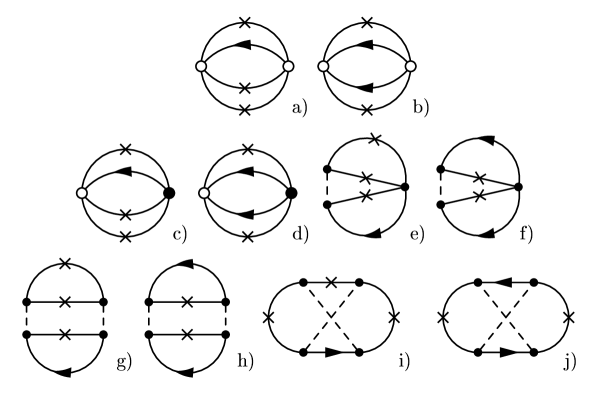
Figure 2: Subleading contribution of chiral order $Q^{7}$.

In Fig. 2 we collected all diagrams of chiral order $Q^{7}$. Here we introduced two types of 2-nucleon vertices. The filled circle represents the full vertex of (31) proportional to $g_{0,1}+g_{A}^{2}/4$ and the open circle the counter term proportional to $g_{A}^{2}/4$. The dashed line is the pion propagator and the directed solid line the free space nucleon propagator. We point out that the diagrams b), d), f), h) and j) in Fig. 2 are divergent. The leading chiral contribution of the sum of all diagrams, however, is finite after including the appropriate counter term in the spin triplet channel.

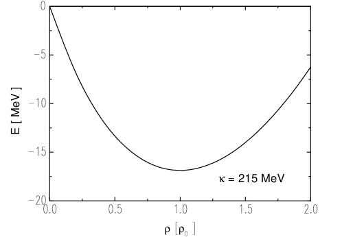
Figure 3: The equation of state for isospin symmetric nuclear matter.

It is instructive also to display the non relativistic form of the Lagrangian density (31) as suggested by Weinberg [1] in the context of the nucleon-nucleon scattering problem

$${\mathcal{L}}_{int}(k_{F}) = \frac{g_{A}}{2\,f_{\pi}}\,\bar{N}\left(\vec{\sigma}\cdot\vec{\nabla}\right)\Big{(}{\vec{\pi}}\cdot{\vec{\tau}}\Big{)}\,N$$ (33)

$$+ \frac{1}{8\,f_{\pi}^{2}}\,\left(g_{0}(k_{F})+\frac{1}{4}\,g_{A}^{2}\right)\left(\bar{N}\,\vec{\sigma}\,\sigma_{2}\,\tau_{2}\,\bar{N}^{t}\right)\left(N^{t}\,\tau_{2}\,\sigma_{2}\,\vec{\sigma}\,N\right)$$

$$+ \frac{1}{8\,f_{\pi}^{2}}\,\left(g_{1}(k_{F})+\frac{1}{4}\,g_{A}^{2}\right)\left(\bar{N}\,\sigma_{2}\,\,\vec{\tau}\,\tau_{2}\,\bar{N}^{t}\right)\left(N^{t}\,\tau_{2}\,\vec{\tau}\,\sigma_{2}\,N\right)$$

with $N$ now a two component spinor field and $\bar{N}=N^{\dagger}$ for notational convenience. According to Weinberg the two-particle reducible diagrams are to be evaluated with static pions.

We therefore evaluate all diagrams of Fig. 2 with the appropriate non relativistic interaction vertices and static pion propagators. The solid line with a ’cross’ now represents the non relativistic limit of (32) and the directed solid line the free non relativistic nucleon propagator. For technical details we refer to [23]. Both schemes indeed lead to identical results for all diagrams.

In Fig. 3 our result for the isospin symmetric nuclear equation of state is shown. The relevant coupling $g_{0}+g_{1}$ is adjusted to obtain nuclear saturation at $k_{F,0}=265$ MeV. We emphasize that the coupling functions $g_{0,1}(k_{F})$ are to be determined from the nuclear equation of state. However there is a strong consistency constraint: according to our scale argument (30) the density dependence of the couplings $g_{0,1}(k_{F})$ must be weak for $k_{F}$ larger than typical small scales integrated out. If the nuclear saturation required a strong density dependence our scheme had to be rejected. The density independent set of parameters $g_{0}+g_{1}\simeq 3.2$, $g_{A}\simeq 1.26$, $m_{\pi}\simeq 140$ MeV and $f_{\pi}\simeq 93$ MeV give an excellent result for the equation of state. The empirical saturation density $k_{F,0}\simeq 265$ MeV and the empirical binding energy of 16 MeV are reproduced. The incompressibility with $\kappa\simeq 215$ MeV is also compatible with the empirical value $(210\pm 30)$ MeV of [24].

4 The chiral order parameter $\langle\bar{q}q\rangle$

The quark condensate, $\langle\bar{q}q\rangle(\rho)$, is an object of utmost interest. It measures the degree of chiral symmetry restoration in nuclear matter. Furthermore it is an important input for QCD sum rules [25] or the Brown-Rho scaling hypothesis [26]. According to the Feynman-Hellman theorem the quark condensate can be extracted unambiguously from the total energy, $E(\rho)$, of nuclear matter once the current quark mass dependence of $E(\rho,m_{Q})$ is known

$$\langle\bar{q}q\rangle(\rho) = \frac{1}{V}\,\frac{\partial}{\partial\,m_{Q}}\,E(\rho,m_{Q})$$ (34)

with $m_{Q}=m_{u}=m_{d}$. Recall that $E(\rho)/V=(m_{N}+\bar{E}(\rho))\,\rho$ is determined by the nuclear equation of state $\bar{E}(\rho)$. Since our chiral approach was set up to treat the pion dynamics and therewith the current quark mass dependence of the equation of state properly it is very much tailored to be applied to the quark condensate.

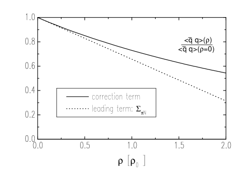
Figure 4: The quark condensate in isospin symmetric nuclear matter.

It is convenient to consider the relative change of the quark condensate since it is renormalization group invariant:

$$\frac{\langle\bar{q}\,q\rangle(\rho)}{\langle\bar{q}\,q\rangle(0)}=1-\frac{\Sigma_{\pi N}\,\rho}{m_{\pi}^{2}\,f_{\pi}^{2}}-\frac{\alpha_{\pi}(\rho)\,\rho}{2\,m_{\pi}\,f_{\pi}^{2}}\;.$$ (35)

The second term in (35) follows from the nucleon rest mass contribution to the total energy of nuclear matter together with the definition of the pion nucleon sigma term, $\Sigma_{\pi N}$:

$$\Sigma_{\pi N}=m_{Q}\,\langle N|\bar{q}\,q|N\rangle=m_{Q}\,\frac{d\,m_{N}}{d\,m_{Q}}\;.$$ (36)

The last term in (35) measures the sensitivity of the nuclear equation of state, $\bar{E}(\rho,m_{\pi})$, on the pion mass

$$\alpha_{\pi}(\rho) = -\frac{2\,m_{\pi}\,f_{\pi}^{2}}{\langle\bar{q}\,q\rangle(0)}\,\frac{\partial}{\partial\,m_{Q}}\,\bar{E}(\rho,m_{\pi})=\left(1+{\mathcal{O}}\left(m_{\pi}^{2}\right)\right)\frac{\partial}{\partial\,m_{\pi}}\,\bar{E}(\rho,m_{\pi})$$ (37)

where we consider now the current quark mass $m_{Q}=m_{Q}(m_{\pi})$ as a function of the physical pion mass. We emphasize that the second term in (35) written down first in [27, 28, 29] does not probe the nuclear many body problem and therefore should be considered with great caution. It is far from obvious that this term is the most important one at nuclear saturation density. The only term susceptible to nuclear dynamics is the last term in (35).

In Fig. 4 we present our result for the quark condensate in nuclear matter. We confront the ’leading’ term driven by $\Sigma_{\pi N}\simeq 45$ MeV with our result. The inclusion of pionic many body effects leads to a significantly less reduced quark condensate in nuclear matter. Note that here we do not include an explicit $m_{\pi}$ dependence of the coupling $g_{0,1}(k_{F})$ simply because there is not yet any reliable estimate available. Our results confirm calculations performed within the Brueckner [30] and Dirac-Brueckner [31] approach qualitatively insofar that the nuclear many body system appears to react against chiral symmetry restoration. They have strong implications for the QCD sum rule approach of hadron properties in nuclear matter.

References

References

- [1] S. Weinberg, Phys. Lett. B 251(1990) 288; Nucl. Phys. B 363 (1991) 3.
- [2] C. Ordonez, L. Ray and U. van Kolck, Phys. Rev. Lett. 13 (1994) 1982.
- [3] M. Lutz, in: The standard Model at Low Energies, hep-ph/9606301.
- [4] M. Lutz, nucl-th/9906028.
- [5] D.B. Kaplan, M.J. Savage and M.B. Wise, Nucl. Phys. B 534 (1998) 329; T. Mehen and I. Stewart, nucl-th/9809095, nucl-th/9906010.
- [6] T.D. Cohen and J. M. Hansen, nucl-th/9808038V3.
- [7] K.-G. Fogel, Arkiv f. Fysik 42 (1952) 4.
- [8] A. Friman, Acta Acad. Aboensis Math. et Phys. 41 (1957) 21.
- [9] J.V. Steele and R.J. Furnstahl, Nucl. Phys. A 645 (1999) 439.
- [10] M. Lutz, Nucl. Phys. A 642 (1998) 171c.
- [11] S. Weinberg, Phys. Rev. 166 1568 (1968); Physica 96 A (1979) 327.
- [12] A. Krause, Helv. Phys. Acta 63 (1990) 3.
- [13] J. Gasser, M.E. Sainio and A. Svarc, Nucl. Phys. B 307(1988) 779.
- [14] E. Jenkins and A.V. Manohar, Phys. Lett. B 255 (1991) 558.
- [15] V. Bernard, N. Kaiser and U.G. Meißner, Int. Jour. of Mod. Phys. E 4 (1995) 193; T.-S. Park, D.-P. Min and M. Rho, Phys. Rep. 233 (1993) 341.
- [16] P.J. Ellis and H-B. Tang, Phys. Rev. C 57 (1998) 3356.
- [17] S.R. Beane, D.R. Phillips and T.D. Cohen, Nucl. Phys. A 632 (1998) 445.
- [18] M. Mojzis, Eur. Phys. J C 2 (1998) 181.
- [19] R.E. Cutkosky, J. Math. Phys. 1 (1960) 429.
- [20] T. Mehen and I. Stewart, nucl-th/9901064.
- [21] M. Lutz, in preparation.
- [22] M. Beiner et al, Nucl. Phys. A 238 (1975) 29.
- [23] M. Lutz, B. Friman and Ch. Appel, in preparation.
- [24] J.P. Blaizot, Phys. Rep. 64 (1980) 172.
- [25] T. Hatsuda and Su H. Lee, Phys. Rev. C 46 (1992) R 34.
- [26] G.E. Brown and M. Rho, Phys. Rev. Lett. 66 (1991) 2720.
- [27] E.G. Drukarev and E.M. Levin, Nucl. Phys. A 511 (1990) 679.
- [28] M. Lutz, S. Klimt and W. Weise, Nucl. Phys. A 542 (1992) 521.
- [29] T.D. Cohen, R.J. Furnstahl and D.K. Griegel, Phys. Rev. C 45 (1992) 1881.
- [30] G.Q. Li and C.M. Ko, Phys. Lett. B 338 (1994) 118.
- [31] R. Brockmann and W. Weise, Phys. Lett. B 367 (1996) 40.