SU(3) quasi-dynamical symmetry as an organizational mechanism for generating nuclear rotational motions

Abstract

The phenomenological symplectic model with a Davidson potential is used to construct rotational states for a rare-earth nucleus with microscopic wave functions. The energy levels and $E2$ transitions obtained are in remarkably close agreement (to within a few percent) with those of the rotor model with vibrational shape fluctations that are adiabaticallly decoupled from the rotational degrees of freedom. An analysis of the states in terms of their SU(3) content shows that SU(3) is a very poor dynamical symmetry but an excellent quasi-dynamical symmetry for the model. It is argued that such quasi-dynamical symmetry can be expected for any Hamiltonian that reproduces the observed low-energy properties of a well-deformed nucleus, whenever the latter are well-described by the nuclear rotor model.

I Introduction

A microscopic theory of nuclear structure would be very incomplete without a satisfactory description of nuclear rotational states in terms of many-nucleon quantum mechanics. However, while the states of a truly rigid rotor can be handled with ease [1], they do not have square-integrable wave functions in either a spherical vibrational-model or many-nucleon Hilbert space. Moreover, the expansion of liquid-like, soft-rotor, wave functions on any spherical basis is slowly convergent. This means that many major shells are required for a realistic shell-model theory of nuclear rotational states. It also means that a realistic calculation of nuclear rotational states in terms of interacting nucleons, without a priori knowledge of the kinds of correlations to expect, is an impossibly difficult task. The fact remains that nuclear rotational bands are exceedingly simple; they are essentially characterized by a few intrinsic quadrupole moments and moments of inertia. Furthermore, they are observed in a wide range of nuclei throughout the periodic table. Thus, it would appear that the phenomenon is remarkably robust and relies very little, for its existence, on the details of the two-nucleon interaction.

As demonstrated by calculations within the framework of the nuclear symplectic model [2, 3, 4], it is possible to construct model rotational states with many-nucleon wave functions. The problem is to understand why the model works as well as it does; i.e, why the many residual interactions that strongly break symplectic symmetry, by mixing states of different irreps, do not destroy the predictions of the model.

To understand this, the effects of the dominant symmetry breaking interactions have been explored one at a time. It has been shown that, while a spin-orbit interaction may mix SU(3) irreps strongly, it does so, in large-dimensional irreps, in a highly coherent way such that the rotational spectrum of the model survives [5]. Similar coherent mixings of SU(3) irreps by pairing forces were found while investigating the transition of a many-fermion model [6] from a superconducting phase to a rotational phase with variation of the relative strengths of short-range (pairing) and long-range (quadrupole-quadrupole) interactions [7]. In this paper we examine in some detail the very strong mixing of major harmonic-oscillator shells and SU(3) irreps, within the framework of the symplectic model. Again the mixings are extraordinarily coherent. We refer to this coherent mixing as a quasi-dynamical symmetry [7, 8].

We conjecture that, because the residual interactions separately preserve quasi-dynamical symmetry, they continue to do so when combined for suitable ranges of their strengths. This conjecture is strongly supported by the observation of rotational states in nuclei which demonstrates unequivocally that they do survive.

The discovery of quasi-dynmical symmetry gives optimism that realistic calculations of rotational states, which simultaneously take into account the mixings between major shells and, for example, the effects of spin-orbit and short-range (e.g., pairing) interactions, may be possible. Up to the present time such calculation have not been possible except within the framework of a highly constrained (e.g., Hartree-Bogolyubov) approximation.

The calculations reported here are carried out with a simple Davidson interaction potential [9]. This interaction preserves a higher, symplectic model, symmetry which makes calculations in a very large multi-shell space possible. With this interaction, the Hamiltonian for a diatomic molecule was recently diagonalized by a simple non-linear transformation from a spherical vibrator basis to a soft rotor basis using an $\mbox{\lfrak su}(1,1)$ spectrum generating algebra (isomorphic to $\mbox{\lfrak sp}(1,{\mathbb{R}})$) [10]. A similar transformation [11, 10] gives rotational states in the Bohr-Mottelson collective model [12].

For a many-nucleon nucleus, one can construct a Hamiltonian comprising the many-nucleon kinetic energy, a spherical shell model potential, and the same Davidson potential as used to obtain rotational states in the pheomenological Bohr-Mottelson model. The Davidson potential is a scalar function of the nuclear quadrupole moments expressed in terms of nucleon coordinates. Thus, it is microscopic and rotationally-invariant. More importantly, it is expressible in terms of an $\mbox{\lfrak sp}(3,{\mathbb{R}})$ spectrum generating algebra and and gives a Hamiltonian that is diagonalizable within a single irrep of the symplectic model [2, 3, 4]. We are not able to give analytical expressions for its wave functions, as we were [10] for the diatomic molecule and Bohr-Mottelson model. But, we are able to compute its states numerically and expand them on a spherical shell-model basis. This is done by diagonalizing the Hamiltonian in a basis that reduces the dynamical subalgebra chain

$$\mbox{\lfrak sp}(3,{\mathbb{R}})\supset\mbox{\lfrak su}(3)\supset\mbox{\lfrak so}(3)\,,$$ (1)

where $\mbox{\lfrak su}(3)$ is the symmetry algebra of the spherical harmonic oscillator shell model [13].

Symplectic model calculations in an $\mbox{\lfrak su}(3)\supset\mbox{\lfrak so}(3)$ basis have been developed to a fine art using VCS (vector coherent state) methods [14, 15] to calculate matrix elements. Furthermore, they can be carried out in large spaces with relative ease.

An important property of the $\mbox{\lfrak sp}(3,{\mathbb{R}})$ algebra is that it contains, as a subalgebra, a spectrum generating algebra for a rigid-rotor model, namely Ui’s $[{\mathbb{R}}^{5}]\mbox{\lfrak so}(3)$ algebra [16]. However, one cannot diagonalize a symplectic model Hamiltonian in a basis that reduces the subalgebra chain

$$\mbox{\lfrak sp}(3,{\mathbb{R}})\supset[{\mathbb{R}}^{5}]\mbox{\lfrak so}(3)\supset\mbox{\lfrak so}(3)\,,$$ (2)

because, as mentioned above, rigid-rotor wave functions are not expandable in a shell-model basis (in technical terms, the decomposition is not a direct sum; it is a direct integral.). One notes, however, that the Hamiltonian we are considering as a model of a soft rotor has two components: a spherical shell model part which reduces the $\mbox{\lfrak sp}(3,{\mathbb{R}})\supset\mbox{\lfrak su}(3)\supset\mbox{\lfrak so}(3)$ chain and a Davidson potential which reduces $\mbox{\lfrak sp}(3,{\mathbb{R}})\supset[{\mathbb{R}}^{5}]\mbox{\lfrak so}(3)\supset\mbox{\lfrak so}(3)$. Thus, we expect results that lie between the two limits. In fact, the results of our calculations prove to be such that both $[{\mathbb{R}}^{5}]\mbox{\lfrak so}(3)$ and $\mbox{\lfrak su}(3)$ are extremely good quasi-dynamical symmetries. This is a remarkable result, because although $\mbox{\lfrak su}(3)$ and the rigid-rotor algebra have similar algebraic structures, they have very different physical interpretations.

A Lie algebra g is said to be a quasi-dynamical symmetry for a Hamiltonian $H$ if the matrix elements of g between a set of eigenstates of $H$ are equal to those of an irrep of g, even though the eigenstates in question do not belong to a subspace of the Hilbert space for $H$ that is irreducible under the action of g. At first sight this would be appear to be an unlikely physical situation. Indeed, if matrix elements of an algebra g were found in some situation to be equal to those of an irrep, one might be tempted to infer that g is a full dynamical symmetry for the Hamiltonian. The soft rotor model is the prototype of a situation where this is not the case, as we now show.

Let $\{\Phi_{KLM}(\beta,\gamma)\}$ denote a basis of wave functions for a rigid rotor with intrinsic quadrupole moments

$$\bar{Q}_{0}=k\beta\cos\gamma\,,\quad\bar{Q}_{1}=\bar{Q}_{-1}=0\,,\quad\bar{Q}_{2}=\bar{Q}_{-2}={1\over\sqrt{2}}k\beta\sin\gamma\,,$$ (3)

where $k$ is a suitable constant, cf. Eq. (25). Then soft-rotor wave functions can be expressed

$$\Psi_{\alpha KLM}=\int f_{\alpha}(\beta,\gamma)\,\Phi_{KLM}(\beta,\gamma)\,{\rm d}v\,,$$ (4)

where d$v$ is a suitable volume element for $\beta$ and $\gamma$. One finds that the matrix elements between all states of the same $\alpha$ are equal to those of a rigid rotor of deformation

$$\langle\bar{Q}_{0}\rangle=\int k\beta\cos\gamma\,f_{\alpha}(\beta,\gamma)\,{\rm d}v\,,\quad\langle\bar{Q}_{2}\rangle=\int{1\over\sqrt{2}}k\beta\sin\gamma\,f_{\alpha}(\beta,\gamma)\,{\rm d}v\,.$$ (5)

Thus, the states of a given $\alpha$ span an embedded representation of the rigid-rotor algebra in the terminology of ref. [17] and we say that the rigid-rotor algebra is a quasi-dynamical symmetry for the soft rotor.

An examination of the physics of the situation quickly reveals that the rigid-rotor algebra is a quasi-dynamical symmetry whenever the rotations are adiabatic relative to the complementary vibrational motions. Thus, one obtains the rigid-rotor algebra as a quasi-dynamical symmetry for a rotor-vibrator Hamiltonian whenever the rotational-vibrational (i.e., Coriolis and centrifugal) coupling interactions are negligible or omitted. They can be taken into account subsequently, as quasi-dynamical symmetry-breaking perturbations, as is standard in the pheomenological rotor model.

Now it is known [18] that the $\mbox{\lfrak su}(3)$ algebra contracts to the rigid-rotor algebra $[{\mathbb{R}}^{5}]\mbox{\lfrak so}(3)$ and that this contraction is realized for large-dimensional irreps of $\mbox{\lfrak su}(3)$. Thus, we say that $\mbox{\lfrak su}(3)$ is a quasi-dynamical symmetry for a sequence of states if their expansions on an $\mbox{\lfrak su}(3)$ basis are of the form

$$\Psi_{\alpha KLM}=\sum_{\lambda\mu}C_{\alpha\lambda\mu}\Phi^{\lambda\mu}_{KLM}\,,$$ (6)

where $\{\Phi^{\lambda\mu}_{KLM}\}$ is a basis of states of a large-dimensional $\mbox{\lfrak su}(3)$ irrep of highest weight $(\lambda,\mu)$. Note that shell-model states can always be expanded on an $\mbox{\lfrak su}(3)$ basis. However, we only obtain $\mbox{\lfrak su}(3)$ as a quasi-dynamical symmetry if the coefficients $\{C_{\alpha\lambda\mu}\}$ are independent of $KLM$ for a useful range of values of the latter.

The fact that $\mbox{\lfrak su}(3)$ is a good quasi-dynamical symmetry for major-shell mixing Hamiltonians is extremely important for achieving the eventual goal of including $\mbox{\lfrak sp}(3,{\mathbb{R}})$ symmetry-breaking interactions in the symplectic model. For although, interactions like the spin-orbit and pairing interactions break $\mbox{\lfrak sp}(3,{\mathbb{R}})$, they have been shown to preserve quasi-dynamical $\mbox{\lfrak su}(3)$ symmetry [5, 7]. This is expected to occur, to a good approximation, whenever the rotational motions one is describing are known from experiment to be adiabatic.

The concept of quasi-dynamical symmetry can be regarded simply as a group-theoretical expression of the standard methods for handling adiabatic decoupling of collective motions along the lines of the Born-Oppenheimer approximation [20] and the standard nuclear rotor model. A formulation in the precise language of group theory has the advantage that it opens the concept up to more general application. An overview of the concept was given in a recent conference report [8].

In Sect. II, the Hamiltonian of the nuclear symplectic model is described and the physical motivation behind the model in connection with Bohr-Mottelson collective model [12] is explained. Sect. III defines the $\mbox{\lfrak sp}(3,{\mathbb{R}})$ and its subalgebras relevant to this analysis. Sect. IV describes the construction of basis states and matrix elements within the three dimensional harmonic oscillator space. The results are given in Sect. V and some conclusions are drawn in Sect. VI

II The Symplectic Model Hamiltonian

The Hamiltonian of the nuclear symplectic model, in its simplest form, consists of two parts:

$$H=H_{0}+V(Q)\,;$$ (7)

a three dimensional many-particle harmonic oscillator (shell-model) Hamiltonian

$$H_{0}=\sum_{n=1}^{A}\left({\frac{p_{n}^{2}}{2m}}+{\frac{1}{2}}m\omega^{2}x_{n}^{2}\right)$$ (8)

and a collective potential $V(Q)$, where $Q$ is the quadrupole tensor for the nucleus.

The collective potential $V(Q)$ is a rotationally-invariant function of the quadrupole moments. In a Cartesian basis, the quadrupole moments for a nucleus are given by

$$Q_{ij}={\mathbb{Q}}_{ij}-\textstyle\frac{1}{3}\delta_{ij}\sum_{k=1}^{3}{\mathbb{Q}}_{kk}\,,$$ (9)

where ${\mathbb{Q}}$ is a monopole-quadrupole tensor with components

$${\mathbb{Q}}_{ij} = \sum_{n=1}^{A}(x_{ni}-X_{i})(x_{nj}-X_{j})$$ (10)

$$= \sum_{n=1}^{A}x_{ni}x_{nj}-\frac{1}{A}\sum_{m,n=1}^{A}x_{mi}x_{nj}\,,$$ (11)

and $\{X_{i}\}$ are the components of the center-of-mass vector ${\bf X}={1\over A}\sum_{n}{\bf x}_{n}$. Removal of the center-of-mass contribution to the quadrupole moments in this way, ensures that the spurious $N$-phonon center-of-mass states of the Hamiltonian remain, unmixed with other states, at an excitation energy of $N\hbar\omega$.

A general, rotationally-invariant potential can be expressed

$$V(Q)=V(Q\cdot Q,Q\cdot Q\times Q)\,,$$ (12)

as a function of the quadratic and cubic scalars

$$Q\cdot Q = \sum_{\mu=-2}^{2}(-1)^{\mu}Q_{-\mu}Q_{\mu}\;\propto{\rm Tr}Q^{2}\,,$$ (13)

$$Q\cdot Q\times Q = \sum_{\mu,\nu,\rho=-2}^{2}(-1)^{\mu}(2\nu;2\rho|2\mu)Q_{-\mu}Q_{\nu}Q_{\rho}\;\propto{\rm Tr}Q^{3}\,,$$ (14)

where

$\displaystyle Q_{\mu}=\sum\nolimits_{n}r_{n}^{2}Y_{2\mu}(\hat{\bf{r}}_{n})$

with $r_{n}=\left|{\bf x}_{n}-{\bf X}\right|$ and $\hat{\bf{r}}_{n}=({\bf x}_{n}-{\bf X})/r_{n}$. In the study reported in this article, the collective potential is taken to be the Davidson potential

$$V(Q)=\chi\left(Q\cdot Q+\frac{\varepsilon}{Q\cdot Q}\right)\,.$$ (15)

This potential is shown as a function of $\bar{Q}_{0}=\sqrt{Q\cdot Q}$ in Fig. 1.

The value of the parameter $\varepsilon$ determines the value of $\bar{Q}_{0}$ at which the potential has its minimum value. Thus, $\varepsilon$ is chosen such the potential has a minimum at the observed deformation of the nucleus under investigation. The strength $\chi$ of the potential is then set such that the lowest energy $(L=0)$ wave function that emerges is such that the expectation value ${\langle Q\cdot Q\rangle}$ in this state is equal to the value of $\bar{Q}_{0}^{2}$ at which the potential is a minimum. We refer to this as the self-consistent value of $\chi$.

III The symplectic algebra and its subalgebras

The quadrupole moments $\{Q_{\mu}\}$, the many-nucleon kinetic energy $\sum_{n}p_{n}^{2}/2m$, and the harmonic oscillator potentional ${\frac{1}{2}}m\omega^{2}\sum_{n}r_{n}^{2}$ are all elements of an $\mbox{\lfrak sp}(3,{\mathbb{R}})$ Lie algebra. Thus, $\mbox{\lfrak sp}(3,{\mathbb{R}})$ is a spectrum generating algebra for $H$; i.e., it is the Lie algebra of a dynamical group for $H$. It folows that the eigenstates of $H$ belong to a single irreducible representation of Sp$(3,{\mathbb{R}})$.

The complex extension $\mbox{\lfrak sp}_{{\mathbb{C}}}(3,{\mathbb{R}})$ of $\mbox{\lfrak sp}(3,{\mathbb{R}})$ is spanned by the operators (in a Cartesian coordinate system)

$$A_{ij} = \sum_{n=1}^{A}b_{ni}^{\dagger}b_{nj}^{\dagger}-\frac{1}{A}\sum_{m,n=1}^{A}b_{mi}^{\dagger}b_{nj}^{\dagger}\,,$$ (16)

$$B_{ij} = \sum_{n=1}^{A}b_{ni}b_{nj}-\frac{1}{A}\sum_{m,n=1}^{A}b_{mi}b_{nj}\,,$$ (17)

$$C_{ij} = \frac{1}{2}\sum_{n=1}^{A}(b_{ni}^{\dagger}b_{nj}+b_{nj}b_{ni}^{\dagger})-\frac{1}{2A}\sum_{m,n=1}^{A}(b_{mi}^{\dagger}b_{nj}+b_{nj}b_{mi}^{\dagger})\,,$$ (18)

where $b^{\dagger}_{ni}$ and $b_{ni}$ are the dimensionless harmonic oscillator raising and lowering (boson) operators

$$b_{ni}^{\dagger} = \frac{1}{b_{0}\sqrt{2}}\left(x_{ni}-\frac{i}{m\omega}p_{ni}\right)\,,$$

$$b_{ni} = \frac{1}{b_{0}\sqrt{2}}\left(x_{ni}+\frac{i}{m\omega}p_{ni}\right)\,,$$

in units of the oscillator length $b_{0}=(\hbar/m\omega)^{1/2}$. The latter operators satisfy the commutation relations

$${[b_{mi},b_{nj}^{\dagger}]} = \delta_{mn}\delta_{ij}{\mathbb{I}}\,,$$ (19)

$${[b_{ni},{\mathbb{I}}]} = {[b_{ni}^{\dagger},{\mathbb{I}}]}=0\,,$$ (20)

$${[b_{mi},b_{nj}]} = {[b_{mi}^{\dagger},b_{nj}^{\dagger}]}=0\,,$$ (21)

of a Heisenberg-Weyl algebra.

The symplectic algebra $\mbox{\lfrak sp}(3,{\mathbb{R}})$ contains many subalgebras, including the $\mbox{\lfrak u}(3)\supset\mbox{\lfrak su}(3)$ chain of Elliott’s SU(3) model [13] and the $\mbox{\lfrak rot}(3)$ $(=[{\mathbb{R}}^{5}]\mbox{\lfrak so}(3))$ rigid-rotor algebra of Ui’s model [16]. The $\mbox{\lfrak u}(3)$ subalgebra is spanned by the $\{C_{ij}\}$ operators. One sees, for example, that $\mbox{\lfrak u}(3)$ contains the harmonic oscillator Hamiltonian $H_{0}=\hbar\omega\sum_{i=1}^{3}C_{ii}$ as an element. The $\mbox{\lfrak rot}(3)$ algebra is spanned by three angular momentum operators

$\displaystyle L_{i}=-i(C_{jk}-C_{kj})\,,\quad(i,j,k\;{\rm cyclic})\,,$

and five components $\{Q_{\mu};\mu=0,\pm 1,\pm 2\}$ of the $L=2$ quadrupole tensor $Q$.

The Cartesian components of the monopole-quadrupole tensor are expressed

$${\mathbb{Q}}_{ij}=b_{0}^{2}\left[A_{ij}+\textstyle\frac{1}{2}(C_{ij}+C_{ji})+B_{ij}\right]\,.$$ (22)

The spherical components of the quadrupole operators are

$$Q_{\mu}=b_{0}^{2}\sqrt{3}(A_{2\mu}+C_{2\mu}+B_{2\mu})\,.$$ (23)

One sees that the part of $Q_{\mu}$ that commutes with $H_{0}$ is the $\mbox{\lfrak su}(3)$ quadrupole operator

$\displaystyle{\cal Q}_{\mu}=b_{0}^{2}\sqrt{3}C_{2\mu}\,.$

Thus, $\mbox{\lfrak su}(3)$ can be viewed as the projection of the $\mbox{\lfrak rot}(3)$ algebra onto the space of operators that leave spherical harmonic oscillator shells invariant.

An irrep of $\mbox{\lfrak u}(3)$ is characterized by a highest weight state $|\phi\rangle$ and a corresponding highest weight $\omega=(\omega_{1},\omega_{2},\omega_{3})$ defined such that

$\displaystyle C_{ij}|\phi\rangle=0\text{ for }i<j\,,\quad C_{ii}|\phi\rangle=\omega_{i}|\phi\rangle\,.$

Such an irrep remains irreducible on restriction to its $\mbox{\lfrak u}(1)+\mbox{\lfrak su}(3)\subset\mbox{\lfrak u}(3)$ subalgebra and has $\mbox{\lfrak u}(1)+\mbox{\lfrak su}(3)$ highest weight $N(\lambda\mu)$, where

$\displaystyle N=\omega_{1}+\omega_{2}+\omega_{3}\,,\quad\lambda=\omega_{1}-\omega_{2}\,,\quad\mu=\omega_{2}-\omega_{3}\,.$

An irrep of the rigid-rotor algebra, is characterized by an intrinsic state which is an eigenstate of the quadrupole-moment operators with eigenvalues $\{\bar{Q}_{\mu}\}$ that are related to the shape variables of the Bohr-Mottelson collective model [12] by

$$\overline{Q}_{0} = \sqrt{\frac{9}{5\pi}}AR_{0}^{2}\beta\cos\gamma\,,$$ (24)

$$\overline{Q}_{\pm 2} = \sqrt{\frac{9}{10\pi}}AR_{0}^{2}\beta\sin\gamma\,,$$ (25)

$$\overline{Q}_{\pm 1} = 0\,,$$ (26)

where $A$ is the mass number, $R_{0}$ is a nuclear radius, and $\beta$ and $\gamma$ are deformation and asymmetry parameters, respectively.

It is useful to note that the elements of $\mbox{\lfrak sp}_{{\mathbb{C}}}(3,{\mathbb{R}})$ are all compnents of U(3) tensors, i.e., they transform according to irreducible representations of $\mbox{\lfrak u}(3)$; the operators $\{A_{ij}\}$ are components of an irreducible tensor $A$ of highest weight $\{200\}$, the $\{B_{ij}\}$ are components of an irrreducible tensor $B$ of highest weight $\{00-2\}$, the operators $\{C_{ij},C_{ji},C_{ii}-C_{jj};i\leq j\}$ are components of an irreducible $\mbox{\lfrak su}(3)$ tensor $C^{(11)}$ of $\mbox{\lfrak su}(3)$ highest weight $(11)$ ($\mbox{\lfrak u}(3)$ highest weight $\{10-1\}$), and $H_{0}=\hbar\omega\sum_{i=1}^{3}C_{ii}$ is a u(3) scalar; a tensor of highest weight $\{000\}$.

Now observe that the first term, $H_{0}$, of the Hamiltonian of Eq. (7) is SU(3) (and U(3)) invariant whereas the second term is invariant under the dynamical group ROT(3) $(=[{\mathbb{R}}^{5}]$SO(3)) of a rigid rotor. Thus, the two components, $H_{0}$ and $V(Q)$, of the Hamiltonian respectively reduce the two subalgebra chains:

$\displaystyle\begin{array}[]{ccc}&\mbox{\lfrak sp}(3,{\mathbb{R}})&\\ \quad\swarrow&&\searrow\\ \mbox{\lfrak su}(3)&&\quad\mbox{\lfrak rot}(3)\\ \quad\searrow&&\swarrow\\ &\mbox{\lfrak so}(3)&\end{array}$

This implies that the eigenstates of $H=H_{0}+V(Q)$ are intermediate between those of the SU(3) and rigid-rotor models. We show in the following that, in fact, both SU(3) and ROT(3) are remarkable good quasi-dynamical symmetries for this Hamiltonian.

IV Basis states and matrix elements

A unitary irrep of $\mbox{\lfrak sp}(3,{\mathbb{R}})$, within the shell-model space of a mass-$A$ nucleus, is characterized by a lowest-weight state $|\sigma\text{lw}\rangle$, with weight $\sigma=(\sigma_{1},\sigma_{2},\sigma_{3})$, defined by the equations

$$B_{ij}|\sigma\text{lw}\rangle=0\,,\quad C_{ij}|\sigma\text{lw}\rangle=0\text{ for }i<j,\quad C_{ii}|\sigma\text{lw}\rangle=\sigma_{i}|\sigma\text{lw}\rangle\,.$$ (27)

When $\sigma$ is a triple of positive integers or of positive half-odd integers, the corresponding irrep is either a discrete series representation or, for mass number $A<6$, a limit of a discrete series irrep.

Let $\{|\sigma\alpha\rangle\}$ denote an orthonormal basis for the subspace of states of an $\mbox{\lfrak sp}(3,{\mathbb{R}})$ irrep, of lowest weight $\sigma$, that satisfy the equation

$$B_{ij}|\sigma\alpha\rangle=0\,.$$ (28)

We refer to these states as vacuum states for the corresponding $\mbox{\lfrak sp}(3,{\mathbb{R}})$ irrep. They are a basis for a $\mbox{\lfrak u}(3)$ irrep of highest weight $\sigma$. Moreover, it is known that a basis for an $\mbox{\lfrak sp}(3,{\mathbb{R}})$ irrep can be constructed by acting on the vacuum states with polynomials in the $\{A_{ij}\}$ raising operators. Let

$$Z^{(n)}_{KLM}(A)=[A\times A\times\ldots\times A]^{(n)}_{KLM}$$ (29)

denote a product of $N$ symplectic raising operators coupled to the $(KLM)$ component of a U(3) tensor operator $Z^{(n)}(A)$ of highest weight $n=(n_{1},n_{2},n_{3})$, where $n_{1}$, $n_{2}$, and $n_{3}$ run over the even-integer values for which

$$n_{1}\geq n_{2}\geq n_{2}\geq 0\,,\quad n_{1}+n_{2}+n_{3}=2N\,.$$ (30)

Acting on the vacuum states with these tensor operators gives basis states

$$|\sigma n\rho\omega KLM\rangle=[Z^{(n)}(A)\times|\sigma\rangle]^{\rho\omega}_{KLM}$$ (31)

which reduce the subgroup chain

$$\matrix{{\rm Sp}(3,{\mathbb{R}})&\supset&{\rm U}(3)&\supset&{\rm SO(3)}&\supset&{\rm SO(2)}\cr\sigma&n\rho&\omega&K&L&&M\cr}.$$ (32)

These states are eigenstates of the harmonic oscillator hamiltonian

$$H_{0}|(\sigma n)\rho\omega KLM\rangle=(N_{0}+n_{1}+n_{2}+n_{3})\hbar\omega|(\sigma n)\rho\omega KLM\rangle\,,$$ (33)

where $N_{0}=\sigma_{1}+\sigma_{2}+\sigma_{3}$. However, although the basis states of Eq. (31) span the carrier space of an $\mbox{\lfrak sp}(3,{\mathbb{R}})$ irrep, they are not an orthonormal basis due to a multiplicity of U(3) subirreps labelled by the indices $n$ and $\rho$. Thus, it is necessary to take suitable linear combinations

$\displaystyle|\sigma\tau\omega KLM\rangle=\sum_{n\rho}(K^{\sigma}_{\omega})^{-1}_{n\rho,\tau}|\sigma n\rho\omega KLM\rangle$

to form an orthonormal basis. The K matrix coefficients are conveniently determined by vector coherent state (VCS) methods [14, 15]. The calculation of matrix elements of elements of the $\mbox{\lfrak sp}(3,{\mathbb{R}})$ Lie algebra in the corresponding orthonormal basis is also straightforward using VCS theory.

Matrix elements of the components $\{X_{klm}\}$ of an SU(3) tensor $X^{(pq)}$ are obtained from their $\mbox{\lfrak su}(3)$-reduced matrix elements using the generalized Wigner-Eckart theorem

$$\langle\sigma\nu^{\prime}\tau^{\prime}\omega^{\prime}K^{\prime}L^{\prime}M^{\prime}|X_{klm}|\sigma\tau\omega KLM\rangle = \sum_{\gamma}((\lambda\mu)KL;(pq)kl\|\gamma(\lambda^{\prime}\mu^{\prime})K^{\prime}L^{\prime})\,(LM;lm|L^{\prime}M^{\prime})$$ (35)

$$\times\langle\sigma\tau^{\prime}\omega^{\prime}\|X^{(pq)}\|\sigma\tau\omega\rangle_{\gamma}\,,$$

where $\lambda=\omega_{1}-\omega_{2}$, $\mu=\omega_{2}-\omega_{3}$, and $\gamma$ indexes the multiplicity of SU(3) irreps of highest weight $(\lambda^{\prime}\mu^{\prime})$ in the tensor product $(\lambda\mu)\times(pq)$; $(LM;lm|L^{\prime}M^{\prime})$ is an SO(3) Clebsch-Gordan coefficient and $((\lambda\mu)KL;(pq)kl\|\gamma(\lambda^{\prime}\mu^{\prime})K^{\prime}L^{\prime})$ is an SO(3)-reduced Clebsch-Gordan coefficient for SU(3).

SU(3)-reduced matrix elements of elements of the $\mbox{\lfrak sp}(3,{\mathbb{R}})$ Lie algebra are given, for example, in ref. [15]. To calculate matrix elements of $Q\cdot Q$, following Rosensteel [21], we start by normal ordering the expansion

$$Q\cdot Q = 3(A_{2}+C_{2}+B_{2})\cdot(A_{2}+C_{2}+B_{2})$$ (36)

$$= 6{\cal C}_{2}^{\mbox{\lfrak su}(3)}-3L^{2}+10H_{0}+10\sqrt{6}B_{0}+6A_{2}\cdot B_{2}+\{6C_{2}\cdot B_{2}+3B_{2}\cdot B_{2}+\text{h.c.}\}\,,$$ (37)

using the commutation relations

$$B_{2}\cdot A_{2}-A_{2}\cdot B_{2} = \textstyle\frac{10}{3}H_{0}\,,$$ (38)

$$B_{2}\cdot C_{2}-C_{2}\cdot B_{2} = \textstyle\frac{10}{3}\sqrt{6}B_{0}\,.$$ (39)

With such a normal-ordered expansion, i.e., with $B_{2}$ operators on the right and $A_{2}$ operators on the left, we do not have to include intermediate states external to the truncated space; consequently, the intermediate sums are minimized and the calculations are less time consuming. Optimization of the computations in this way is important because the number of basis states grows exponentially as the number of major oscillator shells in the calculation increases. For example, suppose we want to calculate matrix elements of $Q\cdot Q$ between states of a truncated space comprising the oscillator shells $N_{0}\hbar\omega$, $(N_{0}+2)\hbar\omega$, $(N_{0}+4)\hbar\omega$, $\ldots$, $(N_{0}+n)\hbar\omega$. Without normal ordering, we would have to include intermediate states in the calculation from the $(N_{0}+n+2)\hbar\omega$ shell. The number of extra states involved in the calculation would then be proportional to $n(n+1)$.

The first three terms in Eq. (37) are diagonal in the chosen basis with eigenvalues given by

$$\left\langle{\cal C}_{2}^{\mbox{\lfrak su}(3)}\right\rangle=\mathop{\textstyle\sum}\nolimits_{i}(\omega_{i}-\textstyle\frac{1}{3}N)(\omega_{i}-\textstyle\frac{1}{3}N-2i)=\textstyle\frac{2}{3}(\lambda^{2}+\mu^{2}+\lambda\mu+3\lambda+3\mu)\,,$$ (40)

$$\left\langle L^{2}\right\rangle=L(L+1)\,,\quad\quad\left\langle H_{0}\right\rangle=N\,.$$ (41)

The quadratic terms are expressible as $\mbox{\lfrak su}(3)$-coupled tensors using the identity

$$T_{2}^{(\lambda_{t}\mu_{t})}\cdot U_{2}^{(\lambda_{u}\mu_{u})}=\sqrt{5}\sum_{\rho(\lambda\mu)}\left\langle(\lambda_{t}\mu_{t})2;(\lambda_{u}\mu_{u})2\|(\lambda\mu)0\right\rangle_{\rho}\left[T^{(\lambda_{t}\mu_{t})}\times U^{(\lambda_{u}\mu_{u})}\right]^{\rho(\lambda\mu)}_{0}\,;$$ (42)

this gives

$$A_{2}\cdot B_{2} = \textstyle\frac{5}{6}\sqrt{6}(A\times B)^{(00)}+\textstyle\frac{1}{6}\sqrt{30}(A\times B)^{(22)}_{0}\,,$$ (43)

$$C_{2}\cdot B_{2} = \sqrt{5}(C\times B)^{(02)}_{0}\,,$$ (44)

$$B_{2}\cdot B_{2} = \textstyle\frac{2}{3}\sqrt{5}(B\times B)^{(04)}_{0}+\textstyle\frac{5}{3}(B\times B)^{(20)}_{0}\,.$$ (45)

The $\mbox{\lfrak su}(3)$-scalar component of $A_{2}\cdot B_{2}$ is related to the quadratic Casimir invariants of $\mbox{\lfrak sp}(3,{\mathbb{R}})$ and $\mbox{\lfrak su}(3)$

$\displaystyle(A\times B)^{(00)}=\textstyle\frac{1}{12}\sqrt{6}({\cal C}_{2}^{\mbox{\lfrak su}(3)}+\textstyle\frac{1}{3}H_{0}^{2}-4H_{0}-{\cal C}_{2}^{\mbox{\lfrak sp}(3,{\mathbb{R}})})\,,$

where

$$\left\langle{\cal C}_{2}^{\mbox{\lfrak sp}(3,{\mathbb{R}})}\right\rangle=\mathop{\textstyle\sum}\nolimits_{i}\sigma_{i}(\sigma_{i}-2i)=\textstyle\frac{2}{3}(\lambda_{0}^{2}+\lambda_{0}\mu_{0}+\mu_{0}^{2}+3\lambda_{0}+3\mu_{0})+\textstyle\frac{1}{3}N_{0}^{2}-4N_{0}\,,\\$$ (46)

with

$$\lambda_{0}=\sigma_{1}-\sigma_{2}\,,\quad\mu_{0}=\sigma_{2}-\sigma_{3}\,,\quad N_{0}=\sigma_{1}+\sigma_{2}+\sigma_{3}\,.$$ (47)

Combining the above results, Eq. (37) becomes

$$Q\cdot Q = -\textstyle\frac{5}{2}{\cal C}_{2}^{\mbox{\lfrak sp}(3,{\mathbb{R}})}+\textstyle\frac{17}{2}{\cal C}_{2}^{\mbox{\lfrak su}(3)}-3L^{2}+\textstyle\frac{5}{6}H_{0}+\sqrt{30}(A\times B)^{(22)}_{0}$$ (50)

$$+\{10\sqrt{6}B_{0}+6\sqrt{5}(C\times B)^{(02)}_{0}$$

$$+2\sqrt{5}(B\times B)^{(04)}_{0}+5(B\times B)^{(20)}_{0}+\text{h.c.}\}\,.$$

V Results

Calculations have been done for a typical heavy nucleus with oscillator energy $\hbar\omega=7.49$ MeV; a value appropriate for the ${}_{\;68}^{166}$Er nucleus. The deformation parameter $\varepsilon=1.01\times 10^{11}$ gives the minimum of the collective potential at $\beta_{{\rm in}}=0.35$; a value close to that inferred from the experimental $B(E2$:$2_{1}^{+}\rightarrow 0_{1}^{+})$ transition rate. We choose an $\mbox{\lfrak sp}(3,{\mathbb{R}})$ irrep with lowest weight $(327\frac{1}{2},249\frac{1}{2},249\frac{1}{2})$ (or equivalently, $826\frac{1}{2}(78,0)$ in a U(1) $\times$ SU(3) notation [3]). This irrep is deduced from an empirical formula for the intrinsic mass quadrupole moment of a deformed oscillator [22, 15]. The strength $\chi$ of the potential $V(Q)$ in Eq. (15) is varied in this study. The ratio between the potential and oscillator strengths determines the structure of the wave functions. Due to computational limitations, the space is restricted to states belonging to shells below $12\hbar\omega$; apart from this restriction there is no further truncation.

A Ground state band

Energy spectra for different $\chi$ values (in units of MeV) are given in Fig. 2. The results show ground state bands with rotational spectra and moments of inertia that decrease as $\chi$ increases. Moments of inertia, defined for each angular momentum state, by the expression

$${\cal J}_{L}=\frac{1}{2(E_{L}-E_{0})}L(L+1)$$ (51)

are shown in Table I.

TABLE I.: Moments of inertia for states of angular momentum $L$; the values in parenthesis are percentages relative to the value at $L=2$.

$L\;\backslash\;\chi$	1.67$\times$10-5 MeV	3.33$\times$10-5 MeV	1.67$\times$10-4 MeV	8.33$\times$10-4 MeV
2	207.62 MeV-1 (100.00%)	148.27 MeV-1 (100.00%)	70.10 MeV-1 (100.00%)	15.72 MeV-1 (100.00%)
4	207.44 (99.91%)	148.15 (99.92%)	70.04 (99.91%)	15.70 (99.89%)
6	207.16 (99.78%)	147.97 (99.80%)	69.94 (99.76%)	15.68 (99.72%)
8	206.78 (99.59%)	147.72 (99.63%)	69.79 (99.55%)	15.64 (99.49%)
10	206.29 (99.36%)	147.41 (99.42%)	69.61 (99.30%)	15.59 (99.20%)
12	205.71 (99.08%)	147.02 (99.16%)	69.40 (98.99%)	15.54 (98.85%)
14	205.02 (98.75%)	146.57 (98.86%)	69.14 (98.62%)	15.47 (98.43%)
16	204.22 (98.36%)	146.06 (98.51%)	68.84 (98.20%)	15.40 (97.95%)
18	203.33 (97.93%)	145.48 (98.12%)	68.50 (97.72%)	15.31 (97.41%)

The most remarkable result is that, for each of the interaction strengths shown, the spectra are almost identical to those of a rigid rotor with excitation energies very accurately proportional to $L(L+1)$. $B(E2)$ transition rates between adjacent states, shown for $\chi=3.33\times 10^{-4}$ MeV in Table II, are also in remarkably close agreement with those of a rigid rotor. These results are significant because, they give rotor model results with fully microscopic 166-particle wave functions. Thus, they provide us with the means to explore the rotational dynamics of a nucleus at the microscopic, many-nucleon, level. As a comparison, the results from Elliott’s SU(3) model are also given with the effective charge $e=2.04$. In the symplectic-Davidson model, $e=1$.

TABLE II.: The reduced quadrupole transition strength $B(E2:L\rightarrow L{-}2)$ in Weisskopf unit (W.u.) for the experimental data, SU(3) model, this model (with coupling constant $\chi=3.33\times 10^{-4}$ MeV), and a rigid rotor. Ratios of transition strengths to those of the the $2\to 0$ transition are given in parenthesis.

$L_{i}\rightarrow L_{f}$	experiment	SU(3)	Davidson	rigid rotor
$2\rightarrow 0$	$214\pm 10$ (1.00)	207 (1.00)	207 (1.00)	207 (1.00)
$4\rightarrow 2$	$311\pm 20$ (1.45)	295 (1.43)	295 (1.43)	296 (1.43)
$6\rightarrow 4$	$347\pm 45$ (1.62)	324 (1.57)	325 (1.57)	326 (1.57)
$8\rightarrow 6$	$365\pm 50$ (1.70)	338 (1.63)	339 (1.64)	340 (1.64)
$10\rightarrow 8$	$371\pm 46$ (1.73)	345 (1.68)	348 (1.68)	350 (1.69)
$12\rightarrow 10$	$376\pm 40$ (1.76)	349 (1.69)	353 (1.71)	356 (1.72)
$14\rightarrow 12$		350 (1.69)	356 (1.72)	361 (1.74)
$16\rightarrow 14$		350 (1.69)	357 (1.73)	365 (1.76)
$18\rightarrow 16$		349 (1.69)	358 (1.73)	367 (1.77)

A question of considerable interest is the nature of nuclear rotational energies. In the Bohr-Mottelson rotor model [12] rotational energies are interpreted as arising from the kinetic energy whereas in Elliott’s SU(3) model [13] they come from the potential energy. Since the symplectic model contains both a rigid-rotor and Elliott’s SU(3) models as limiting submodels, it is of considerable interest to see how it interpolates between the two limits. In the symplectic model, the kinetic energy operator is written

$$T=\textstyle\frac{1}{2}\hbar\omega\left[H_{0}-\sqrt{\textstyle{\frac{3}{2}}}(A_{0}+B_{0})\right]\,.$$ (52)

The contribution of the kinetic to the total calculated excitation energy is shown as a percentage for each state of the ground state band in Table III).

TABLE III.: The kinetic energy as a percentage of the total excitation energy for different values of the coupling constant $\chi$. The values of $\beta_{0}$ show the average deformation of the ($L=0$) ground state according to Eq. (25).

$L\;\backslash\;\chi$	1.67$\times$10-5 MeV	3.33$\times$10-5 MeV	1.67$\times$10${}^{-4}MeV$	8.33$\times$10-4 MeV
2	-31.95%	-21.57%	26.43%	9.46%
4	-31.93	-21.56	26.44	9.46
6	-31.90	-21.53	26.46	9.45
8	-31.85	-21.49	26.48	9.44
10	-31.79	-21.44	26.52	9.43
12	-31.72	-21.37	26.55	9.41
14	-31.64	-21.30	26.60	9.39
16	-31.54	-21.22	26.65	9.37
18	-31.43	-21.12	26.71	9.35
$\beta_{0}$	0.247	0.275	0.345	0.351

It can be seen that, for the smaller values of $\chi$, the kinetic energy gives a negative contribution to excitation energies. Its contribution is positive for larger values of $\chi$, but remains much less than that of the potential energy. Note, however, that because of the truncation to shells of $12\hbar\omega$ and below, the results shown for $\chi=8.33\times 10^{-4}$ MeV are not fully converged and are unreliable. Even so, since we obtain rotational bands in close agreement with the rotor model for a wide range of potential strengths, it is hard to avoid the inference that nuclear rotational energies are most likely not 100% kinetic in origin. If this is correct, it has considerable conceptual implications for the interpretation of nuclear rotational dynamics. We may continue, for convenience, to describe the cofactor of the $L(L+1)$ rotational energy as the inverse of a “moment of inertia”, but one should recognize that, if the excitation energy is not kinetic, the concept is misleading.

Another result of this study is that the moments of inertia as well as the kinetic energy portions of the excitation energy change less than 5% over the range of angular-momentum values considered. This result can be interpreted as signifying that the states of a band have a common intrinsic structure that changes little with increasing angular momentum. This interpretation becomes much more compelling when one observes the behaviour of the coefficients of the wave functions in the expansion

$$|\psi_{KLM}\rangle=\displaystyle\sum_{(\lambda\mu)}|{(\lambda\mu)KLM}\rangle C_{(\lambda\mu)KL}\,,$$ (53)

of the states of the ground state band in a U(3) $\supset$ SU(3) $\supset$ SO(3) basis. The coefficients are plotted for different $\chi$ values in Fig.  3. The figure shows clearly, that for all values of $\chi$ considered, the coefficients are essentially independent of $L$ and negligible for $K\not=0$. Moreover, for the larger $\chi$, this is in spite of a huge mixing of SU(3) irreps from many major shells. It follows that, while SU(3) is far from being a good dynamical symmetry, it remains an extrordinarily good quasi-dynamical symmetry according to the definition given in the Introduction and Refs. [7, 17].

Observe also that the distribution of U(3) irreps is dominated by the so-called stretched irreps; the stretched irreps are those of the sequence

$\displaystyle N_{0}(\lambda_{0},0)\,,\quad N_{0}+2(\lambda_{0}+2,0)\,,\quad N_{0}+4(\lambda_{0}+4,0)\,,\quad\ldots,\quad N_{0}+2n(\lambda_{0}+2n,0)\,,\quad\ldots\,.$

The value of the coupling constant for which the $L=0$ ground state of the model Hamiltonian has a deformation $\beta_{0}=0.350$ equal to $\beta_{\rm in}$, the value for which the Davidson potential is a minimum, was found by repeated calculation to be given by $\chi=3.33\times 10^{-4}$ MeV. We call this the self-consistent coupling constant. The spectrum of the ground band for this $\chi$ is displayed in Fig. 4 in comparison with the observed spectrum of ¹⁶⁶Er and that of the rigid rotor. One sees that the results track the rigid rotor more closely than they do experiment. This may be an artifact of the Davidson potential which continues to rise unrealistically at large deformation and excessively inhibits centrifugal stretching. We also computed the reduced electromagnetic transition strengths

$$B(E2:L_{i}\rightarrow L_{f})={\frac{2L_{f}+1}{2L_{i}+1}}\left({\frac{5}{16\pi}}\right)\left({\frac{eZ}{A}}\right)^{2}|\langle f||Q||i\rangle|^{2}\,.$$ (54)

The ratios of transition strengths, shown in parenthesis in Table II and also depicted in Fig. 5, are in extremely close agreement both with experiment and the rigid-rotor model. Their magnitudes shown in Fig. 4 are also in good agreement with experiment.

B Giant resonance bands

In addition to the ground-state rotational band, the symplectic model gives many excited bands. However, for a single $N_{0}(\lambda_{0},0)$ irrep, as considered here, without spin-orbit, pairing and other irrep-mixing interactions, the simple symplectic model has no low-lying excited bands any more than the SU(3) model has excited bands for a $(\lambda_{0},0)$ irrep. The lowest-energy excited bands of the simple symplectic model are associated with the giant monopole (breathing mode) and giant quadrupole resonance degrees of freedom.

For small values of $\chi$, these occur in the model, with a Davidson potential, at around $2\hbar\omega$. They are shown for several values of $\chi$ in Fig. 2; results for the self-consistent value are given in Fig. 6.

Two results are worth noting. The first is that the energies of the giant-resonance bands rise with increasing values of $\chi$ and become unrealistically high at the value considered appropriate for the ground state band. This we believe to be a reflection of the fact that, although the Davidson potential has many useful features, it rises too steeply away from the equilibrium deformation. The second notable result is that the symplectic model gives three monopole-quadrupole giant resonance bands; two of these, the $K=0$ and $K=2$ bands, occur also (albeit at much lower energy) in the Bohr-Mottelson model where they are associated with beta- and gamma-vibrations, respectively. However, whereas there is no $K=1$ one-phonon band in the Bohr-Mottelson model, such a band is non-spurious in the symplectic model which includes intrinsic vorticity degrees of freedom.

The monopole and quadrupole giant resonance states in real nuclei are believed to lie at energies close to $2\hbar\omega$. However, their strength is invariably fragmented and much of it lies in the continuum. Thus, we make no attempt to compare our results for the GR states with experiment. However, it is of interest to examine the structure of the wave functions. Fig. 7 shows the decomposition of the $K=0$ (giant-beta band) states in terms of their SU(3) components, for the self-consistent value of $\chi$, in comparison with the corresponding decomposition of the ground-band states. It can be seen that the amplitude coefficients (including their signs) are independent of angular momentum to a high degree of accuracy. It can also be seen that the coefficients for the two sets of states have the same signs except for those of the stretched states, which are of opposite sign. Note that the relative signs of the amplitude coefficients for different SU(3) subirreps are determined by SU(3) Clebsch-Gordan coeffients [24] and have no particular meaning, in general, except for the stretched states which all have the same sign. However, a change in the relative signs of coefficients between the ground and excited states is meaningful. Thus, it is fortuitous that the coefficients for the stretched states all have positive sign for the states of the ground state band because it highlights the fact that these coefficients change sign for the giant beta band. On reflection this is what one would expect for a giant-beta vibrational excitation (see Fig. 8).

VI Conclusion

The symplectic model is currently the only model that is capable of giving rotational states for heavy nuclei as eigenstates of a rotationally-invariant Hamiltonian in a realistic shell-model space. Thus, the ability of the model to give the energy levels and $E2$ transitions strengths between states for ground-state rotational bands, without the use of an effective charge, provides a powerful framework for understanding the dynamics of nuclear rotations in terms of interacting neutrons and protons.

Early applications of the model by Park et al. [4] were remarkably successful and raised many interesting questions. However, because of the severe truncations of the space that were necessary at the time, the reliability of the results could be questioned. In particular, one was concerned that the ability of the model to give correct moments of inertia might be lost on increasing the size of the model space. The results of the present calculations show that this is not the case.

A particularly interesting challenge was to learn how a model, without pair correlations, could give correct moments of inertia when it is known that the cranking model is only succesful when pairing correlations are included. The early calculations of Park et al. indicated that the dominant contribution to rotational energies came from the potential energy part of the Hamiltonian, thus calling into question the very concept of the moment of inertia as an inverse coefficient of the $L^{2}$ term in the kinetic energy. The results of the present calculation indicate that the inclusion of only stretched states, as in the calculation of Park et al., tends to exagerate this effect. Nevertheless, it confirms that the dominant component of the rotational energies comes from the potential energy; for the self-consistent value of $\chi$ only about 20% of the rotational energy comes from the kinetic energy in the present calculation.

In addition to investigating rotational states up to much higher angular momentum $(L=18)$, the present calculations have focussed on understanding the structure of rotational states in terms of their SU(3) content. We have shown that although there is huge mixing of SU(3) irreps from many major harmonic oscillator shells, the mixing is highly coherent and establishes SU(3) as a remarkably good quasi-dynamical symmetry for the model. Other calculations [17, 7], reviewed in [8], show that such quasi-dynamical symmetry is also conserved when SU(3) irreps are further mixed by spin-orbit and pairing forces. Thus, the results show that, as far as the calculation of $E2$ transition rates are concerned, the use of a single SU(3) irrep with an effective charge will give accurate results. However, for other observables, not related to elements in the SU(3) algebra, there is no reason whatever to expect effective charge methods to take account of the large mixing of SU(3) irreps observed.

The close agreement between the results of the symplectic model calculation and those of the rigid-rotor model, shows that, by definition, the rigid-rotor algebra is also an excellent quasi-dynamical symmetry for the symplectic model with a Davidson potential. But again, for observables not related to the rigid-rotor algebra, such as electron scattering current operators, one cannot predict what the results will be by purely algebraic methods.

The fact that two competing dynamical subgroup chains, although very different in their physical content, can both be good quasi-dynamical symmetries is remarkable but understandable. It can happen because, for large-dimensional representations and states of relatively low angular momentum, an SU(3) irrep contracts to an irrep of the rigid-rotor algebra [18]. Thus, it transpires that the lower angular-momentum states of a large-dimensional SU(3) irrep belong to an embedded representation [17] of the rigid-rotor algebra and vice-versa.

Having demonstrated that symplectic model calculations with phenomenological (albeit microscopically expressable) potentials have the ability to describe nuclear rotational states, our next goal would be ideally to perform calculations within the same (large) shell model space but with realistic two-nucleon interactions. Such calculations can and have been contemplated for light nuclei [19]. But they are computer intensive and impractical for heavy rotational nuclei. We would even like to go further and include spin-orbit and short-range (e.g., pairing) interactions which mix different $\mbox{\lfrak sp}(3,\mathbb{R})$ irreps. We would like to carry out calculations for superdeformed bands [26, 27] as well as for normally deformed low-lying rotational bands of heavy nuclei. Superdeformed bands are naturally associated with excited representations of the symplectic model which fall into the low-energy domain (as do Nilsson model states) as a consequence of shell effects in a deformed shell model. The challenge is to explain why they do not mix more readily with the large density of less deformed low-energy states. We believe that symplectic symmetry and su(3) quasi-dynamical symmetry has the potential to answer such questions.

It is unlikely that such calculations will ever be done in a shell-model space sufficiently large to ensure convergence of the results. However, the results of the present study and previous investigations of mixing SU(3) irreps with spin-orbit [17] and pairing interactions[7] imply that, when experiment finds states of a nucleus that are fitted well by the rotor model and to have a large deformation, then we have reason to believe that SU(3) is a good quasi-dynamical symmetry for these states. Armed with this information, one can hope to design realistic mixed SU(3) calculations within large spaces. In particular, one can calculate just one representative angular momentum state for each band, with the understanding that the coefficients should be the same (to a good approximation) for all other states of the band. Alternatively, one could carry out calculations in an intrinsic space which includes just the highest weight states for the contributing SU(3) irreps.

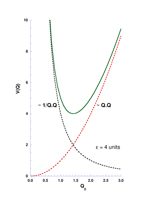
FIG. 1.: The Davidson potential; its two components are shown separately.

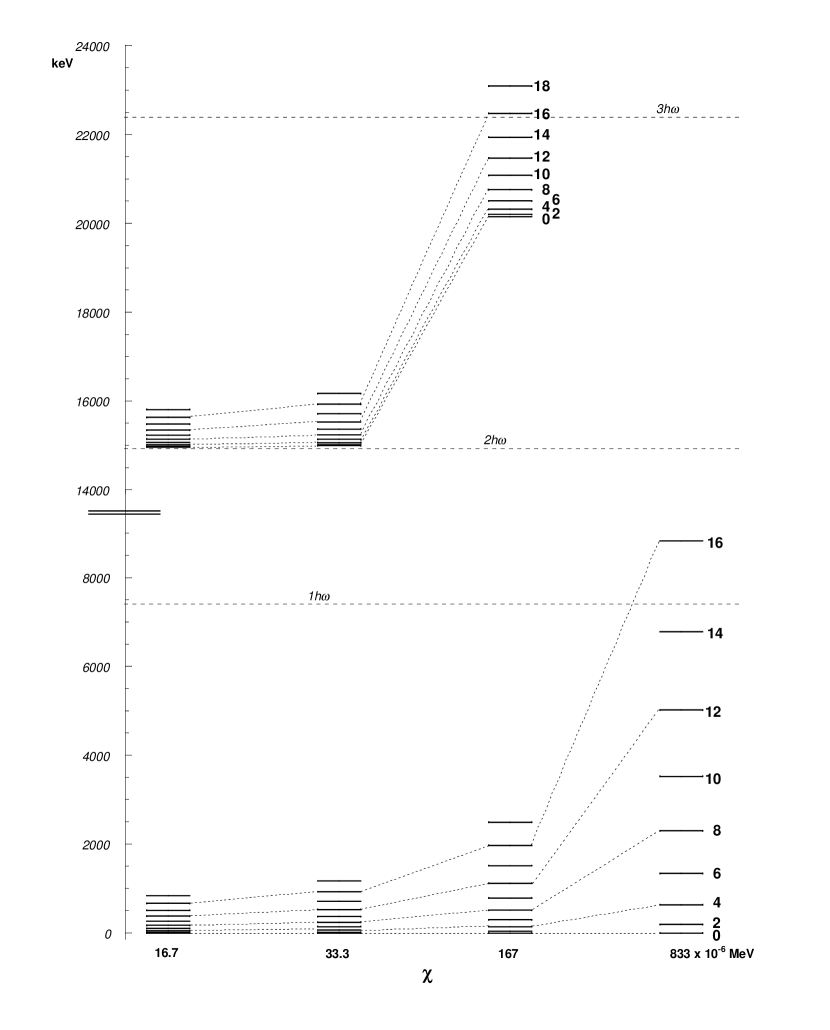
FIG. 2.: The energy spectra for various strengths of the potential. The dashed lines connect energy levels of the same angular momenta.

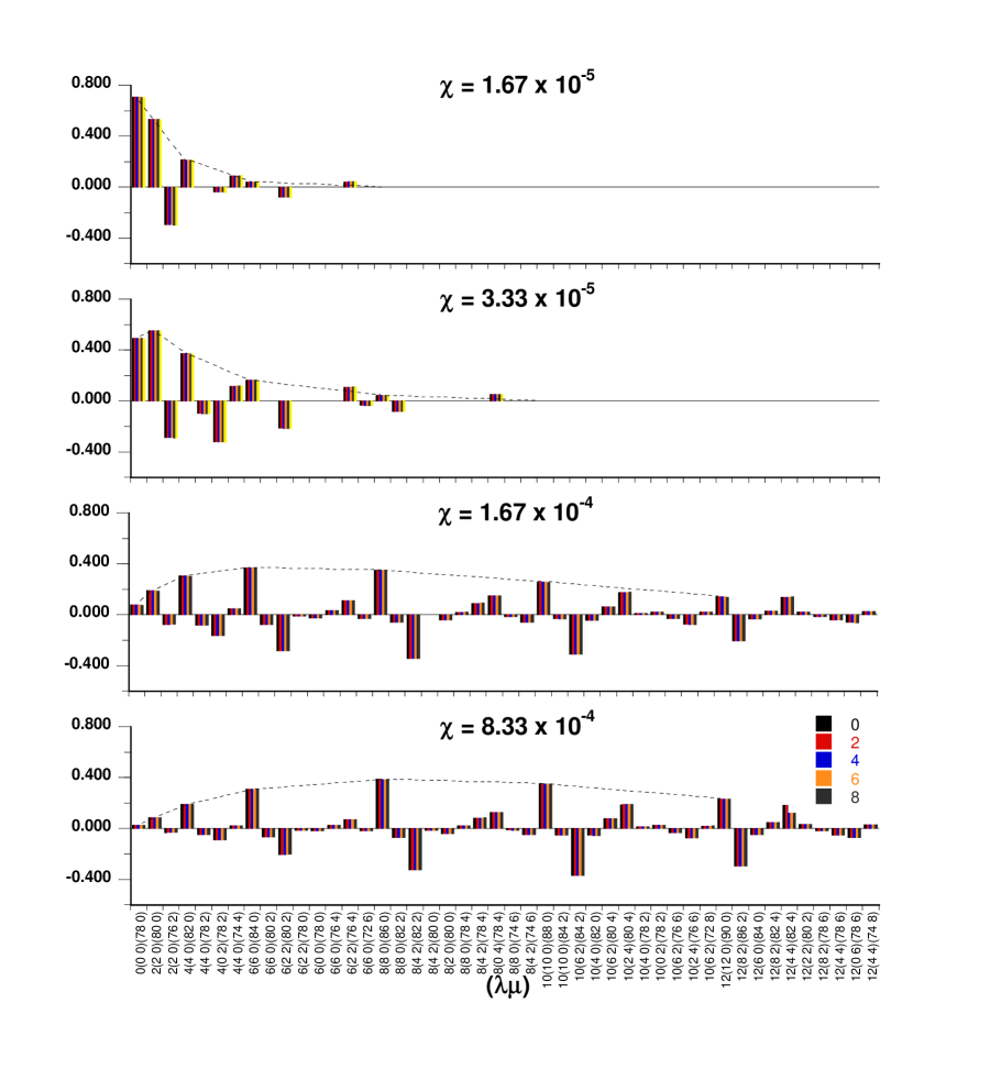
FIG. 3.: Histograms of the SU(3) amplitudes for the yrast states with variation of the strengths of the potential. The so-called stretched states are connected with dashed lines.

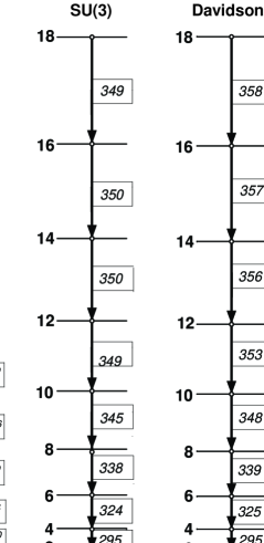
FIG. 4.: Energy spectra for experimental data, the SU(3), the symplectic-Davidson, and the rigid rotor models. The $B(E2)$ values are given inside the boxes.

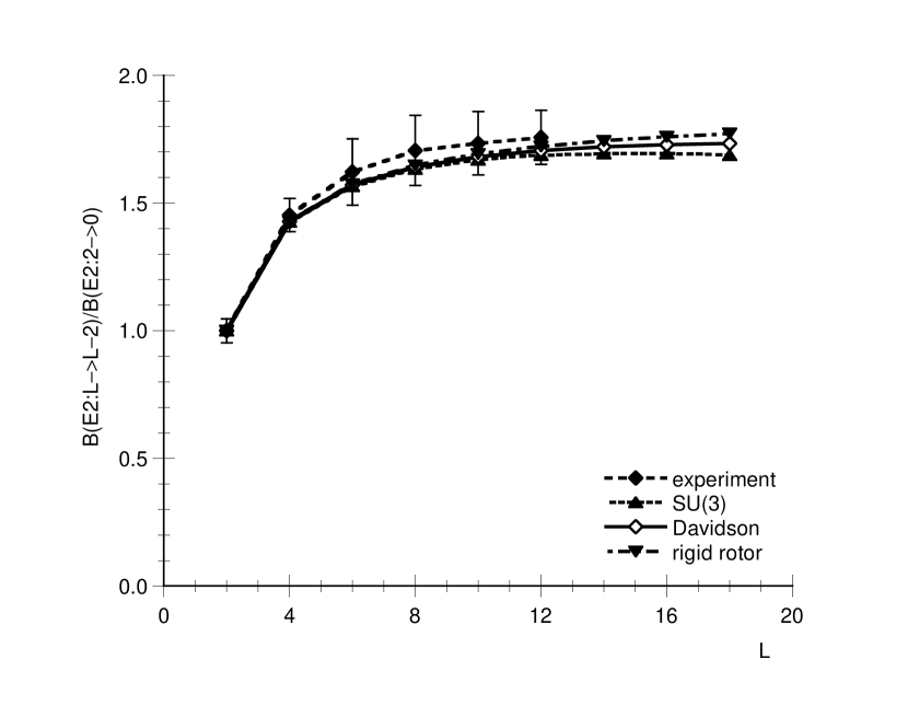
FIG. 5.: Relative $B(E2)$ values for experimental data, the SU(3), the symplectic-Davidson, and the rigid rotor models.

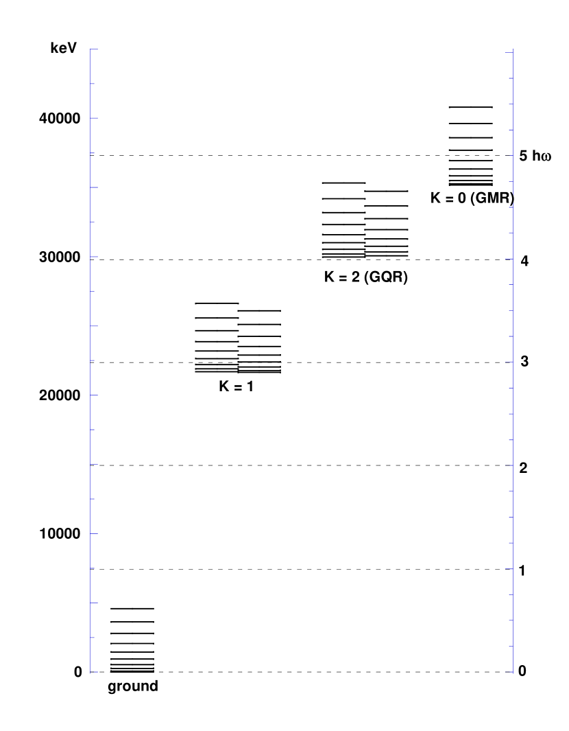
FIG. 6.: Energy spectra in the Davidson-symplectic model for the ground-state and breathing-mode (giant-beta) bands with the self-consistent parameter strength $\chi=3.33\times 10^{-4}$ MeV.

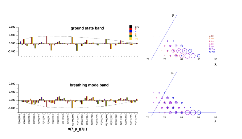
FIG. 7.: Histograms and corresonding plots on an SU(3) weight diagram of the SU(3) amplitude coefficients for the ground-state and breathing-mode (giant-beta) bands.

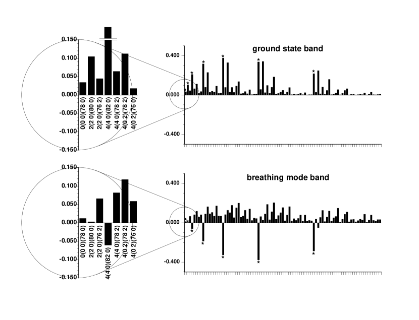
FIG. 8.: As for Fig. 7 except that only $L=0$ coefficients are plotted and the phase factor for the ground-state coefficients are set to be positive. The stretched bases are indicated by asterisks. The insets show changes of phase for the first few coefficients.

- [1] H.B.G. Casimir, Rotation of a rigid body in quantum mechanics, Dissertation, Gröningen.
- [2] G. Rosensteel and D.J. Rowe, Phys. Rev. Lett. 38, 10 (1977).
- [3] G. Rosensteel and D.J. Rowe, Ann. Phys. NY 126, 343 (1980).
- [4] P. Park, M.J. Carvalho, M.G. Vassanji, D.J. Rowe, and G. Rosensteel, Nucl. Phys. A 414, 93 (1984).
- [5] P. Rochford and D.J. Rowe, Phys. Lett. B210, 5 (1988).
- [6] D.J. Rowe, C. Bahri, and W. Wijesundera, Phys. Rev. Lett. 80, 4394 (1998).
- [7] C. Bahri, D.J. Rowe, and W. Wijesundera, Phys. Rev. C 58, 1539 (1998).
- [8] D.J. Rowe, “Quasi-Dynamical Symmetry — a new use of symmetry in nuclear physics”, in The Nucleus; New Physics for the New Millennium, ed. F.D. Smit and R. Lindsay (Plenum Press, U.K., 1999) in press.
- [9] P.M. Davidson, Proc. Roy. Soc. London 135, 459 (1932).
- [10] D.J. Rowe and C. Bahri, J. Phys. A 31, 4947 (1998).
- [11] J.P. Elliott, J.A. Evans, and P. Park, Phys. Lett. B 169, 309 (1986); J.P. Elliott, P. Park, and J.A. Evans, Phys. Lett. B 171, 145 (1986).
- [12] A. Bohr, Kgl. Danske Vidensk. Selsk. Mat.-Fyz. Medd. 26, 14 (1952); A. Bohr and B. Mottelson, Kgl. Danske Vidensk. Selsk. Mat.-Fyz. Medd. 27, 16 (1953); A. Bohr, B. Mottelson, and J. Rainwater, Rev. Mod. Phys. 48, 365 (1978).
- [13] J.P. Elliott, Proc. Roy. Soc. London A 245, 128, 562 (1958).
- [14] D.J. Rowe, J. Math. Phys. 25, 2662 (1984); D.J. Rowe, G. Rosensteel and R. Carr, J. Phys. A: Math. Gen. 17 (1984) L399; D.J. Rowe and J. Repka, J. Math. Phys. 32 (1991) 2614.
- [15] D.J. Rowe, Rep. Prog. Phys. 48, 1419 (1984).
- [16] H. Ui, Prog. Theor. Phys. 44 (1970) 153.
- [17] D.J. Rowe, P. Rochford, and J. Repka, J. Math. Phys. 29, 572 (1988).
- [18] J. Carvalho, Ph.D. thesis, Toronto (1984); R. Le Blanc, J. Carvalho, and D.J. Rowe, Phys. Lett. B140, 155 (1984).
- [19] M. Vassanji and D.J. Rowe, Nucl. Phys. A 426, 205 (1984); — A 454, 288 (1986); J. Carvalho, M. Vassanji, and D.J. Rowe, Nucl. Phys. A 466, 265 (1987); F. Arikx, J. Broeckhove, M.G. Vassanji, and D.J. Rowe, Nucl. Phys. A 511, 49 (1990); J. Carvalho, M. Vassanji, and D.J. Rowe, Phys. Lett. B 318, 273 (1993); J. Carvalho and D.J. Rowe, Nucl. Phys. A 618, 65 (1997).
- [20] M. Born and J.R. Oppenheimer. Ann. Phys. 84 (1927) 457.
- [21] G. Rosensteel, Nucl. Phys. A 341, 397 (1980).
- [22] M. Jarrio, J.L. Wood and D.J. Rowe, Nucl. Phys. A528, 409 (1991).
- [23] L.C. Biedenharn and J.D. Louck, Comm. Math. Phys. 8, 89 (1968); J.D. Louck, Am. J. Phys. 8, 89 (1968); J.D. Louck and L.C. Biedenharn, J. Math. Phys. 11, 2368 (1970).
- [24] J.P. Draayer and Y. Akiyama, J. Math. Phys. 14, 1904 (1973); Y. Akiyama and J.P. Draayer, Comp. Phys. Comm. 5, 405 (1973).
- [25] Evaluated experimental nuclear structure data ENSDF, ed. by National Nuclear Data Center, Brookhaven National Laboratory, Upton, NY 11973, USA (taken Jan. 20, 1998). Updated experimental data were obtained via telnet at bnlnd2.dne.bnl.gov.
- [26] P.J. Twin, et al., Phys. Rev. Lett. 57, 811 (1986).
- [27] C. Baktash, B. Haas, and W. Nazarewicz, Annu. Rev. Nucl. Part. Sci. 45, 543 (1995).