Numerical analysis of two-pion correlation based on a hydrodynamical model

Abstract

We will numerically investigate two-particle correlation function of CERN–SPS 158 A GeV Pb+Pb central collisions in detail based on a (3+1)-dimensional relativistic hydrodynamical model with first order phase transition. We use the Yano-Koonin-Podgoretskiĭ parametrization as well as the usual Cartesian parametrization and analyze the pair momentum dependence of HBT radii extracted from the parametrizations. We find that the interpretation of the temporal radius parameters as the time duration in YKP parametrization is not available for the hydrodynamical model where the source became opaque naturally because of expansion and surface dominant freeze-out. Finally, effect of the phase transition on the source opacity is also discussed.

I Introduction

Ultra-relativistic heavy ion collision aimed at producing the Quark-Gluon Plasma (QGP) state is one of the most attracting problems in modern nuclear-particle physics [1]. In these decades, many kinds of candidates for the signal of the production or existence of QGP are proposed. Two-particle correlation has been accepted as one of the probable observables for finding anomalous events in which QGP can be produced, because of the naive speculation that an extremely huge hot region will be produced if phase transition occurs [2, 3]. In quantum optics, estimating source size through quantum correlation of emitted particles is a well-established method called the Hanbury-Brown Twiss(HBT) effect [4, 5].

Usually, parameters obtained from the Gaussian fit of the correlation functions are regarded as a radius of the particle source (HBT radius). However, if the source is not static, the interpretation of the Gaussian parameter is not straightforward [6, 7]. In the case of ultra-relativistic heavy ion collision, in addition to the highly dynamical properties, many kinds of experimental limitations, such as rapidity windows, make the situation more complicated. In the recent analyses, there exist two ways of parametrization in the Gaussian fit of the two-particle correlation function; one is Cartesian parametrization [8, 9], and the other is Yano-Koonin-Podgoretskiĭ parametrization [10, 11, 12]. In both parametrizations, we can obtain their respective “size” of particle sources. However different parametrization gives different values and interpretation of their values is not clear enough.

In this paper we evaluate two-particle correlation functions of pion based on a hydrodynamical model with phase transition. Parameters in the hydrodynamical model are so tuned as to reproduce single particle distributions of CERN 158 A GeV Pb+Pb collisions [13]. Comparing the source size obtained through correlation and freeze-out hypersurface of the hydrodynamical model, we investigate the physical meaning of the HBT radii in both parametrizations. The opaque property [14] of the source is also analyzed based on a hydrodynamical model. In a hydrodynamical model, particle emission takes place on the freeze-out hypersurface which is thin but not an instant in time. Expansion of the fluid also should naturally occur. Hence, the apparent opaque property of the freeze-out hypersurface is not trivial. The influence of first order phase transition is also investigated.

In section II, we make a brief introduction to the hydrodynamical model with phase transition. In section III, we formulate two-particle correlation functions. Transverse momentum dependence and rapidity dependence of source parameters are discussed in Section IV and V, respectively. Section VI is devoted to the concluding remarks.

II Hydrodynamical Model

Focusing our discussion to the central collisions, we may assume cylindrical symmetry to the system and introduce cylindrical coordinates $\tau$, $\eta$, $r$ and $\phi$ instead of the usual Cartesian coordinates $x$, $y$, $z$ and $t$, where,

$$t = \tau\cosh\eta,$$ (2)

$$z = \tau\sinh\eta,$$ (3)

$$x = r\cos\phi,$$ (4)

$$y = r\sin\phi.$$ (5)

The four velocities of the fluid $U^{\mu}$ is given as,

$$U^{t} = U^{\tau}\cosh\eta+U^{\eta}\sinh\eta,$$ (7)

$$U^{z} = U^{\tau}\sinh\eta+U^{\eta}\cosh\eta,$$ (8)

$$U^{x} = U^{r}\cos\phi+U^{\phi}\sin\phi,$$ (9)

$$U^{y} = U^{r}\sin\phi-U^{\phi}\cos\phi.$$ (10)

Taking the constraint, $U^{\mu}U_{\mu}=1$, and cylindrical symmetry into account, $U^{\mu}$ can be represented with two variables $Y_{\text{L}}$ and $Y_{\text{T}}$ [15],

$$U^{\tau} = \cosh Y_{\text{T}}\cosh(Y_{\text{L}}-\eta),$$ (12)

$$U^{\eta} = \cosh Y_{\text{T}}\sinh(Y_{\text{L}}-\eta),$$ (13)

$$U^{r} = \sinh Y_{\text{T}},$$ (14)

$$U^{\phi} = 0.$$ (15)

As is well known, the relativistic hydrodynamical equation is given as

$$\partial_{\mu}T^{\mu\nu}=0,$$ (16)

and the energy momentum tensor of perfect fluid is given by

$$T^{\mu\nu}=EU^{\mu}U^{\nu}-P(g^{\mu\nu}-U^{\mu}U^{\nu})$$ (17)

where $E$ and $P$ are energy density and pressure, respectively, and the metric tensor $g^{\mu\nu}$ is $g^{\mu\nu}$ = diag.$(1,-1,-1,-1)$. In a hydrodynamical model, thermodynamical quantities such as $E$ and $P$ are treated as local quantities through temperature $T=T(x^{\mu})$.

In order to solve the above hydrodynamical equation, we need an equation of state. In this paper, we adopt the bag model equation of state as the simplest model for the first order QCD phase transition. In the bag model, thermodynamical quantities below the phase transition temperature correspond to a massive hadronic gas. On the other hand, in the high temperature phase, thermodynamical quantities are given by a massless QGP gas with bag constant $B$. In this paper, we assume pions and kaons in the hadronic phase and u-, d-, s-quarks and gluons in the QGP phase. Putting the phase transition temperature, $T_{\text{c}}=160$ MeV, into the condition of pressure continuity, we can obtain the bag constant as $B=412$ MeV/fm³.

At the phase transition temperature $T_{\text{c}}$, pressure $P$ is continuous but other quantities such as energy density $E$ and entropy density $S$ have discontinuity as a function of temperature. We parameterize these quantities during the phase transition by using the volume fraction $\lambda$ [16, 17]. We assume that thermodynamical quantities at $T=T_{\text{c}}$ are given as the functions of the space-time point through $\lambda(x^{\mu})$,

$$E(\lambda) = \lambda E_{\text{QGP}}(T_{\text{c}})+(1-\lambda)E_{\text{HAD}}(T_{\text{c}}),$$ (19)

$$S(\lambda) = \lambda S_{\text{QGP}}(T_{\text{c}})+(1-\lambda)S_{\text{HAD}}(T_{\text{c}}),$$ (20)

where $0\leq\lambda(x^{\mu})\leq 1$. This parametrization enables us to solve the hydrodynamical equation easily.

We consider that the hadronization process occurs at freeze-out temperature $T_{\text{f}}$ = 140 MeV. In the evaluation of the one-particle distribution in a hydrodynamical model, the Cooper-Frye formula [18] is often used, however, there exist several delicate matters on the treatment of freeze-out hypersurface based on this formula [19, 20]. In this paper, we analyze not only one-particle distribution but also two-particle distribution, hence, we adopt another type of the simplest formula which enables us to extend two-particle distributions straightforward,

$$\frac{d^{3}\Delta N_{i}}{d{\bf p}^{3}}=\frac{U_{\mu}p^{\mu}}{\sqrt{{\bf p}^{2}+m^{2}_{i}}}\frac{1}{\exp\left(\frac{U_{\nu}p^{\nu}}{T}\right)-1}\frac{U_{\lambda}d\sigma^{\lambda}}{(2\pi)^{3}},$$ (21)

where $p^{0}=\sqrt{{\bf p}^{2}+m_{i}^{2}}$ and the subscript $i$ stands for pion or kaon. Integrating (21) on the freeze-out hypersurface $\Sigma$, we obtain the rapidity distribution,

$$\frac{dN_{i}}{dY}=\int_{\Sigma}\frac{U_{\mu}p^{\mu}}{\exp\left(\frac{U_{\nu}p^{\nu}}{T}\right)-1}\frac{U_{\lambda}d\sigma^{\lambda}p_{T}dp_{T}d\phi}{(2\pi)^{3}},$$ (22)

and the transverse mass distribution,

$$\frac{1}{m_{T}}\frac{dN_{i}}{dm_{T}}=\int_{\Sigma}\frac{U_{\mu}p^{\mu}}{\exp\left(\frac{U_{\nu}p^{\nu}}{T}\right)-1}\frac{U_{\lambda}d\sigma^{\lambda}dYd\phi}{(2\pi)^{3}}.$$ (23)

In a previous paper, we have already analyzed one-particle distribution of hadrons by using results of our hydrodynamical model and compared it to the data at CERN SPS experiment [13]. The detailed structure of space-time evolution and particle distribution is discussed in the Appendix.

III Two-Pion Correlation Function

Two-particle correlation function is defined as

$$C({\bf k_{1}},{\bf k_{2}})=\frac{W({\bf k_{1}},{\bf k_{2}})}{W({\bf k_{1}})W({\bf k_{2}})}\,,$$ (24)

where $W({\bf k})$ and $W({\bf k_{1}},{\bf k_{2}})$ are one-particle distribution $E_{k}~{}dN/d^{3}{\bf k}$ and two-particle distribution $E_{k_{1}}E_{k_{2}}~{}dN/d^{3}{\bf k_{1}}d^{3}{\bf k_{2}}$, respectively. Assuming that the source is completely chaotic, for simplicity, the two-particle correlation function for identical bosons (i.e.,pions) is rewritten as [21]

$$C({\bf k_{1}},{\bf k_{2}})=1+\frac{|I({\bf k_{1}},{\bf k_{2}})|^{2}}{W({\bf k_{1}})W({\bf k_{2}})},$$ (25)

where

$$I({\bf k_{1}},{\bf k_{2}})=\int_{\Sigma}U_{\mu}d\sigma^{\mu}\,e^{i(k_{1}-k_{2})_{\nu}x^{\nu}}\sqrt{F({\bf k_{1}},x)F({\bf k_{2}},x)}\,,$$ (26)

and

$$F({\bf k},x)=\frac{1}{(2\pi)^{3}}\frac{U_{\mu}k^{\mu}}{E_{k}}\frac{1}{\exp(\frac{U_{\nu}k^{\nu}}{T_{f}})-1}\,.$$ (27)

As usual, we introduce the average momentum $K^{\mu}=\frac{1}{2}(k_{1}^{\mu}+k_{2}^{\mu})$ and the relative momentum $q^{\mu}=k_{1}^{\mu}-k_{2}^{\mu}$ of two particles. Taking an approximation that ${\bf k_{1}}\simeq{\bf k_{2}}\simeq{\bf K}$ in Eq.(25), the two-particle correlation function $C({\bf k_{1}},{\bf k_{2}})$ can be expressed as [8, 22]

$$C(q^{\mu},K^{\mu})\simeq 1+\frac{|\int d^{4}x\,e^{iq_{\mu}x^{\mu}}\,S(x^{\mu},K^{\mu})|^{2}}{|\int d^{4}x\,S(x^{\mu}.K^{\mu})|^{2}},$$ (28)

where $S(x^{\mu},K^{\mu})$ is the source function,

$$S(x^{\mu},K^{\mu})=\int_{\Sigma}U_{\mu}(x^{\prime})d\sigma^{\mu}(x^{\prime})E_{K}F({\bf K},x^{\prime})\delta^{4}(x-x^{\prime})\ .$$ (29)

Furthermore, expanding $e^{iq_{\mu}x^{\mu}}$ in Eq.(28) with $q_{\mu}x^{\mu}\ll 1$, we can obtain the simple expression

$$C(q^{\mu},K^{\mu})-1\approx 1+\langle q_{\mu}x^{\mu}\rangle^{2}-\langle(q_{\mu}x^{\mu})^{2}\rangle,$$ (30)

with $\langle A(x^{\mu})\rangle$ being weighted average ,

$$\langle A(x^{\mu})\rangle\equiv\frac{\int d^{4}x\,A(x^{\mu})S(x^{\mu},K^{\mu})}{\int d^{4}x\,S(x^{\mu},K^{\mu})}\,.$$ (31)

Consequently, we can recognize the two-particle correlation function as the second order moment of $q_{\mu}x^{\mu}$ with the weight of $S(x^{\mu},K^{\mu})$. Because of the on-shell property of final particles, the relative momentum $q_{\mu}$ has three independent components. Choosing the three independent components of $q^{\mu}$ in an appropriate manner, we can obtain meaningful information on the space-time structure of the particle source.

In the estimation of the source sizes from the two-particle correlation function (25), two types of Gaussian parametrizations[11] are widely used. One is the Cartesian parametrization, including the outward-longitudinal cross term [9], and the other is so called Yano-Koonin-Podgoretskiĭ parametrization [10, 12]. We take the z-axis in the direction of the collision and the x-axis parallel to the transverse component of the average momentum $K^{\mu}=(K^{0},K_{T},0,K_{L})$, as usual. Then the z-axis, x-axis and y-axis correspond to so-called “longitudinal”, “outward” and “sideward” directions, respectively.

In the Cartesian parametrization, the three independent components of the relative momentum $q_{\mu}$ are $(q_{x},q_{y},q_{z})=(q_{\text{out}},q_{\text{side}},q_{\text{long}})$. In this parametrization, the fitting function with the average momentum $K^{\mu}$ is given as

$$C(q^{\mu},K^{\mu})=1+\lambda\exp\left[-R_{\text{side}}^{2}(K^{\mu})q_{\text{side}}^{2}-R_{\text{out}}^{2}(K^{\mu})q_{\text{out}}^{2}-R_{\text{long}}^{2}(K^{\mu})q_{\text{long}}^{2}-2R_{\text{ol}}^{2}(K^{\mu})q_{\text{out}}q_{\text{long}}\right].$$ (32)

There are four fitting parameters in Eq.(32), namely, $R_{\text{side}}$, $R_{\text{out}}$, $R_{\text{long}}$ and $R_{\text{ol}}$, which are so-called HBT radii. As for $\lambda$, we fix its value one because we have assumed chaotic sources.

In this parametrization, the meaning of these HBT radii, which is given through Eq.(30), depends on the observer’s longitudinal frame. The coordinate system where $\beta_{l}=K_{L}/K^{0}=0$ is called longitudinal co-moving system (LCMS), and on this system, the interpretation becomes very simple [8],

$$R_{\text{side}}^{2}\quad = \quad\left\langle\tilde{y}^{2}\right\rangle,$$ (34)

$$R_{\text{out}}^{2}\quad = \quad\left\langle(\tilde{x}-\beta_{\bot}\tilde{t})^{2}\right\rangle,$$ (35)

$$R_{\text{long}}^{2}\quad = \quad\left\langle\tilde{z}^{2}\right\rangle,$$ (36)

$$R_{\text{ol}}^{2}\quad = \quad\left\langle(\tilde{x}-\beta_{\bot}\tilde{t})\tilde{z}\right\rangle,$$ (37)

where $\tilde{x}=x-\langle x\rangle$ and $\beta_{\bot}=K_{T}/K^{0}$. It is clearly seen that these radii mix spatial and temporal components. Therefore, from this parametrization it is not easy to extract accurately physical information such as emission duration [12].

In the Yano-Koonin-Podgoretskiĭ (YKP) parametrization, the three independent components of relative momentum are chosen as $q_{\bot}=\sqrt{q_{\text{side}}^{2}+q_{\text{out}}^{2}}$, $q_{l}=q_{\text{long}}$ and $q^{0}=E_{1}-E_{2}$. The fitting function is given as [12]

$$C(q^{\mu},K^{\mu})=1+\lambda\exp\left\{-R_{\bot}^{2}(K^{\mu})q_{\bot}^{2}-R_{\|}^{2}(K^{\mu})\left[q_{l}^{2}-(q^{0})^{2}\right]-\left[R_{0}^{2}(K^{\mu})+R_{\|}^{2}(K^{\mu})\right][q_{\mu}u^{\mu}(K^{\mu})]^{2}\right\},$$ (38)

where $u(K^{\mu})=\gamma(K^{\mu})(1,0,0,v(K^{\mu}))$, and $\gamma(K^{\mu})=1/\sqrt{1-v^{2}(K^{\mu})}$. We fixed $\lambda=1$ as well as in the Cartesian parametrization. Hence, the fitting parameters are $R_{\bot}$, $R_{0}$, $R_{\|}$ and the so-called Yano-Koonin-Podgoretskiĭ velocity $v$ which appears in the four-velocity $u^{\mu}$. The first three parameters are the HBT radii that are invariant under longitudinal boosts. This is one of the most important properties of the YKP parametrization. The four-velocity $u^{\mu}$ has a longitudinal component only, and the Yano-Koonin-Podgoretskiĭ velocity $v$ can be interpreted as the longitudinal source velocity [12]. The interpretation of the HBT radii in the YKP parametrization can be given in the same manner as in Cartesian parametrization. Denoting deviation as $(\Delta A)^{2}=\left\langle(A-\langle A\rangle)^{2}\right\rangle$ and

$$A = (\Delta t)^{2}-\frac{2}{\beta_{\bot}}\langle\tilde{x}\tilde{t}\rangle+\frac{1}{\beta_{\bot}^{2}}\left[(\Delta x)^{2}-(\Delta y)^{2}\right],$$ (40)

$$B = (\Delta z)^{2}-\frac{2\beta_{\|}}{\beta_{\bot}}\langle\tilde{x}\tilde{z}\rangle+\frac{\beta_{\|}^{2}}{\beta_{\bot}^{2}}\left[(\Delta x)^{2}-(\Delta y)^{2}\right],$$ (41)

$$C = \langle\tilde{z}\tilde{t}\rangle-\frac{\beta_{\|}}{\beta_{\bot}}\langle\tilde{t}\tilde{x}\rangle-\frac{1}{\beta_{\bot}}\langle\tilde{z}\tilde{x}\rangle+\frac{\beta_{\|}}{\beta_{\bot}^{2}}\left[(\Delta x)^{2}-(\Delta y)^{2}\right],$$ (42)

the HBT radii and Yano-Koonin-Podgoretskiĭ velocity are expressed as follows [12] :

$$v(K^{\mu}) = \frac{A+B}{2C}\left[1-\sqrt{1-\left(\frac{2C}{A+B}\right)^{2}}\right]$$ (44)

$$R_{\bot}^{2}(K^{\mu}) = (\Delta y)^{2}$$ (45)

$$R_{0}^{2}(K^{\mu}) = A-vC$$ (46)

$$R_{\|}^{2}(K^{\mu}) = B-vC.$$ (47)

Even in the YKP parametrization, $R_{\bot}$ directly corresponds to transverse size. In the Yano-Koonin-Podgoretskiĭ(YKP) frame which is defined by $v=0$, these expressions (45-47) become very simple,

$$R_{\bot}^{2}(K^{\mu}) = (\Delta y)^{2}\ ,$$ (49)

$$R_{0}^{2}(K^{\mu}) = (\Delta t)^{2}-\frac{2}{\beta_{\bot}}\langle\tilde{x}\tilde{t}\rangle+\frac{1}{\beta_{\bot}^{2}}\left[(\Delta x)^{2}-(\Delta y)^{2}\right]\ ,$$ (50)

$$R_{\|}^{2}(K^{\mu}) = (\Delta z)^{2}-\frac{2\beta_{\|}}{\beta_{\bot}}\langle\tilde{x}\tilde{z}\rangle+\frac{\beta_{\|}^{2}}{\beta_{\bot}^{2}}\left[(\Delta x)^{2}-(\Delta y)^{2}\right].$$ (51)

The values of these quantities do not change because they are invariant under longitudinal boosts. But now the $\langle\cdots\rangle$ is taken in the YKP frame. It has been shown that the last two terms in Eqs.(50) and (51) can be considered as a small correction within some class of the thermal model [12]. Hence, the three HBT radii can be considered to measure the “source size” directly. Specifically, $R_{0}$ measures the emission duration on which, according to a naive expectation, the effect of first order phase transition may be observed. Of course, it is not clear that this interpretation works well even in the hydrodynamical model.

IV Transverse Momentum Dependence of Source Parameters

In this section, we will discuss the dependence of HBT radii on the transverse momentum $K_{T}$. Because of the lack of experimental data with fixed average momenta, in order to make a comparison with the experimental data, we integrate the distribution functions in (25) with respect to average momenta and

$$C(q^{\mu};K_{T}) = 1+\frac{\int dK_{L}\,|I({\bf k_{1}},{\bf k_{2}})|^{2}}{\int dK_{L}\,W({\bf k_{1}})W({\bf k_{2}})},$$ (53)

$$C(q^{\mu};Y) = 1+\frac{\int K_{T}dK_{T}\,|I({\bf k_{1}},{\bf k_{2}})|^{2}}{\int K_{T}dK_{T}\,W({\bf k_{1}})W({\bf k_{2}})},$$ (54)

is used.

Figure 1 shows the dependence of Cartesian HBT radii on the average transverse momentum $K_{T}$. Closed circles stand for our numerical results obtained from the correlation function (53) through the fitting function (32). Experimental results taken from NA49 preliminary data [23] are plotted as open circles. Our results almost agree with the experimental data. However, we get the HBT radii a little larger than experimental results at high $K_{T}$. In the upper left figure of Fig. 1, though experimental $R_{\text{side}}$ becomes smaller at larger $K_{T}$, this tendency appears only weakly in our simulation. This $K_{T}$ dependence of $R_{\text{side}}$ can be explained by the existence of strong transverse flow [7] and contributions from resonance decay [25]. Hence, the differences between our calculation and experimental results might be caused by the simplification that neglected the resonance decay.

As we discussed in the previous section, a simple interpretation is not available to HBT radii in the Cartesian parametrization; investigating the source parameters based on the YKP parametrization is important. Figure 2 shows the dependence of YKP radii on average transverse momentum $K_{T}$. As mentioned in Sec. III, in the YKP parametrization, the HBT radii are expected to stand for longitudinal invariant “source size”. In Fig. 2, closed circles stand for YKP radii obtained from the correlation function (53) through fitting based on Eq.(38). Solid lines stand for the space-time extensions of freeze-out hypersurface evaluated from the right-hand side of Eq.(49)-(51). These quantities are expected to agree with our HBT radii because in our calculation we consider only thermal pions [26]. Dotted lines shows “source sizes” ($\Delta z$ for $R_{\|}$ and $\Delta t$ for $R_{0}$) calculated from the second order moment, i.e., first terms only in the right-hand side of Eq.(50)-(51). In the calculation of space-time extensions and “source sizes”, average momenta are fixed at the central value of the integration range. NA49 experimental data [24] are plotted as open circles.

The upper figure shows the dependence of the transverse source radii $R_{\bot}$ on $K_{T}$. As we have already discussed, $R_{\bot}$ in the YKP parametrization is the same as $R_{\text{side}}$ in the Cartesian parametrization. The difference between the space-time extension and YKP radius $R_{\bot}$ is about 0.5fm.

The middle part of Fig. 2 shows the dependence of longitudinal source radius $R_{\|}$ on $K_{T}$. Our result from the fit is consistent with both the experiment and space-time extension. Furthermore, the “source size” $\Delta z$ also agrees with the space-time extension. Hence, the usual interpretation of $R_{\|}$ in the YKP parametrization works well in our calculation.

The lower figure shows the dependence of the temporal source parameter $R_{0}$ on $K_{T}$. Our results from the fit are a few fm smaller than experimental results and become smaller as $K_{T}$ increases. The space-time extension calculated from Eq.(50) shows similar behavior in $K_{T}$ but quantitatively agreement is not so good at large $K_{T}$. Because of the on-shell condition, the available $q^{\mu}$ region is limited and a great ambiguity in fitting process can occur. For example, $R_{0}^{2}$ sometimes tends to become negative if we take the most likely values without any restriction to $R_{0}^{2}$. However, it becomes small but positive definite values if we impose the restriction on $R_{0}^{2}$ to be positive. As for the “time duration” $\Delta t$, though it agrees with $R_{0}$ at low $K_{T}$, it becomes larger than $R_{0}$ at large $K_{T}$. Hence, the interpretation that $R_{0}$ measures the time duration directly in the YKP parametrization is not correct in this region. This can be explained by the effect of “source opacity” [14], which will be discussed later. On the other hand, the values of $R_{0}$ and $\Delta t$ are about 2-3 fm, obviously smaller than $R_{\bot}$, $R_{\|}$. Hence, we can say that clear evidence of the first order phase transition does not appear in the time duration. It was already pointed out that the large time duration (or longer lifetime) might not occur for Bjorken-type scaling, the initial condition we used [2, 27].

The “opaque” source emits particles dominantly from the surface and the “transparent” source emits from whole region. Whether the “real” source is opaque or transparent is an interesting problem [28]. Aiming for this point, we analyze the source function $S(x^{\mu},K^{\mu})$ for $K_{T}=450$ MeV and $Y_{\pi\pi}=4.15$. Figure 3 shows the source function as a function of transverse coordinates $x$ and $y$. Here the source function is integrated in the temporal and longitudinal coordinates, $\bar{S}_{T}(x,y)=*\int dz\,dt\,S(x^{\mu},K^{\mu})$, and normalized on the transverse plane as $\int dx\,dy\,\bar{S}_{T}(x,y)=1$. In this figure, emitted pions have only $x$ component of momentum. Figure 3 clearly shows that pions are emitted mostly from the crescent surface region and the source is thinner in the $x$-direction than in the $y$-direction. This is the typical property of the opaque source. Therefore, the difference between $\Delta x$ and $\Delta y$, that is, the difference of space-time extensions $(\Delta x)^{2}-(\Delta y)^{2}$ is a good measure of the opaque property[29].

Figure 4 shows the dependence of the second and third terms in Eq.(50) on $K_{T}$. The third term $((\Delta x)^{2}-(\Delta y)^{2})/\beta_{\bot}^{2}$ has a large negative contribution to $R_{0}$ at a large $K_{T}$ region, while the contribution from the second term $-2\langle\tilde{x}\tilde{t}\rangle/\beta_{\bot}$ is not so large. Hence we may not consider the third term as a small correction to $(\Delta t)^{2}$ and this is the reason why the simple interpretation of $R_{0}$ in the YKP parametrization is not available in our calculation. A simple model analysis [29] has shown the contradictory result that $R_{0}$ diverges to $-\infty$ as $K_{T}\rightarrow 0$ ($\beta_{\bot}\rightarrow 0$) for the opaque source. This is due to the tendency of the denominator of the third term in Eq.(50) to go to zero as $K_{T}\rightarrow 0$ while the numerator is kept as finite. However, this divergence does not occur in our model because the numerator, $(\Delta x)^{2}-(\Delta y)^{2}$, goes to 0 as $K_{T}\rightarrow 0$.

Figure 5 also shows the source function $\bar{S}_{T}(x,y)$ with the artificially neglected transverse flow. In order to see the effect of transverse flow on the source function, here we put the transverse flow velocity $U^{r}=0$ by hand. In this case, the source function $\bar{S}_{T}(x,y)$ is almost proportional to the space-time volume of freeze-out hypersurface projected onto the transverse plane, and the azimuthal symmetry of the source function is restored as shown in Fig. 5. As a result, the measure of the source opacity, $(\Delta x)^{2}-(\Delta y)^{2}$, vanishes. Although particle emission from the inside is less than that from the surface; the source is not opaque in this sense. When the transverse flow exists, the source function is deformed by the thermal Boltzmann factor $\exp(\cosh Y_{T}\cos\phi\,K_{T}/T_{f})$ and in our simulation the transverse flow rapidity, $Y_{T}$, is almost proportional to $r$ as shown in Fig. 20. Consequently, the number of emitted particles in $x$-direction is increased for the positive $x$ region ($\cos\phi>0$), especially at the surface, because of the behavior of $Y_{T}$, and the number is decreased for the negative $x$ region ($\cos\phi<0$). This flow effect deforms surface dominant distribution in Fig. 5 to the crescent shape. This is the main reason why the source is opaque in our model. Though in the recent experimental result, $R_{0}$ is larger than expected for the opaque source. According to the scenario as discussed in Ref.[27], the phase transition may cause a large time duration for the opaque source. However, in our hydrodynamical model, we assumed the first order phase transition, but the time duration $\Delta t$ does not become large enough to reproduce the experiment.

In order to discuss the effects of the phase transition on the source opacity, we sliced the source function $S_{T}(x,y)$ by the freeze-out proper time $\tau$ and show the source functions for each proper time in Fig. 6,7. Figures 6(a)-7(j) show the same quantity as Fig. 3, but they are not normalized. Integral $N=\int dx\,dy\,S_{T}(x,y)$ should be considered as the number of particles. Figures 6(a)-6(f) clearly show most particles are emitted from a thin surface. The measure of the source opacity $(\Delta x)^{2}-(\Delta y)^{2}$ evaluated for Figs. 6(b)-7(h) indicates extremely opaque property. For these sources, the YKP parametrization cannot be used because the YKP velocity becomes imaginary (i.e., $A+B<2C$ in Eq.(44)) [29]. Figure 6(a) shows strong surface emission, but this source does not show the source opacity because the transverse flow is very weak at the early stage of evolution. $(\Delta x)^{2}-(\Delta y)^{2}$ is negative throughout Fig. 6,7. As discussed in the Appendix, if first order phase transition exists, a flat-top structure appears in temperature distribution (Fig. 18) which corresponds to a large region caused by latent heat released at phase transition. This equi-temperature region reaches freeze-out temperature almost simultaneously and makes a filled source function Fig. 7(j). Hence, the existence of phase transition weakens the source opacity.

V Rapidity Dependence of Source Parameters

In this section, we discuss the pair rapidity $Y_{\pi\pi}$ dependence of YKP radii. The upper figure of Fig. 8 shows the $R_{\bot}$, which is consistent with the experimental result. It is similar to the case of $K_{T}$ dependence; our result of $R_{0}$ shown in the lowest figure becomes smaller as $Y_{\pi\pi}$ increases and our $R_{0}$ does not agree with $\Delta t$. This departure also can be explained as the result of source opacity. The middle figure stands for $R_{\|}$, which shows a similar tendency as the experimental results. Source size $\Delta z$ is almost the same as the space-time extension $R_{\|}$ (47). Hence the interpretation in the YKP parametrization is applicable to our model. The disagreement of $R_{\|}$ with the experiment is due to smaller longitudinal source width at larger $Y_{\pi\pi}$. In Fig. 9, we can see that the width of the source function $\Delta\eta=\sqrt{\langle\eta^{2}\rangle-\langle\eta\rangle^{2}}$ for $\eta$-direction becomes smaller as $Y_{\pi\pi}$ increases. As shown in Fig.11, this property does not appear in a Gaussian source model [8] where the source function is given as

$$S_{g}(x^{\mu},K^{\mu})=\frac{m_{T}\cosh(\eta-Y_{\pi})}{(2\pi)^{3}\,\sqrt{2\pi(\delta\tau)^{2}}}\exp\left[-\frac{K^{\mu}U_{\mu}}{T}-\frac{(\tau-\tau_{0})^{2}}{2(\delta\tau)^{2}}-\frac{r^{2}}{2R^{2}}\right]G(\eta),$$ (55)

where

$$G(\eta)=\exp\left[-\frac{(\eta-\eta_{0})^{2}}{2(\delta\eta)^{2}}\right].$$ (56)

Of course, a small $\Delta\eta$ does not always mean a small $\Delta z$ in general, because $z$ is given as $z=\tau\sinh\,\eta$. However, in the case where freeze-out takes place almost at some fixed $\tau$, $\Delta z$ is regarded as proportional to $\Delta\eta$. And this case can be applied to our model, because for most of the particles, the freeze-out occurs at the latest stage ($\tau\sim 10$ or 11) as shown in Fig. 10. The small width of the source function in our model is due to a non-Gaussian feature of $\eta$-dependence of a geometric factor of the source function, which corresponds to $G(\eta)$ in the Gaussian source model. Figure 12 shows the corresponding normalized geometric factor for the freeze-out hypersurface in our model; the geometric factor has a central plateau region. Non-Gaussian type source function comes from both initial temperature distribution and longitudinal flow. A deformed Boltzmann factor makes the source function narrower in a high $Y_{\pi\pi}$ region. This feature is not only in a hydrodynamical model but also appears in thermal source models with a non-Gaussian geometric factor. In order to see the effect clearly, we replace $G(\eta)$ in Eq.(55) with the modified geometric factor $\tilde{G}(\eta)$. The solid line in Fig.12 denotes the modified geometric factor $\tilde{G}(\eta)$ obtained by fitting the geometric factor for our model through

$$\tilde{G}(\eta)=\exp\left[-\frac{(|\eta|-\eta_{0})^{2}}{2(\delta\eta)^{2}}\theta(|\eta|-\eta_{0})\right].$$ (57)

Using the above $\tilde{G}(\eta)$ in Eq.(55) instead of $G(\eta)$, the same source function as in Fig. 11 is evaluated, and the result is shown in Fig. 13. We can see that the width of the source function becomes narrower at a high $Y_{\pi\pi}$ region than a low $Y_{\pi\pi}$ region in the figure. Hence, we can say that the strong $Y_{\pi\pi}$ dependence of $R_{\|}$ comes from the geometric structure of the pion source in the rapidity space.

Figure 14 shows pair rapidity $Y_{\pi\pi}$ dependence of the YKP rapidity and the longitudinal expansion velocity. In our calculation, we used Eq.(38) where $Y_{\text{YKP}}$ is derived by using the YKP velocity $v$, which is given as

$$Y_{\text{YKP}}=\frac{1}{2}\ln\frac{1+v}{1-v}+Y_{\text{cm}}.$$ (58)

The dashed line stands for the infinite boost-invariant source. The departure between the solid line and the dotted line indicates that the failure of the simple interpretation of YKP velocity, which might be caused opacity of the source. The experimental results seem to be consistent with the infinite boost-invariant source except for the high rapidity region. Our results are much smaller than the boost-invariant model, as if our model contradicts the boost-invariance. Figure 15 shows average longitudinal rapidity $\langle Y_{L}\rangle$ as a function of longitudinal coordinate $\eta$ for slow ($Y_{\pi\pi}=3.4$) particles and fast ($Y_{\pi\pi}=4.9$) particles where $K_{T}$ is fixed at 150 MeV. We can clearly see $\langle Y_{L}\rangle=\eta$ for both cases. Figure 19 shows that $Y_{L}-\eta$ is positive for small $\tau$ but is negative in a later stage of the space-time evolution. Consequently, average rapidity $\langle Y_{L}\rangle$ is almost the same as $\eta$. Hence there must be another reason why $Y_{\text{YKP}}$ shows non-boost-invariant behavior. By making use of the source model, the result of the boost-invariant source is obtained by $\delta\eta\rightarrow\infty$ in Eq.(55). For the finite but large enough $\delta\eta$, the peak of the source function is only slightly shifted from $\eta=Y_{\pi\pi}$, which is the peak of the Boltzmann factor $\exp(-m_{T}\cosh(\eta-Y_{\pi\pi})/T)$. But for the small $\delta\eta$, a large shift will occur. Hence, the small $Y_{\text{YKP}}$ reflects the finite size effect rather than longitudinal expansion.

VI Concluding Remarks

In this paper, with the use of the numerical simulation for the CERN-SPS 158 A GeV Pb+Pb collisions based on a relativistic hydrodynamical model with first order phase transition, we investigated the space-time structures via two-pion correlations in detail. In addition to the Cartesian parametrization, we adopted the Yano-Koonin-Podgoretskiĭ parametrization for two-particle correlation function and compared $K_{T}$ and $Y_{\pi\pi}$ dependence of source parameters with the experimental result. In order to analyze the validity of the usual interpretations of HBT radii, we also evaluated space-time extent and source size for freeze-out hypersurface.

In the case of Cartesian parametrization, we have compared $K_{T}$ dependence of HBT radii and obtained results mostly consistent with the experiment. But in the case of YKP parametrization, $K_{T}$ and $Y_{\pi\pi}$ dependence of the transverse HBT radii, $R_{\bot}$, are consistent with the experiment. The $K_{T}$ dependence suggests the existence of the transverse flow, and the difference between our calculation and the experiment can be improved by including resonance decay into our model. The $K_{T}$ dependence of longitudinal HBT radii, $R_{\|}$, agrees with the experiment but $Y_{\pi\pi}$ dependence does not, which reflects a non-Gaussian structure of the geometric factor of the source function in $\eta$–space. For these two HBT radii, usual interpretations of the transverse and longitudinal source size are available. But in the case of temporal source radii $R_{0}$, the interpretation of the time duration does not seem applicable at high $K_{T}$ and $Y_{\pi\pi}$. This comes from the fact that though first order phase transition exists, freeze-out hyper surface in our simulation is an opaque source. In the present stage, the experimental result is not clear whether the source is opaque or not [24, 30], and we need more analysis based on realistic source models.

Space-Time Evolution

Assuming that local equilibrium is achieved at 1 fm later than the collision instance, we put initial conditions of the hydrodynamical model on the $\tau=\tau_{0}=$ 1 fm hypersurface. As for the initial local velocity, we use Bjorken’s scaling solution [31], $Y_{\rm L}=\eta$, in the longitudinal direction and neglect transverse flow, $Y_{\rm T}=0$. Initial entropy density distribution is given as,

$$S(\tau_{0},\eta)=S(T_{0})\exp\left[-{\frac{(|\eta|-\eta_{0})^{2}}{2\cdot{\sigma_{\eta}}^{2}}}\theta(|\eta|-\eta_{0})-{\frac{(r-r_{0})^{2}}{2\cdot{\sigma_{r}}^{2}}}\theta(r-r_{0})\right],$$ (59)

and parameters we used in this paper are summarized in Table I . Those values are so designed to reproduce hadronic distributions of the recent experimental results with freeze-out temperature as $T_{\rm f}=140$ MeV. Figures 16 and 17 show the rapidity distribution and the transverse mass distribution of negative charged hadrons in Pb+Pb 158 A GeV collisions by NA49 [32].

Figure 18 displays the space time evolution of the temperature distribution of our hydrodynamical model with the above parameters. From this simulation we can estimate “lifetimes” of fluid, QGP phase and mixed phase which are summarized in Table II.

In our simulation, the isothermal region at phase transition temperature $T=T_{\rm c}$ appears very clearly. Though the global structure of the chronological evolution does not differ essentially from the model with smooth phase transition in a small temperature region [15, 33], by virtue of the use of the volume fraction $\lambda$ at phase transition temperature, we can easily pick up the volume element with just the phase transition temperature.

We describe the space time evolution of the local velocity in terms of $Y_{L}-\eta$, $Y_{T}$. Figure 19 shows that $Y_{L}-\eta$ becomes negative after $\tau=8.5$ fm and the difference between our numerical solution and Bjorken’s scaling solution is not significant on the whole. Figure 20 indicates that the dependence of $Y_{T}$ on $\eta$ is small and $Y_{T}$ is proportional to $r$.

The temperature profile function (Fig. 21) shows the significant contribution of the space-time volume at $T=T_{\rm c}$.

TABLE I.: Initial Parameters

	$T_{0}$ (MeV)	$\eta_{0}$	$\sigma_{\eta}$	$r_{0}$ (fm)	$\sigma_{\rm r}$ (fm)
Pb + Pb	190	0.7	0.7	$1.2\times(207)^{(1/3)}-1.0$	1.0

TABLE II.: Outputs

Maximum initial energy density	3.1 GeV/fm3
Maximum lifetime of fluid	11.0 fm
Maximum lifetime of QGP phase	2.0 fm
Maximum lifetime of mixed phase	8.5 fm

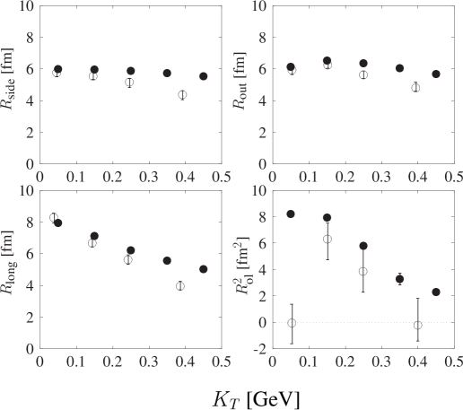
FIG. 1.: $K_{T}$ dependence of Cartesian HBT radii at the rapidity of $3\leq Y_{\pi\pi}\leq 4$. The reference frame is at $Y_{0}=3.5$. Open circles show the experimental results taken from NA49 preliminary data [23]. Closed circles show our results extracted from Eq. (32) through the Gaussian fitting.

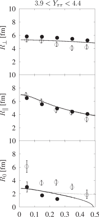
FIG. 2.: $K_{T}$ dependence of YKP radii. Being the same as in Fig. 1, open and closed circles show the experimental data and HBT radii, respectively. Solid lines stand for space-time extensions (49)-(51). Dotted lines stand for source sizes. ($\Delta z$ for $R_{\|}$ and $\Delta t$ for $R_{0}$.)

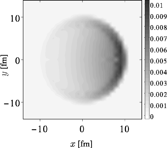
FIG. 3.: Source function $\bar{S}_{T}(x,y)$. Thick regions emit particles more than thin regions.

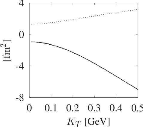
FIG. 4.: The second term $-2\langle\tilde{x}\tilde{t}\rangle/\beta_{\bot}$ (dotted line) and third term $((\Delta x)^{2}-(\Delta y)^{2})/\beta_{\bot}^{2}$ (solid line) in the right-hand side of Eq.(50) are functions of $K_{T}$. $Y_{\pi\pi}$ is fixed at 4.15.

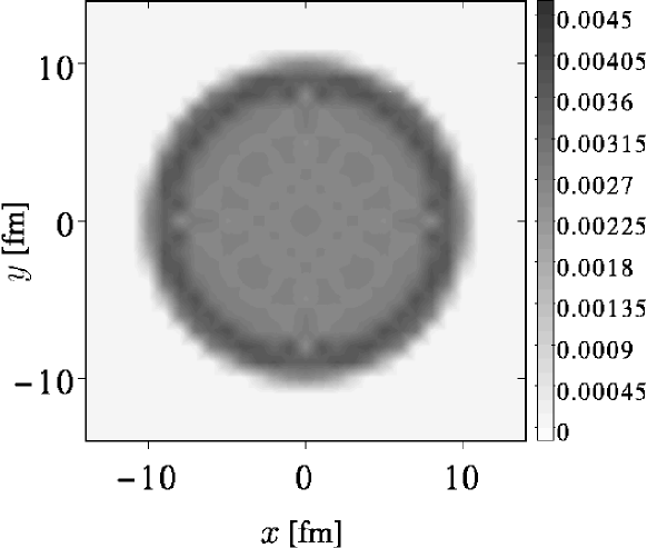
FIG. 5.: Same as Fig.3, but now the effect of transverse flow is neglected.

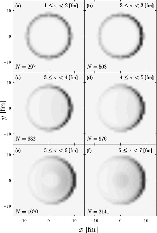
FIG. 6.: Source functions $S_{T}(x,y)$ sliced by freeze-out proper time. The thickness in each figure represents the intensity of the source.

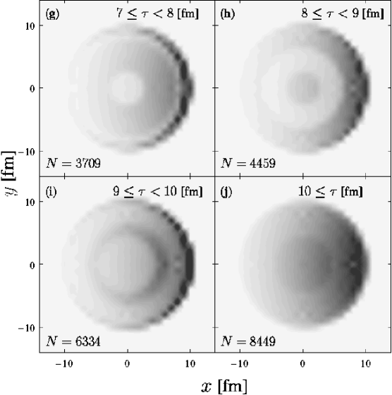
FIG. 7.: Rest of Fig. 6

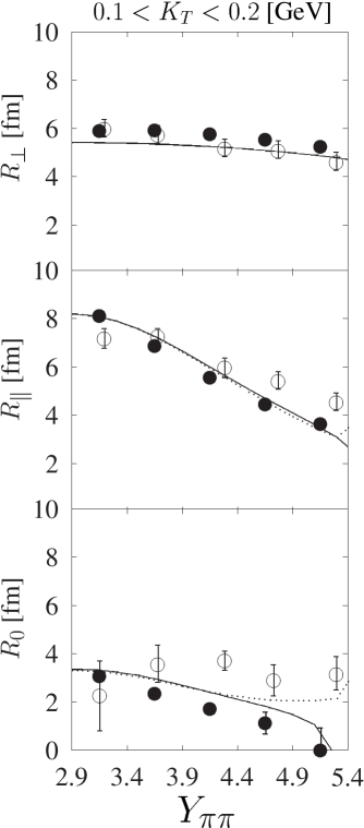
FIG. 8.: Pair rapidity $Y_{\pi\pi}$ dependence of YKP radii. As in Fig. 2, open circles, closed circles, solid lines and dotted lines stand for experimental results, our HBT radii, space-time extensions and source sizes, respectively.

FIG. 9.: Contour plot of source function for our model as a function of $\eta$ and $Y_{\pi\pi}$. The window of $Y_{\pi\pi}$ is adjusted to Fig. 8.

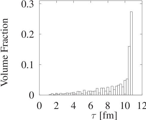
FIG. 10.: The volume fraction of freeze-out hypersurface as a function of $\tau$.

FIG. 11.: Contour plot of source function for the Gaussian source model (55) as a function of $\eta$ and $Y_{\pi\pi}$.

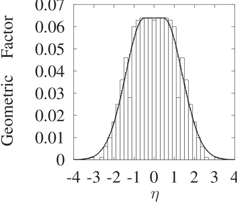
FIG. 12.: The geometric factor of source function in $\eta$–space. The box profiles stand for our hydrodynamical model. The solid line stands for modified geometric factor $\tilde{G}(\eta)$ obtained from the fit in Eq.(57) where $\eta_{0}=0.92$ and $\delta\eta=0.47$ .

FIG. 13.: Same as Fig. 11, but $G(\eta)$ is now replaced by $\tilde{G}(\eta)$ in the calculation.

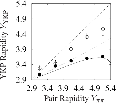
FIG. 14.: $Y_{\pi\pi}$ dependence of $Y_{YKP}$. Open circles stand for the experimental results. Closed circles stand for our result obtained through Eq. (58). The solid line stands for our result calculated from space-time extensions Eq.(44). The dotted line stands for average longitudinal expansion rapidity $\langle Y_{L}\rangle$ where $\langle\cdots\rangle$ is defined by Eq.(31). The dashed line stands for the infinite boost invariant source.

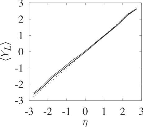
FIG. 15.: Average longitudinal rapidity versus longitudinal coordinate $\eta$. The thick line stands for $Y_{\pi\pi}=4.9$, and the thin line stands for $Y_{\pi\pi}=3.4$. The dotted line shows Bjorken’s scaling solution $Y_{L}=\eta$.

FIG. 16.: Rapidity distribution of primary negative charged hadrons ($\pi^{-},K^{-},\overline{p}$). Closed circles are taken from NA49 data [32]. The solid line stand for our numerical result.

FIG. 17.: Transverse mass distribution of negative charged hadrons ($\pi^{-},K^{-},\overline{p}$) successively scaled down by an order of magnitude in the rapidity range $y_{\pi}\in\{3.4,5.4\}$. Closed circles are taken from NA49 data [32]. The solid lines stands for our numerical results.

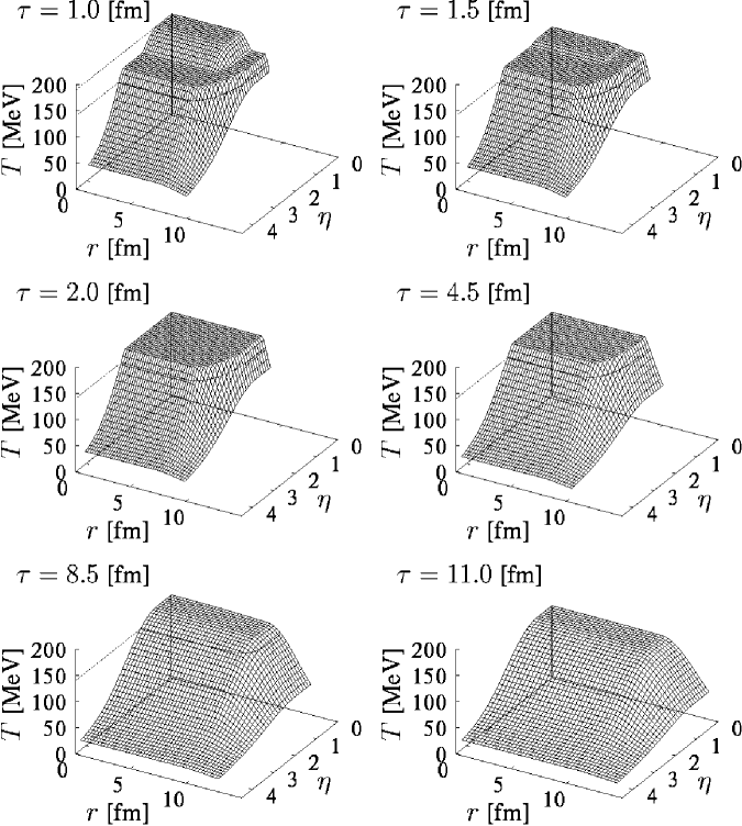
FIG. 18.: The space-time evolution of temperature-distribution with initial temperature (190 [MeV]), critical temperature (160 [MeV]) and freeze-out temperature (140 [MeV]). The flat area corresponds to the mixed phase region. From these graphs we can see that the QGP phase vanishes at $\tau$ = 2.0 [fm] and the mixed phase vanishes at $\tau$ = 8.5 [fm], and the temperature becomes less than the freeze-out temperature everywhere in the fluid at $\tau$ = 11.0 [fm].

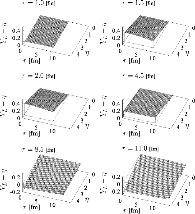
FIG. 19.: The space-time evolution of $Y_{L}-\eta$.

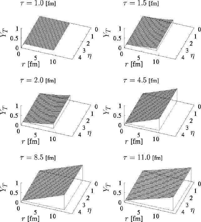
FIG. 20.: The space-time evolution of $Y_{T}$.

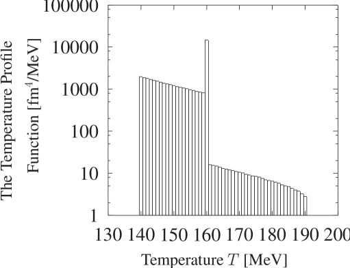
FIG. 21.: The temperature profile function.

REFERENCES

- [1] Quark Matter ’97, Proceedings of the Thirteenth International Conference on Ultra-Relativistic Nucleus–Nucleus Collisions, Tsukaba, Japan, December 1-5, 1997, edited by T. Hatsuda, Y. Miake, S. Nagamiya, and K. Yagi [Nucl. Phys. A638, 1c (1998)].
- [2] S. Pratt, Phys. Rev. D 33, 1314 (1986).
- [3] G. Bertsch and G. E. Brown, Phys. Rev. C 40, 1830 (1989).
- [4] R. Hanbury-Brown and R. Q. Twiss, Nature 178, 1046 (1956).
- [5] G. Goldhaber, T. Goldhaber, W. Lee, and A. Pais, Phys. Rev. 120, 300 (1960).
- [6] Y. Hama and S. S. Padula, Phys. Rev. D 37, 3237 (1988); A. N. Makhlin and Yu. M. Sinyukov, Z. Phys. C 39, 69 (1988).
- [7] B. R. Schlei, U. Ornik, M. Plümer, and R. M. Weiner, Phys. Lett. B293, 275 (1992).
- [8] S. Chapman, P. Scotto, and U. Heinz, Heavy Ion Physics 1, 1 (1995).
- [9] S. Chapman, P. Scotto, and U. Heinz, Phys. Rev. Lett. 74, 4400 (1995).
- [10] F. Yano and S. Koonin, Phys. Lett. B78, 556 (1978); M. I. Podgoretskiĭ, Sov. J. Nucl. Phys. 37, 272 (1983).
- [11] S. Chapman, J. R. Nix, and U. Heinz, Phys. Rev. C 52, 2654 (1995).
- [12] Y.-F. Wu, U. Heinz, B. Tomášik, and U. A. Wiedemann, Eur. Phys. J. C1, 599 (1998); U. Heinz, B. Tomášik, U. A. Wiedemann, and Y.-F. Wu, Phys. Lett. B382, 181 (1996).
- [13] S. Muroya and C. Nonaka, Bulletin of Tokuyama Women’s College, 6, 45 (1999); nucl-th/9709004.
- [14] H. Heiselberg and A. P. Vischer, Eur. Phys. J. C1, 593 (1998); Phys. Lett. B421, 18 (1998).
- [15] Y. Akase, M. Mizutani, S. Muroya, and M. Yasuda, Prog. Thoer. Phys. 85, 305 (1991); S. Muroya, H. Nakamura, and M. Namiki, Prog. Theor. Phys. Suppl. 120, 209 (1995).
- [16] J. Alam, S. Raha, and B. Sinha, Phys. Rep. 273, 243 (1996); J. Alam, D. K. Srivastava, B. Sinha, and D. N. Basu, Phys. Rev. D 48, 1117 (1993); K. Kajantie, M. Kataja, L. McLerran, and P. V. Ruuskanen, Phys. Rev. D 34,811 (1986).
- [17] S. Hioki, T. Kanki, and O. Miyamura, Phys. Lett. B261, 5 (1991); T. Hashimoto, K. Hirose, T. Kanki, and O. Miyamura, Z. Phys. C38, 251 (1988).
- [18] F. Cooper and G. Frye, Phys. Rev. D 10, 186 (1974).
- [19] Yu. M. Sinyukov, Z. Phys. 43, 401 (1989); H. Heiselberg, Heavy Ion Physics 5, 1 (1997).
- [20] F. Grassi, Y. Hama, and T. Kodama, Phys. Lett. B355, 9 (1995); M. I. Gorenstein and Yu. M. Sinyukov, Phys. Lett. B142, 425 (1984).
- [21] K. Morita, S. Muroya, and H. Nakamura, Prog. Theor. Phys. Suppl. 129, 185 (1997).
- [22] S. Pratt, T. Csörgő, and J. Zimányi, Phys. Rev. C 42, 2646 (1990).
- [23] K. Kadija et al., NA49 Collaboration, Nucl. Phys. A610, 248c (1996).
- [24] H. Appelshäuser et al., NA49 Collaboration, Eur. Phys. J. C2, 661 (1998).
- [25] B. R. Schlei and N. Xu, Phys. Rev. C 54, 2155 (1996).
- [26] B. R. Schlei, Phys. Rev. C 55, 954 (1997).
- [27] C. M. Hung and E. V. Shuryak, Phys. Rev. Lett. 75, 4003 (1995).
- [28] U. Heinz, Nucl. Phys. A638, 357c (1998).
- [29] B. Tomášik and U. Heinz, Report No. TPR-98-16, nucl-th/9805016 (1998).
- [30] I. G. Bearden et al. NA44 Collaboration, Phys. Rev. C 58, 1656 (1998).
- [31] J. D. Bjorken, Phys. Rev. D 27, 140 (1983).
- [32] S. V. Afanasiev et al. NA49 Collaboration, Nucl. Phys. A610, 188c (1996).
- [33] J. Sollfrank, P. Houvinen, M. Kataja, P. V. Ruuskanen, M. Prakash, and R. Venugopalan, Phys. Rev. C 55, 391 (1997).