Shell structure of superheavy nuclei in self-consistent mean-field models

Abstract

We study the extrapolation of nuclear shell structure to the region of superheavy nuclei in self-consistent mean-field models – the Skyrme-Hartree-Fock approach and the relativistic mean-field model – using a large number of parameterizations which give similar results for stable nuclei but differ in detail. Results obtained with the Folded-Yukawa potential which is widely used in macroscopic-macroscopic models are shown for comparison. We focus on differences in the isospin dependence of the spin-orbit interaction and the effective mass between the models and their influence on single-particle spectra. The predictive power of the mean-field models concerning single-particle spectra is discussed for the examples of ${}^{208}{\rm Pb}$ and the spin-orbit splittings of selected neutron and proton levels in ${}^{16}{\rm O}$, ${}^{132}{\rm Sn}$ and ${}^{208}{\rm Pb}$. While all relativistic models give a reasonable description of spin-orbit splittings, all Skyrme interactions show a wrong trend with mass number. The spin-orbit splitting of heavy nuclei might be overestimated by $40\%-80\%$, which exposes a fundamental deficiency of the current non-relativistic models. In most cases the occurrence of spherical shell closures is found to be nucleon-number dependent. Spherical doubly-magic superheavy nuclei are found at ${}^{298}_{184}114$, ${}^{292}_{172}120$, or ${}^{310}_{184}126$ depending on the parameterization. The $Z=114$ proton shell closure, which is related to a large spin-orbit splitting of proton $2f$ states, is predicted only by forces which by far overestimate the proton spin-orbit splitting in ${}^{208}{\rm Pb}$. The $Z=120$ and $N=172$ shell closures predicted by the relativistic models and some Skyrme interactions are found to be related to a central depression of the nuclear density distribution. This effect cannot appear in macroscopic-microscopic models or semi-classical approaches like the extended Thomas–Fermi-Strutinski integral approach which have a limited freedom for the density distribution only. In summary, our findings give a strong argument for ${}^{292}_{172}120$ to be the next spherical doubly-magic superheavy nucleus.

]

I Introduction

The extrapolation of nuclear shell structure to superheavy systems has been discussed since the early days of the shell correction method [1, 2, 3, 4, 5], when spherical proton shell closures at $Z=114$ and $Z=126$ and a spherical neutron shell closure at $N=184$ were predicted. Shell effects are crucial for the stability of superheavy nuclei which by definition have a negligible liquid-drop fission barrier. Recent experimental progress allowed the synthesis of three new superheavy elements with $Z=110$–$112$ [6, 7, 8, 9, 10], but these nuclides are believed to be well deformed. The experimental data on these nuclei and their decay products – $\alpha$-decay half-lives and $Q_{\alpha}$ values – agree with the theoretical prediction [11, 12, 13, 14, 15, 16] of a deformed neutron shell at $N=162$ which has a significant stabilizing effect [10, 17]. The experimental proof of the deformed shell by a measurement of the deformation is beyond the current experimental possibilities. As a first step in this direction the ground-state deformation of ${}^{254}{\rm No}_{102}$ was deduced from its ground-state rotational band in a recent experiment [18]. The ultimate goal is to reach the expected island of spherical doubly-magic superheavy nuclei. More refined parameterizations of macroscopic-microscopic models [13, 14, 15, 16] confirm the older finding that it is located around ${}^{298}_{184}114$. These nuclei, although even heavier than the heaviest nuclides known so far, are expected to have much longer half-lives due to the stabilizing effect of the spherical shell closure which significantly increases the fission barriers [19, 20, 21, 22].

Although modern macroscopic-microscopic models quite successfully describe the bulk properties of known nuclei throughout the chart of nuclei, their parameterization needs preconceived knowledge about the density distribution and the nuclear potentials which fades away when going to the limits of stability. Like the mean-field models based on the shell correction method, self-consistent mean-field models have been used for the investigation of superheavy nuclei from the earliest parameterizations [23, 24] to the most recent ones [25, 26, 27, 28, 29, 30, 31, 32, 33].

In two previous articles we have discussed the occurrence of spherical [31] and deformed [32] shell closures in superheavy nuclei for a large number of parameterizations of self-consistent nuclear structure models, namely the Skyrme-Hartree-Fock (SHF) approach [34], and the relativistic mean-field (RMF) model [35, 36, 37]. Spherical proton shell closures are predicted for $Z=114$, $Z=120$ and $Z=126$, depending on the parameterization, while neutron shell closures occur at $N=172$ and $N=184$ respectively. Only one parameterization – the Skyrme interaction SkI4 – confirms the prediction of macroscopic-microscopic models for a doubly magic ${}^{298}_{184}114$, other parameterizations – the Skyrme forces SkM* and SkP – predict ${}^{310}_{184}126$, while yet others – the Skyrme interaction SkI3 and most of the relativistic forces – give a new alternative with ${}^{292}_{172}120$. Several interactions predict no doubly magic spherical superheavy nucleus at all. In self-consistent models, the proton and neutron shells strongly affect each other [31]. Small details of the shell structure have a strong influence on the potential energy surfaces of superheavy nuclei in the vicinity of the ground-state deformation, leading to dramatic differences in the fission barrier heights and therefore in the fission half-lives, while the predictions of different models and forces are similar at large deformations [33].

Superheavy nuclei differ from stable nuclei by their larger charge and mass numbers. The strong Coulomb potential induces significant changes in the proton shell structure: single-particle states with large angular momentum and small overlap with the nuclear center only are lowered compared to small-$j$ states, see Figs. 1–2 of Ref. [30] and the discussion therein. While this effect occurs already in non-self-consistent models, polarization effects of the density distribution due to the high charge number can be described in self-consistent models only. The Coulomb interaction pushes protons to larger radii, which changes the density distribution and the single-particle potentials of both protons and neutrons in a complicated manner. On the other hand, the large mass number of superheavy nuclei leads to a high average density of single-particle levels. Therefore the search for shell effects in superheavy nuclei probes the detailed relations among the single-particle states with extremely high sensitivity.

The question arises which features of the effective mean-field models are most decisive for the single-particle structure. The three most crucial ingredients in this respect are: first the effective nucleon mass and its radial dependence which determines the level density near the Fermi surface, second the spin-orbit potential which determines the energetic distance of the spin-orbit partners, and third the density dependence of potential and effective mass which has an influence on the relative position of the states. We perform here a comparison of various parameterizations from SHF as well as RMF with emphasis on their spin-orbit properties. The effective masses (with one exception) are comparable in all forces. The density dependences are similar amongst the SHF forces and amongst the RMF forces, but differ significantly between SHF and RMF. The largest variations in the sample of parameterizations occurs indeed for the spin-orbit part of the forces where we have three classes, the standard SHF models, SHF with extended spin-orbit forces (SkI3 and SkI4), and the RMF models. The present paper concentrates predominantly on this given variation of the spin-orbit force. It is the aim of this paper to explain the contradicting results of self-consistent models mentioned above and to find the most reliable prediction for the next spherical doubly-magic superheavy nucleus.

In Sect. II the properties of the mean-field models and the parameterizations used is discussed. In Sect. III the details of the spin-orbit interaction and the differences between the various models used are explained, while Sect. IV discusses briefly the relation between effective mass and average density of single-particle levels. In Sect. V we compare the predictions of the various mean-field models with known single-particle energies in ${}^{208}{\rm Pb}$ and experimental spin-orbit splittings in ${}^{16}{\rm O}$, ${}^{132}{\rm Sn}$ and ${}^{208}{\rm Pb}$ and study the shell structure of the potential spherical doubly-magic nuclei ${}^{298}_{184}114$, ${}^{292}_{172}120$, and ${}^{310}_{184}126$ and the predicted nucleon-number dependence of the $Z=120$ proton shell and the $N=172$ neutron shell in some detail. Sect. VI summarizes our findings. In an appendix we present the details of the mean-field and pairing models necessary for our discussion.

II The framework

The Skyrme force was originally designed as an effective two-body interaction for self-consistent nuclear structure calculations. It has the technical advantage that the exchange terms in the Hartree-Fock equations have the same form as the direct terms and therefore the numerical solution of the Skyrme-Hartree-Fock equations is as simple as in case of the Hartree approach, while the solution of the Hartree-Fock equations using finite-range forces like the Gogny force [38] is a numerically challenging task. The total binding energy can be formulated in terms of an energy functional which depends on local densities and currents only, see Appendix A. This links the Skyrme-Hartree-Fock model to the effective energy functional theory in the Kohn-Sham approach which was originally developed for many-electron systems. The Hohenberg-Kohn theorem [39] states that the non-degenerate ground-state energy of a many-Fermion system with local two-body interactions is a unique functional of the local density only. The Kohn-Sham scheme [40] relies on the Hohenberg-Kohn theorem but keeps the full dependence on the single-particle wavefunctions for the kinetic energy which allows to preserve the full shell structure while employing for the rest rather simple functionals in local-density approximation. This point of view can be carried over to the case of nuclei where, however, the non-local two-body interaction requires an extension of the energy functional by a dependence on other densities and currents, e.g., the spin-orbit current. In any case, there is no need for a fundamental two-body force in an effective many-body theory, but one can start from an effective energy functional which is formulated directly at the level of one-body densities and currents (see, e.g., [41] and references therein).

The relativistic mean-field model can be seen from the same point of view as a relativistic generalization of the non-relativistic models using a finite-range interaction formulated in terms of effective mesonic fields. Relativistic kinematics plays no role in nuclear structure physics, but the RMF naturally describes the spin-orbit interaction in nuclei, which is a relativistic effect that has to be added phenomenologically in non-relativistic models. This will be discussed in Sect. III in more detail.

For both SHF and RMF there are numerous parameterizations in the literature. We select here a few typical samples of comparable (high) quality, mostly from recent fits. For the non-relativistic Skyrme-Hartree-Fock calculations we consider the Skyrme forces SkM* [42], SkP [43], SLy6, SLy7 [44, 45], SkI1, SkI3, and SkI4 [46]. For the RMF we consider NL3 [47], NL-Z, [48], and two completely new forces, NL-Z2 and NL-VT1. All forces are developed through fits to given nuclear data, but with different bias. Of course, the basic ground-state properties of spherical nuclei (energy, radius) are always well reproduced. Small variations appear with respect to further demands. The parameterization ${\rm SkM}^{\ast}$ is the oldest in the list here. It was the first Skyrme force with acceptable incompressibility as well as fission properties and remains up to date a reliable parameterization in several respects. The Skyrme force SkP was developed around the same time with the aim to allow the simultaneous description of mean-field and pairing channel. Moreover, it was decided here to use effective mass $m^{\ast}/m=1.0$. (Mind that all other forces in our sample have smaller effective masses around $0.6\leq m^{\ast}/m\leq 0.8$). The forces SLy6 and SLy7 stem from a series of fits where it was successfully attempted to cover properties of neutron matter together with normal nuclear ground-state properties. In SLy6 the contribution of the kinetic terms of the Skyrme force to the spin-orbit potential is discarded, which is common practice for nearly all Skyrme parameterizations, e.g. SkM* and the SkI$x$ forces in the sample here. SLy7 is fitted exactly in the same way as SLy6, but these additional contributions to the spin-orbit force are considered, see the discussion in Sect. III A for details. The forces SkI1, SkI3 and SkI4 stem from a recent series of fits along the strategy of [49] where additionally key features of the nuclear charge formfactor were included providing information on the nuclear surface thickness. For these, furthermore, information from exotic nuclei was taken into account in order to better determine the isotopic parameters. The force SkI1 is a fit within the standard parameterization of the Skyrme forces. This performs very well in all respects, except for the isotopic trends of the charge radii in the lead region. To cover these data, one needs to extend the spin-orbit functional by complementing it with an additional isovector degree of freedom [46] as will be discussed in Sect. III A in more detail. SkI3 uses a fixed isovector part built in analogy to the RMF, whereas SkI4 was fitted allowing free variation of the isovector spin-orbit force. The modified spin-orbit force has a strong effect on the spectral distribution in heavy nuclei and thus even more influence for the predictions of shell closures in the region of superheavy nuclei.

The forces headed by “NL” belong to the domain of the RMF model. The parameterizations NL-Z, NL-Z2, and NL3 use the standard nonlinear ansatz for the RMF model, whereas NL-VT1 additionally considers a tensor coupling of the vector mesons. The parameterization NL-Z [36] aims at a best fit to nuclear ground-state properties along the strategy of [49]. It is a re-fit of the popular force NL1 with a microscopic treatment of the correction for spurious center-of-mass motion. NL-Z2 and NL-VT1 are new parameterizations developed for the purpose of these studies to match exactly the same enlarged set of data including information on exotic nuclei like the SkI$x$ Skyrme forces. This should allow better comparison between the RMF and the Skyrme model. The force NL3, finally, results from a recent fit including neutron rms radii. It gives a good description of both nuclear ground states and giant resonances. Details of the RMF Lagrangian and the actual parameterizations are discussed in Appendix A 2.

TABLE I.: Compilation of nuclear matter properties for the parameter sets used in this study. $E/A$ and $\rho_{0}$ denote the equilibrium energy per nucleon and density, $K_{\infty}$ the compression modulus, $m^{\ast}/m$ the effective mass in units of the free mass (note that we provide two values for the relativistic models where the value in brackets is $m^{\ast}/m(k_{F})$ at the Fermi surface and the other at $k\!=\!0$ [64]) $a_{\rm sym}$ the asymmetry coefficient, and $\kappa$ the sum–rule enhancement factor.

Force	$E/A\,[{\rm MeV}]$	$\rho_{0}\,[{\rm fm}^{-3}]$	$K_{\infty}\,[{\rm MeV}]$	$m^{\ast}/m$	$a_{\rm sym}$	$\kappa$
SkP	$-16.04$	$0.163$	$202$	1.000	$30.0$	0.35
SkM∗	$-16.01$	$0.160$	$217$	0.789	$30.0$	0.53
SLy6	$-15.92$	$0.159$	$230$	0.690	$32.0$	0.25
SLy7	$-15.90$	$0.158$	$230$	0.688	$32.0$	0.25
SkI1	$-15.93$	$0.160$	$243$	0.693	$37.5$	0.25
SkI3	$-15.96$	$0.158$	$258$	0.577	$34.8$	0.25
SkI4	$-15.92$	$0.160$	$248$	0.650	$29.5$	0.25
NL3	$-16.24$	$0.148$	$272$	0.595 (0.659)	$37.4$	0.68 (0.53)
NL–Z	$-16.18$	$0.151$	$173$	0.583 (0.648)	$41.7$	0.72 (0.55)
NL–Z2	$-16.07$	$0.151$	$172$	0.583 (0.648)	$39.0$	0.72 (0.55)
NL–VT1	$-16.10$	$0.150$	$179$	0.600 (0.663)	$39.0$	0.66 (0.51)

The nuclear matter properties of the forces are summarized in Table I. These are to be considered mainly as extrapolations from finite nuclei to the infinite system. There a few exceptions because in some cases the one or the other nuclear matter property has entered as a constraint into the fit. These cases are: the effective mass $m^{\ast}/m=1$ for SkP, the compressibility $K_{\infty}=230\;{\rm MeV}$ and asymmetry coefficient $a_{\rm sym}=32.0\;{\rm MeV}$ for the SLy$x$ forces, and the sum-rule enhancement factor $\kappa=0.25$ in case of the SLy$x$ and SkI$x$ forces. Table I shows that most Skyrme forces share the basic nuclear matter properties close to the phenomenological values like binding energy per nucleon $E/A\approx-16\;{\rm MeV}$, equilibrium density $\rho_{0}\approx 0.16\;{\rm fm}^{-3}$, incompressibility $K=210\pm 30\,{\rm MeV}$ [50], asymmetry energy $30\,{\rm MeV}\leq a_{\rm sym}\leq 32\,{\rm MeV}$, and a low sum-rule enhancement factor $0\leq\kappa\leq 0.25$. A phenomenological value for the effective mass of $m^{*}/m\approx 0.8$ can be drawn from the position of the giant quadrupole resonance in heavy nuclei [51]. And we see that the mean field results for the effective mass vary in a wide range $0.58\leq m^{\ast}/m\leq 1.0$ about this value. This is a bit disquieting because the effective mass is a feature which has a strong impact on spectral properties, influencing, in turn, the predictions for superheavy nuclei.

The nuclear matter properties of the relativistic parameterizations differ significantly from those of Skyrme forces. $E/A$ is usually slightly larger and $\rho_{0}$ somewhat smaller than the values for Skyrme interactions. The predictions for the incompressibility $K$ differ systematically from those of the nonrelativistic models, in case of NL3 it is somewhat larger, in case of the other RMF forces smaller than the average result for Skyrme forces. But all parametrizations stay within the accepted bounds of this rather uncertain quantity. The asymmetry coefficient and the sum-rule enhancement factor are substantially larger than in case of the Skyrme forces. But all RMF forces agree in their rather low value for the effective mass $0.58\leq m^{\ast}/m\leq 0.6$. It is to be noted, however, that the effective mass in RMF depends on the momentum as

$$\frac{m^{*}(k_{F})}{m} = \sqrt{\left(\frac{m^{*}(0)}{m}\right)^{2}+\left(\frac{k_{F}}{m}\right)^{2}}$$ (1)

$$\approx \sqrt{\left(\frac{m^{*}(0)}{m}\right)^{2}+0.08}$$ (2)

where $m^{*}(0)$ is the value at $k=0$ usually handled as effective mass in the RMF and where we assumed in the second step a typical $k_{F}\approx 1.35/{\rm fm}$. Table I thus shows two values for $m^{*}/m$ in case of the RMF, at momentum zero and in brackets the more relevant value $m^{*}/m(k_{F})$ at the Fermi surface. The latter value is larger by about $10\%$ and comes visibly closer to the results for the Skyrme forces.

In view of the application to superheavy nuclei, it is worthwhile to check the performance of all these forces in our sample with respect to already known superheavy nuclei. This was done in Ref. [32]. It turns out, that SkI3, SkI4, and the relativistic forces perform best in that respect, although it is to be mentioned that all relativistic forces show a wrong isotopic trend, see [32] for details. It is noteworthy that the extended Skyrme functionals SkI3 and SkI4 perform much better in the region of superheavy nuclei than the Skyrme parameterizations with the standard spin-orbit interaction. This indicates that an extended spin-orbit interaction is an essential ingredient for the description of heavy systems.

In both SHF and RMF the pairing correlations are treated in the BCS scheme using a delta pairing force, see Appendix A 3 for details.

The numerical procedure solves the coupled SHF and RMF equations on a grid in coordinate space with the damped gradient iteration method [52]. The codes for the solution of both SHF and RMF models have been implemented in a common programming environment sharing all the crucial basic routines.

III Spin-orbit interaction in nuclear mean-field models

A The spin-orbit field

The spin-orbit interaction is an essential ingredient of every model dealing with nuclear shell structure to explain the shell closures of heavy nuclei beyond $N=Z=20$ [53, 54]. It was already noted in the first explorations with the modified oscillator model that different fits of the spin-orbit coupling constant lead to contradicting predictions for the next major shell closures in superheavy nuclei [55].

The spin-orbit interaction emerges naturally in relativistic models and the explanation of the large spin-orbit splitting in nuclei was one of the first prominent successes of the relativistic mean-field approach [56]. The spin-orbit potential can be deduced in the non-relativistic limit of the RMF and is given up to order $v^{2}/c^{2}$ by [36]

$${\bf W}_{q}^{({\rm rmf})}\approx-\frac{\hbar c}{(2m_{q}+{\cal S}_{q}-{\cal V}_{q})^{2}}\nabla({\cal S}_{q}-{\cal V}_{q})\quad,$$ (3)

where ${\cal S}$ and ${\cal V}$ are the scalar and vector potentials respectively, see appendix A 2 for details. While the usual potential is given by the sum of the large negative scalar potential ${\cal S}$ and the large positive vector potential ${\cal V}$ which cancel nearly to give the usual shell-model potential, the difference of scalar and vector potential enters the expression for the spin-orbit field, explaining its large strength. The occurrence of the derivative of the fields in (3) indicates that the spin-orbit field is peaked in the nuclear surface region and that its strength will depend on the surface thickness of the particular nucleus.

To compare with the corresponding expression for Skyrme interactions, one has to evaluate (3) in local density approximation

$${\bf W}_{q}^{{(\rm rmf})}\approx\frac{\hbar c}{(2m_{q}-C\rho-C^{\prime}\rho_{q})^{2}}\;(C\nabla\rho+C^{\prime}\nabla\rho_{q})\quad,$$ (4)

where $C=C_{\sigma}+C_{\omega}-C_{\rho}$ and $C^{\prime}=2C_{\rho}$ are combinations of RMF parameters with $C_{i}=g_{i}^{2}/m_{i}^{2}$. The isospin dependency of the spin-orbit potential is rather weak for typical RMF parameterizations which give $C^{\prime}\approx 0.1\times C$.

In the framework of non-relativistic models the zero-range two-body spin-orbit interaction proposed by Bell and Skyrme [57, 58] is widely used. Examples are all standard Skyrme interactions like SkM*, SkP, the SLy$x$ forces or SkI1 and other non-relativistic effective interactions like the Gogny force [38]. The corresponding spin-orbit potential ${\bf W}_{q}$ is given by

$${\bf W}_{q}^{{(\rm std})}=b_{4}(\nabla\rho+\nabla\rho_{q})\quad.$$ (5)

There are two fundamental differences between the relativistic and non-relativistic expressions for the spin-orbit potential: the isospin dependence and the missing density dependence in case of the non-relativistic models.

When deriving the single-particle Hamiltonian from an underlying Skyrme force there appears an additional contribution to the spin-orbit field which arises from the momentum-dependent terms in the two-body Skyrme force

$${\bf W}_{q}^{({\bf J})}=b_{4}(\nabla\rho+\nabla\rho_{q})+c_{1}{\bf J}-c_{1}^{\prime}{\bf J}_{q}\quad.$$ (6)

The calculation of the spin-orbit current ${\bf J}$ is somewhat cumbersome in deformed codes and its contribution to the total binding energy rather small. Therefore the ${\bf J}$-dependent terms in (6) are discarded in most parameterizations of the Skyrme interaction and (5) is used instead. SkP and SLy7 are two exceptions in this investigation.

In the Hohenberg-Kohn-Sham interpretation of the Skyrme interaction outlined above, there is no need for an underlying two-body force, but one can start from an effective energy functional which is formulated directly at the level of local one-body densities and currents. This relaxes the fixed isotopic mix (5) in the spin-orbit functional and allows more freedom for its parameterization which was used to complement the spin-orbit interaction by an explicit isovector degree of freedom in the fit of the extended Skyrme functionals SkI3 and SkI4

$${\bf W}_{q}^{({\rm ext})}=b_{4}\;\nabla\rho+b_{4}^{\prime}\;\nabla\rho_{q}\quad.$$ (7)

The additional isospin degree-of-freedom enables the reproduction of the kink in the isotope shifts of charge mean-square radii in lead, which is not possible with standard Skyrme forces employing (5) [46, 59, 60], while the experimental data are reproduced by most RMF forces. The parameters $b_{4}$ and $b_{4}^{\prime}$ in SkI3 and SkI4 are adjusted to reproduce the spin-orbit splittings of protons and neutrons in ${}^{16}{\rm O}$ and the isotope shifts of charge mean-square radii in lead. As a result of the fit the approximate relation $b_{4}\approx-b_{4}^{\prime}$ emerges for SkI4, see also Table II in Appendix A 1. This means that for SkI4 the spin-orbit potential of one kind of nucleons depends mainly on the density profile of the other kind of nucleons. The force SkI3 was adjusted with the same fit strategy but with a fixed isovector part $b_{4}^{\prime}=0$ analogous to the RMF in the sense that the spin-orbit potentials of protons and neutrons are approximately equal. However, there remain differences between SkI3 and the RMF: all RMF potentials have a finite range and the spin-orbit interaction has a small but non–zero isospin dependence and a strong density dependence.

B Spin–orbit splitting

In non-relativistic models the spin-orbit term in the equation-of-motion of the radial wavefunctions in case of spherical symmetry is given by

$$W_{q,r}{\textstyle\frac{1}{r}}\big{[}j_{k}(j_{k}+1)-\ell_{k}(\ell_{k}+1)-{\textstyle\frac{3}{4}}\big{]}\;\phi_{k}(r)\quad,$$ (8)

where $W_{q,r}$ is the radial component of the spin-orbit potential and $\phi(r)$ the radial part of the single-particle wavefunction $\psi({\bf r})$. For well-bound single-particle states, the radial wavefunctions $\phi_{\ell\pm 1/2}$ entering Eq. (8) are only slightly different. Therefore the contributions from the potential and the kinetic term can be neglected in very good approximation when calculating the spin-orbit splitting $\Delta\epsilon_{\rm LS}=\epsilon_{\ell+1/2}-\epsilon_{\ell-1/2}$ of two states $\phi_{j}$ with the same radial quantum number and orbital angular momentum $\ell$ but different $j=\ell\pm 1/2$

$$\Delta\epsilon_{\rm LS} \approx 4\pi\int\limits_{0}^{\infty}\!{\rm d}r\,r\,W_{q,r}\big{(}\ell+{\textstyle\frac{1}{2}}\big{)}\Big{[}\big{(}\ell+{\textstyle\frac{3}{2}}\big{)}|\phi_{\ell+1/2}|^{2}$$ (10)

$$\quad-\big{(}\ell+{\textstyle\frac{1}{2}}\big{)}|\phi_{\ell-1/2}|^{2}\Big{]}\quad.$$

The spin-orbit splitting scales with $2\ell+1$ and depends sensitively on the overlap of the single-particle wavefunctions with $W_{q,r}/r$. The shape of $W_{q,r}/r$ – which is usually peaked at the nuclear surface – depends itself on the variation of the actual density distribution in the nucleus which changes going along isotopic or isotonic chains, especially when the density distribution becomes diffuse going towards the drip-lines or when it develops a central depression – as happens in some superheavy nuclei, see Sect. V D.

Equation (10) holds as well for the non-self-consistent single-particle models which are used in the framework of macroscopic-microscopic models. There the spin-orbit potential ${\bf W}$ is assumed to be proportional to the gradient of the single-particle potential $U$. In the simplest case of the modified oscillator model – which was used in the first studies of the shell structure of superheavy nuclei [2, 3] – the spin-orbit potential $W/r$ has no radial dependence, the amplitude of the spin-orbit splitting is simply proportional to $2\ell+1$, see [55] for a detailed discussion. In more refined single-particle models like the Folded-Yukawa model (FY) [61] or Woods-Saxon model [62] the spin-orbit potential is peaked at the nuclear surface like in the self-consistent models, see appendix A 4 for details.

IV Effective mass and average level density

The average density of single-particle levels $g(\epsilon)$ in the vicinity of the Fermi energy can be estimated using the Fermi gas model in a finite potential well. In case of non-relativistic particles one obtains [63]

$$g_{q}^{\rm SHF}(\epsilon_{\rm F,q})\approx\frac{3}{4}\;N_{q}\;\frac{2m^{\ast}_{q}}{(\hbar k_{\rm F,q})^{2}}\quad,$$ (11)

The relativistic generalization of formula (11) is simply obtained by inserting the effective mass $m^{\ast}(k_{F})$ at the Fermi surface, see eq. (1) and the values in brackets in table I).

The average level density rises linearly with particle number – the single-particle spectra of superheavy nuclei are therefore much denser than those of lighter stable nuclei. This makes the shell structure of superheavy nuclei very sensitive to details of the spin-orbit interaction, differences of a few $100\;{\rm keV}$ in the spin-orbit splitting of two given orbitals can create or destroy shell closures.

The level density depends linearly on the effective mass $m^{\ast}$ as well. This causes a dramatic difference when comparing the predictions of interactions with small effective mass, e.g. SkI3 with $m^{\ast}/m=0.574$, and parameterizations with large effective mass like SkP with $m^{\ast}/m=1.0$ in the region of superheavy nuclei. As said before, a phenomenological value of $m^{\ast}/m\approx 0.8$ for the isoscalar effective mass can be determined from the position of the isoscalar quadrupole giant resonances which is just in between the extremes spanned by our choice of mean field models. But a word of caution is in place here. The value of $0.8$ is appropriate for the effective mass in the nuclear volume. But the value may be larger at the surface, or Fermi surface respectively [64]. This is, admittedly, a feature which is not yet built into nowadays mean field models. A thorough exploration of this aspect is a task for future reasearch.

V Spherical magic numbers

A Relation of single-particle spectra and bulk properties

At closed shells, one observes a sudden jump in the two-nucleon separation energies $S_{2q}$

$$S_{2q}(N_{q})=E(N_{q}-2)-E(N_{q})\quad.$$ (12)

$N_{q}$ and the number of the other kind of nucleons are assumed to be even. The two-nucleon separation energy is a better tool to quantify shell effects than the single-nucleon separation energy due to the absence of odd-even effects. It is a very good approximation for twice the negative Fermi energy

$$S_{2q}(N,Z)\approx-2\lambda_{q}(N,Z)\quad.$$ (13)

In doubly-magic nuclei – in which the BCS pairing model breaks down – the Fermi energy is simply given by the single-particle energy of the last occupied state. Deviations between the calculated and experimental values for the single-particle energy of the last occupied state in doubly magic nuclei are therefore connected by (13) with an error in the two-nucleon separation energies below the shell closure. Although slightly influenced by pairing correlations, this holds in good approximation also for the first unoccupied state above the Fermi surface and the two-nucleon separation beyond the shell closure.

The size of the gap in the single-particle spectrum is given by half the difference in Fermi energy when going from a closed shell nucleus to a nucleus with two additional like nucleons. But from Eq. (13) it follows that this is in very good approximation equal to the shell gap $\delta_{2q}$, the second difference of the binding energy

$$\delta_{2q}(N_{q}) = E(N_{q}+2)-2E(N_{q})+E(N_{q}-2)$$ (14)

$$\approx -2[\lambda_{q}(N_{q}+2)-\lambda_{q}(N_{q})]\quad,$$ (15)

which was used in [31] to quantify the magicity of a nucleus. Going away from closed shells, there is a non-negligible contribution from the residual pairing interaction, therefore $S_{2q}$ and $\delta_{2q}$ loose their direct relation to the single-particle levels. The two-nucleon gaps $\delta_{2q}$ represent the size of the gap in the single-particle spectra, but they do not contain information about the actual location of the single-particle energies.

Only interactions which reproduce the experimental values of the first single-particle state below and above the Fermi surface will give the correct binding energies around closed shell nuclei. This can be read the other way round as well: Only interactions which reproduce the binding energies around shell closures give a good description of at least the first single-particle state below and above the shell closure, but the bulk properties give no information on single-particle states away from the Fermi energy. This demonstrates nicely, however, that total binding energy and properties of single-particle states are connected in self-consistent mean-field models. This is very different in macroscopic-microscopic models where the bulk properties and single-particle spectra are described in separate models.

One has to be careful when comparing experimental and calculated single-particle spectra. Experimental single-particle energies of even-even nuclei are deduced from excitation energy measurements of adjacent odd-mass nuclei. The binding energy of odd-mass nuclei is affected by polarization effects induced by the odd nucleon, see [65] for a discussion of these effects in the framework of the RMF. The polarization effects are important for the comparison of calculated and experimental single-particle energies. But they do not affect the relation between the single-particle spectra and the bulk properties in even-even nuclei discussed here.

B The single-particle spectra in known nuclei

Before extrapolating the models to the regime of superheavy nuclei we want to test the predictive power of the mean-field models looking at ${}^{208}{\rm Pb}$, the heaviest known spherical doubly-magic nucleus. Figure 1 shows the single-particle spectra of ${}^{208}{\rm Pb}$ as obtained from spherical calculations with the mean-field forces as indicated. The upper panel shows the spectrum of the protons, the lower panel that of the neutrons. The experimental excitation energies in the neighboring odd nuclei are shown on the left side for comparison, the data are taken from [66]. The gaps in the single-particle spectra at $Z=82$ and $N=126$ are clearly visible, but the forces obviously do not agree for this stable nucleus, which was used in the fit of all parameter sets employed here.

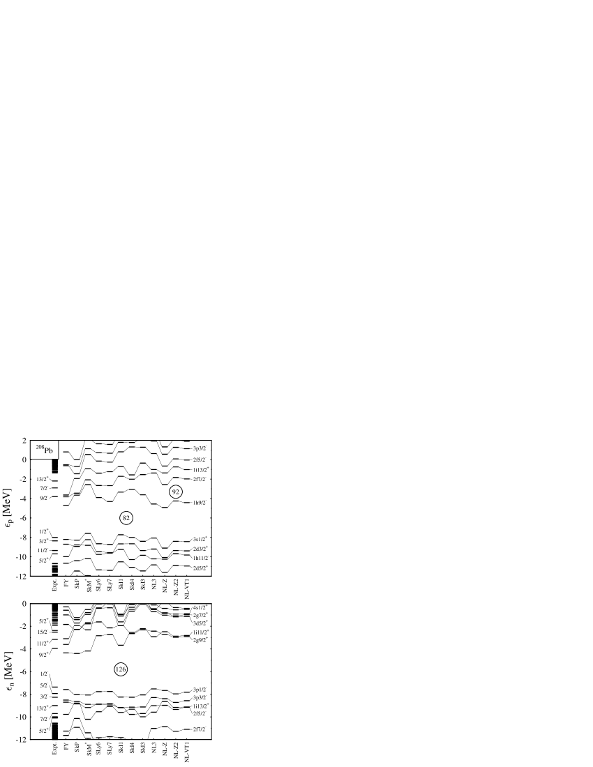
FIG. 1.: Single–particle spectrum of the protons (upper panel) and neutrons (lower panel) in ${}^{208}{\rm Pb}$ calculated with the mean–field forces as indicated.

As already discussed in Sect. V A, the difference between the calculated and experimental energies of the first single-particle state above and below the shell closure reflects the quality of the description of the total binding energies in the vicinity of a shell closure. There are large differences between the forces in their predictions for states further away from the Fermi surface. The spectrum predicted by SkP is much too dense and the ordering of proton states below the Fermi surface not reproduced. A natural explanation for this might the too large effective mass of SkP, but one has to be careful: The effective mass determines the average level density only but not the level density in an actual nucleus. The difference in energies between the $2g_{9/2^{+}}$ and $1i_{11/2^{+}}$ neutron states is, for example, by far too large when calculated with SkP and SkM^∗, leading to a sub-shell closure at $N=136$ in contradiction to experimental data. In the RMF and extended Skyrme forces this difference is by far too small, NL3 predicts even a wrong ordering of these two levels. The relativistic forces and the relativistic corrected Skyrme force SkI3 overestimate the gap between the proton $1h_{9/2^{-}}$ and $2f_{7/2^{-}}$ states above the Fermi surface which leads to a pronounced sub-shell closure at $Z=92$ which again is in contradiction with experiment.

The RMF models and the modern Skyrme forces with small effective mass push the $1j_{15/2^{-}}$ with an experimental single-particle energy of $\epsilon=-2.51\;{\rm MeV}$ too much up in the spectrum, e.g. to $\epsilon=-0.418\;{\rm MeV}$ in NL-VT1, while Skyrme forces with a large effective mass like SkM^∗ and SkP work slightly better within this respect. The differences in average level density due to the actual value of the effective mass scale only the deviation from the experimental value. States with large orbital angular momentum systematically lie too high in the single-particle spectrum for all forces, see also the proton $1i_{13/2^{+}}$ state. As this problem appears for all parameterizations of both SHF and RMF models and for all nuclei throughout the chart of nuclei [67, 68], we conclude that this is not a problem of actual fits but it indicates the need for improved effective interactions beyond the current energy functionals.

All forces have problems to reproduce the neutron single-particle energies below the Fermi energy as well. All relativistic forces and SkI3 give a wrong level ordering, the $2f_{5/2^{-}}$ state lies too low in energy in all cases. Standard Skyrme forces work slightly better in that respect, e.g. SkP predicts $2f_{5/2^{-}}$ to be the second-to-last state below the Fermi surface, but interchanges the $3p_{3/2^{-}}$ and $1i_{13/2^{+}}$ states instead, the latter one is again pushed up too much in energy like all other states with large angular momentum. It is remarkable that the non-self-consistent FY model is the only one which reproduces the level ordering of all states in the vicinity of the Fermi energy for both protons and neutrons. Like the self-consistent models, however, it is not able to reproduce the values of the single-particle energies or even their relative distance.

To conclude our findings so far: the comparison between predictions of various current mean-field models and experimental data shows that the models are not able to reproduce all details of experimental single-particle spectra and show additionally significant differences among each other which are related to effective mass and details of the spin-orbit interaction.

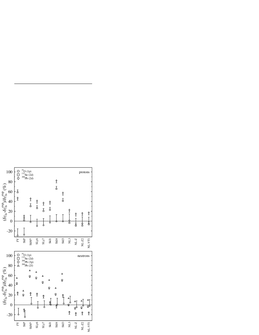
FIG. 2.: Relative error $(\delta\epsilon_{ls}-\delta\epsilon_{ls}^{\rm expt})/\delta\epsilon_{ls}^{\rm expt}$ in percent of the spin–orbit splitting of proton (upper panel) and neutron (lower panel) single–particle states close to the Fermi surface in ${}^{16}{\rm O}$, ${}^{132}{\rm Sn}$, and ${}^{208}{\rm Pb}$ calculated from the mere mean–field single–particle energies with the parameterizations as indicated.

Shell closures of heavy nuclei are related to the spin-orbit splitting of states with large orbital angular momentum. Therefore it is interesting to compare the predictions of the mean-field models with experimental data on spin-orbit splittings in known nuclei. Figure 2 shows the relative errors in $\%$ of the spin-orbit splittings of neutron levels (lower panel) and proton levels (upper panel) near the Fermi surface in ${}^{16}{\rm O}$, ${}^{132}{\rm Sn}$ and ${}^{208}{\rm Pb}$. Negative errors denote theoretical values which are too small. The spin-orbit splittings are calculated from the single-particle energies as they come out from a spherical mean-field calculation. As already mentioned, the experimental single-particle energies are measured as separation energies between adjacent nuclei, where polarization effects have a visible influence. The error bars in Fig. 2 represent the uncertainty of the spin-orbit splittings due to polarization effects as they are found in [65].

All RMF forces reproduce the experimental spin-orbit splittings fairly well, although there are deviations up to $20\%$ which are scattered around zero. The errors from all RMF forces are similar and therefore it is likely that these errors represent the standard RMF Lagrangian, not specific parameterizations. Although the tensor couplings of the vector mesons in NL-VT1 change the relative distance of the single-particle energies compared to NL-Z2, see Fig. 1, they have no visible influence on the spin-orbit splittings compared to the standard Lagrangian. It is interesting that the errors of the spin-orbit splittings of the neutron $3p$ and $2f$ states in ${}^{208}{\rm Pb}$ have the largest values but different sign while ${}^{16}{\rm O}$ and ${}^{132}{\rm Sn}$ are described very well. There is only one splitting known for protons in ${}^{208}{\rm Pb}$ (if one excludes splittings across the Fermi surface which have a large theoretical uncertainty, see [65]), so one has no information how the error depends on the angular momentum of the state as in the case of neutrons. But, however, the RMF gives a very good overall description of spin-orbit splittings throughout the chart of nuclei without any free parameters adjusted to single-particle data.

The reproduction of the experimental data with the Skyrme functionals is by far not as good as for the relativistic models. There is a clear trend which is the same for all standard Skyrme forces: for neutrons the error of the $1p$ splitting in ${}^{16}{\rm O}$ has the smallest value, then comes the splitting of the $3p$ state in ${}^{208}{\rm Pb}$, the $2d$ state in ${}^{132}{\rm Sn}$ and then the splitting of the $2f$ state in ${}^{208}{\rm Pb}$. Like in the case of the RMF, the splittings of the $2f$ and $3p$ neutron states in ${}^{208}{\rm Pb}$ are not reproduced with the same quality, the error for the $2f$ state is always much larger compared to the experimental value than for the $3p$ state.

FIG. 3.: Two–proton gap in the chain of $Z=114$ isotones calculated with the forces as indicated.

It is very unlucky that the parameters of the spin-orbit interaction in non-relativistic models are usually adjusted to data in ${}^{16}{\rm O}$, which is at the lower end of a systematic trend increasing with mass number. Choosing one or several heavier nucleus for the fit, however, does not cure the problem of the wrong trend, but it gives a better overall description of spin-orbit splittings as can be seen from SkP, which gives the best possible compromise for a standard Skyrme force: the differences between the data points are similar to those from the other standard Skyrme forces, but they are centered around zero. The other standard Skyrme forces, SkM^∗, SLy6, SLy7, and SkI1, give similar predictions, with large errors for the $2d$ states in ${}^{132}{\rm Sn}$ and the neutron $2f$ and proton $2d$ state in ${}^{208}{\rm Pb}$.

The predictions of the extended Skyrme forces SkI3 and SkI4 deviate significantly from both the standard Skyrme forces and the RMF. SkI3 gives bad results for neutrons and protons and shows surprising large differences to the relativistic forces. This is somewhat unexpected because SkI3 was constructed with the isospin dependence of the spin-orbit force which appears in the relativistic models. This indicates that the isospin dependence is not the only important difference between the relativistic and non-relativistic models, density dependence or finite range of the RMF potentials might play a much larger role for the single-particle spectra. SkI4, gives the best results for the neutrons of all non-relativistic models, but at the same time it gives also the worst description for the proton spin-orbit splittings among all interactions investigated here, the errors have values up to $80\%$ for the $2d$ level in ${}^{208}{\rm Pb}$. The predictions for heavy nuclei might be too large by a factor of nearly two, which makes the unique prediction of this force of a proton shell closure an $Z=114$, caused by large spin-orbit splitting, not very reliable. This will be discussed in more detail in Sect. V C.

The Folded-Yukawa model shows a similar behavior as the SHF forces, but like in case of SkP the errors are scattered around zero.

C The shell structure of ${}^{298}_{184}114$

The nucleus ${}^{298}_{184}114$ is the “traditional” prediction for the spherical doubly magic superheavy nucleus [2, 3, 55] from macroscopic-microscopic models which was confirmed in more recent models of this type [14, 15, 16]. As shown in [30, 31], most modern parameterizations of self-consistent models shift this property to larger proton numbers and/or smaller neutron numbers, depending on the parameterization. Only for the extended Skyrme functional SkI4 ${}^{298}_{184}114$ remains the doubly spherical magic nucleus in the superheavy region.

Figure 3 shows the two-proton shell gap $\delta_{\rm 2p}$, the indicator for shell closures derived from total binding energies, for the chain of $Z=114$ isotopes calculated with the mean-field forces as indicated. Only SkI4 predicts a shell closure for $Z=114$, all other forces give rather small $\delta_{\rm 2p}$. In contrast to the proton shell closures at higher charge numbers $Z$ which will be discussed in the following, the $Z=114$ shell is stable for varying neutron number.

FIG. 4.: Single–particle spectra of ${}^{298}_{184}114$ for protons (top) and neutrons (bottom) at spherical shape for the mean–field forces as indicated.

We want to see now how the different predictions for the shell gap $\delta_{\rm 2p}$ in the potential doubly-magic nucleus ${}^{298}114$ are reflected in its single-particle spectra, see Figure 4. The possible shell closure at $Z=114$ is located between two spin-orbit coupled states, the $2f_{7/2^{-}}$ and $2f_{5/2^{-}}$ levels. Additionally, the $1i_{13/2^{+}}$ state which has a similar energy as the $2f$ states has to be pushed down. Therefore it is immediately clear that $Z=114$ is only magic in the case of a large amplitude of the spin-orbit splitting. A strong $Z=114$ shell appears only for SkI4, the force with the largest proton spin-orbit splitting in this nucleus of all forces under investigation. But it is to be remembered that SkI4 overestimates the spin-orbit splitting of the protons in ${}^{208}{\rm Pb}$ by $80\%$. This makes the prediction of a large spin-orbit splitting in ${}^{298}114$, leading to a strong shell closure, very doubtful.

SkP, the force with effective mass $m^{\ast}/m=1.0$ and therefore a large density of single-particle levels shows no significant shell structure at the Fermi surface of the protons at all. For all other forces there is at least a sub-shell closure at $Z=114$. But only for SkI4 the gap in the single-proton spectrum is large enough to be interpreted as a major shell closure. For all standard Skyrme forces the $1i_{13/2^{+}}$ state is located between the $2f$ states, which significantly reduces the $Z=114$ gap.

In some of the other forces with smaller spin-orbit splitting, like SkI3 and the RMF parameterizations, there is a gap in the spectrum at $Z=120$ indicating the major shell closure of these forces, while in all Skyrme forces there appears a gap at $Z=126$, hinting at another potential spherical magic proton number. But as we will see in what follows the gap at $Z=126$ becomes smaller with increasing proton number and has disappeared for most of the forces when reaching this proton number.

FIG. 5.: Two–proton gap in the chain of $Z=120$ isotones calculated with the parameterizations as indicated.

In the single-particle spectrum for the neutrons in ${}^{298}_{184}114$ the differences between the various mean-field forces are much smaller than for the protons. All forces show a gap in the single-neutron spectrum at $N=184$, but for the relativistic parameterizations the amplitude of this gap is smaller than for the Skyrme forces and even decreases with increasing effective mass. Therefore, in NL3 (the RMF force with the largest effective mass) the major shell closure at $N=184$ has vanished.

The single-particle spectra of both protons and neutrons from the non-self-consistent FY model look very different compared to all self-consistent models. In particular, the spin-orbit splitting of all proton states is much larger compared to all self-consistent models with the exception of SkI4. At the Fermi surface, the $1i_{13/2^{+}}$ proton state which is the last filled state in all standard Skyrme forces, is pushed down below the $2f_{7/2^{-}}$ state by the large spin-orbit splitting. This creates the large gap in the single-particle spectrum at $Z=114$.

Although the non-self-consistent FY model predicts $N=184$ to be magic as well, the ordering of the neutron states below the $N=184$ shell closure is very different. The large spin-orbit splitting in the FY model pushes the $3d_{3/2^{+}}$ state above the $4s_{1/2^{+}}$ state and the $3d_{5/2^{+}}$ below the $2g_{7/2^{+}}$ state. Another difference to the self-consistent models is the large level density above the gap at $N=184$. Three states with large angular momentum, i.e. $2h_{11/2^{-}}$, $1j_{13/2^{-}}$ and $1k_{17/2^{+}}$ are close together which explains that the maximum of the corresponding shell correction is shifted to nuclei with the somewhat smaller (and non-magic!) neutron number around $N=178$ [16].

D The $Z=120$ shell

FIG. 6.: Single–proton levels in the vicinity of the Fermi energy for the isotopes of $Z=120$ (lower panel) and two–proton shell gap $\delta_{\rm 2p}$ (upper panel) versus the neutron number, computed with SkI3. The dotted line in the upper panel is twice the difference between the $3p_{1/2^{-}}$ and $2f_{5/2^{-}}$ levels, the dashed line twice the difference between the $1i_{11/2^{+}}$ and $2f_{5/2^{-}}$ levels.

In self-consistent models, the occurrence of a spherical proton shell closure with given $Z$ can change with varying neutron number $N$, and similarly the neutron shell closures can vary with changing proton numbers. While for light nuclei this happens only at the limits of stability, e.g. the vanishing of the $N=28$ shell for proton numbers $Z<20$ which is hinted experimentally [70, 71, 72, 73] and predicted by self-consistent mean-field models [74, 75]. In the region of superheavy nuclei the nucleon number dependence of shell closures is a common feature in the predictions of self-consistent models [31, 32].

FIG. 7.: The same as in Fig. 6, but computed with SkI4.

The most important example is the spherical $Z=120$ shell, see Fig. 5 which shows the two-proton shell gap $\delta_{\rm 2p}$ of the $Z=120$ isotones for some of the forces under investigation. All parametrizations except SkM^∗ and SkP predict a peak in the $\delta_{\rm 2p}$ at $N=172$ which is followed by a steep decrease of $\delta_{\rm 2p}$ when going towards larger neutron numbers. The $\delta_{\rm 2p}$ are largest in the relativistic parametrizations and the extended Skyrme functional SkI3 with the RMF-like spin-orbit interaction, but even most of the standard Skyrme forces, i.e. those with small effective mass, show an enhanced $\delta_{\rm 2p}$ around $N=172$ as well.

To understand the origin of the neutron-number dependence, Fig. 6 shows the single-proton spectra (lower panel) and the corresponding $\delta_{\rm 2p}$ (upper panel) of the $Z=120$ isotones calculated with SkI3. The quantity of interest is the gap in the spectrum at $Z=120$. First of all it is to be noted that the single-particle spectrum is indeed relatively dense. Therefore already minimal relative changes of the proton levels produce a regime of higher level density at the proton Fermi surface around $N=184$, the neutron number where the proton shell gap is lowest. The relative changes of the levels are due to changes in the amplitude of the spin-orbit splitting. The shell closure at $Z=120$ can appear only when the spin-orbit splitting between the $2f$ proton states below the Fermi energy and the $3p$ states above the Fermi energy is small. In nuclei for which the spin-orbit splitting of these levels is large, e.g. around $N=184$, the gap in the single-particle spectrum at $Z=120$ vanishes.

FIG. 8.: The same as in Fig. 6, but computed with SkP.

To demonstrate the relation between the shell gap calculated from total binding energies and the actual gap in the single-particle spectrum, in the upper panel of Fig. 6 the difference in energy $\Delta\epsilon$ between the last single-particle state below and the first state above the Fermi energy is shown with a dotted line. As can be clearly seen, $\Delta\epsilon$ is always larger than $\delta_{\rm 2p}$, showing that the shell gaps $\delta_{\rm 2p}$ calculated from total binding energies are influenced by the pairing, which smears out the shell effects.

For SkI4 the spin-orbit splitting of the single-proton levels in superheavy nuclei is in general larger than for SkI3, see Fig. 7. Therefore the magic number $Z=114$ appears, corresponding to a large gap between the $2f$ single-proton levels. Like for SkI3, the spin-orbit splitting of the levels in the vicinity of the Fermi energy is largest around $N=184$. While this effect weakens the shell gap at $Z=120$ in SkI3 and SkI4, it amplifies the gap in the single-proton spectrum at $Z=114$ in SkI4. The magic $Z=120$ appears for SkI4 only for isotopes with relatively small spin-orbit splitting in the vicinity of the Fermi energy, i.e. at large neutron numbers.

FIG. 9.: The same as in Fig. 4, but for ${}^{292}_{172}120$

The single-particle spectra of the protons look very different for forces with large effective mass, e.g. SkP, see Fig. 8. Owing to the large average level density at the Fermi surface there are no distinct shell effects at all for the $Z=120$ isotopes. Additionally, there are only slight changes of the level structure with varying neutron number $N$. This confirms our previous finding that a large effective mass washes out most of the shell structure in superheavy nuclei. In this case, the proton shell gap $\delta_{\rm 2p}$ and the last single-particle level below the Fermi energy and the first level above are in good agreement.

E The Shell Structure of ${}^{292}_{172}120$

The occurrence of the proton shell closure at $Z=120$ is coupled to at least a subshell closure at $N=172$. Therefore it is interesting to take a detailed look into the single-particle spectra of ${}^{292}_{172}120$, which are shown in Fig. 9. The upper panel shows the proton levels, the lower one shows the neutron levels. As already discussed in Sect. V D, the occurence of the shell closure at $Z=120$ depends on the amplitude of the spin-orbit splitting of the $3p$ states above the Fermi level and the $2f$ levels below the Fermi energy. It appears only when the level density at the Fermi energy is small and the spin-orbit splitting is weak, but this is the case for all forces under investigation except SkP and SkM*, the forces with the largest effective mass and therefore largest (average) level density. It has to be noted that for almost all forces this nucleus is located near the two-proton drip line since the first unoccupied proton level has a positive single-particle energy.

FIG. 10.: Density distribution (upper panel) and radial component of the spin–orbit potential (lower panel) of protons (right), neutrons (left) for ${}^{292}_{172}120$, calculated with the forces a indicated. The total density is plotted in the upper panels as well. The density distributions calculated from the single-particle wavefunctions as they come out in the FY model is drawn for comparison. All models except SkP show a central depression in the density distribution, which has a visible impact on the spin-orbit potential.

FIG. 11.: Radial density distribution (upper panel), integral kernel of the spin–orbit splitting (10) (middle panel) and radial component of the spin–orbit potential $W_{r}$ for the $2f$ and $3p$ proton states (right) and $2g$ and $3d$ neutron states in ${}^{292}_{172}120$, calculated with SkI3. The probability distribution is shown for the state with larger total angular momentum only.

The level ordering of the proton states above the Fermi level for the RMF forces NL-Z, NL-Z2 and NL-VT1 is quite unusual, the $3p$ state with small total angular momentum is located above the state with large angular momentum. This phenomenon is related to the unusual shape of the density distribution of this nucleus, see the upper panel of Fig. 10. The large dip at the nuclear center, where the density is reduced to $2/3$ of its nuclear matter value, leads to a region around $r\approx 3\;{\rm fm}$ where the spin-orbit potential has the opposite sign, see the lower panel of Fig. 10. Therefore, for $j$ states with large occupation probability in this region the amplitude of the spin-orbit splitting is dramatically reduced or even has the opposite sign as it is the case for NL-Z, NL-Z2 and NL-VT1. Additionally, this density distribution strongly affects the shape of the single-particle potentials, which are reduced at the nuclear center by approximately the same factor as the density. Orbitals with large angular momentum, e.g. the $1i$ states, are pushed down in the spectrum compared to states with rather small angular momentum like the $3p$ states. This leads to a completely different level ordering above the $Z=120$ proton shell in case of the RMF forces.

The same effect occurs in the neutron spectrum as well. The level ordering of the $3d$ states is reversed for the RMF forces, see the lower panel of Fig. 9. Again, for SkP, the force which gives the less pronounced dip of the density distribution, the spin-orbit splitting of the $3d$ neutron states is largest. States with large angular momentum and therefore small overlap with the center of the nucleus, i.e. the $2g$ or $1j$ states, show the common spin-orbit splitting.

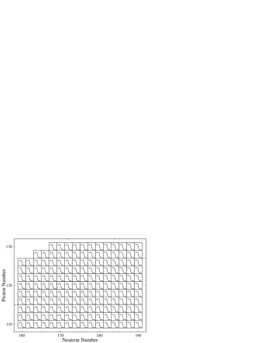
FIG. 12.: Distribution of the mass density from spherical calculations with SkI3 in the region of the $Z=120$, $N=172$, and $N=184$ shells.

The details of this effect as they appear in the non-relativistic SkI3 are shown quantitatively in Fig. 11 for selected neutron (left) and proton states (right), in both cases one level with large and one with small orbital angular momentum close to the Fermi energy. The upper panels show the radial density distributions $4\pi\,r^{2}\,|\phi(r)|$ of the $2g$ and $3d$ neutron states and $2f$ and $3p$ proton states, where $\phi(r)$ is the radial component of the single-particle wavefunction $\psi(\bf{r})$. The radial density is shown for the state with larger total angular momentum only. The middle panels shows the integrand $r\,W_{q,r}\,(\ell+{\textstyle\frac{1}{2}})[(\ell+{\textstyle\frac{3}{2}})|\phi_{\ell+1/2}|^{2}-(\ell-{\textstyle\frac{1}{2}})|\phi_{\ell-1/2}|^{2}]$ which enters the calculation of the spin-orbit splitting (10), while the radial component of the spin-orbit potential $W_{r}$ is shown in the lower panels. Besides the familiar attractive peak at the surface of the nucleus, the central depression of the density leads to a repulsive peak of the spin-orbit potential around $r\approx 3\;{\rm fm}$. The total spin-orbit splitting now depends sensitively on the location of the radial wavefunctions. The neutron $3d$ and proton $3p$ states with three nodes but small angular momentum have large overlap with both the repulsive and the attractive part of the spin-orbit potential (note that small radii are supressed only with $1/r$ and not as usual with $1/r^{2}$), leading to nearly vanishing spin-orbit splitting, while the neutron $2g$ and proton $2f$ states with only two nodes feel only the spin-orbit potential at the nuclear surface (and have much larger overlap with this than the small-angular-momentum states), showing the usual spin-orbit splitting.

Note that this is a polarization effect that is naturally included in the self-consistent description of nuclei but cannot occur in semi-microscopic approaches like the “Extended Thomas-Fermi-Strutinski Integral” method (ETFSI) [76, 77] or macroscopic-microscopic models [69] with prescribed densities and/or single-particle potentials, where one has a very restricted variational freedom of the density profile only (ETFSI) or no degree-of-freedom in the density distribution and single-particle potentials at all (macroscopic-microscopic). Looking at the spectrum calculated with the FY model, the spin-orbit splitting is indeed much larger than in self-consistent models, especially for the $3p$ proton and $2g$ neutron states which are crucial for the $N=172$ shell closure. Comparing Fig. 9 with Fig. 4 for ${}^{298}{114}$ one immediatley sees that the change in the single-particle spectra of both protons and neutrons predicted by FY is much smaller when going from ${}^{298}{114}$ to ${}^{292}{120}$ than in all self-consistent models.

Figure 12 shows the profile of the total density in even-even nuclei in the region of the $Z=120$, $N=172$ and $N=184$ shells as they result from spherical calculations with SkI3. This demonstrates that the density profiles are coupled to the shell closures (and vice versa). At large neutron numbers $N>184$ all nuclei have the usual density profiles, while going below $N=184$ the nuclei immeadiately show a central depression that is most pronounced for nuclei with $Z=120$. It is noteworthy from Fig. 12 that the central depression of the density distribution is coupled to the neutron number – it disappears for all neutron numbers above $N=184$, while the density profiles of nuclei with constant neutron number but different proton number look very similar. The reason for this is that the last filled neutron levels below the $N=172$ gap – $2g_{9/2^{+}}$ and $1j_{15/2^{-}}$ and $2g_{7/2^{+}}$ – all have large orbital angular momentum and are therefore mainly located at the nuclear surface. Going from $N=172$ to $N=184$ only levels with small angular momentum – $3d_{5/2^{+}}$, $3d_{3/2^{+}}$ and $4s_{1/2^{+}}$ – are occupied which have a large probability distribution at small radii. This means that the unusual density distribution of nuclei around ${}^{292}_{172}120$ is simply caused by the filling of the neutron levels which have the same ordering in all models investigated here. This effect thus should occur in non-self-consistent models as well. And indeed the densities calculated from the FY model (plotted in the upper panel of Fig. 10) show the same behaviour as the densities from the self-consistent models, although the effect is weaker here. But unlike the non-self-consistent models with prescribed potentials, the densities in self-consistent models are fed back into the potentials which amplifies the effect by driving the wavefunctions to larger radii. Additionally the self-consistent spin-orbit potentials are influenced which in turn causes the $Z=120$ proton shell closure.

FIG. 13.: 1 Single–neutron levels in the vicinity of the Fermi energy for the isotones of $N=172$ versus the proton number, computed with SkI3.

The same effect which creates the $Z=120$ proton shell is responsible for the appearance of a magic neutron number $N=172$. The gap at $N=172$ depends sensitively on the amplitude of the spin-orbit splitting of the $3d$ neutron levels above this gap. Therefore it occurs again only for the RMF parametrisations and the generalized Skyrme functional SkI3. It can be expected that this neutron shell closure is restricted to nuclei with a prominent central depression of the density like the $Z=120$ proton shell closure. Fig. 13 shows the single-particle energies of the neutrons in the chain of $N=172$ isotones calculated with SkI3. The $N=172$ gap is largest for $Z=120$ in agreement with our findings for the $\delta_{\rm 2n}$ in [31]. Although all these $N=172$ isotones show a central depression of the density distribution, for those those around $Z=120$ the decrease in density when going to small radii is steepest. This gives the largest (positive) peak in the spin-orbit potential and therefore the smallest spin-orbit splitting of the neutron $3d$ levels which in turn gives the largest gap in the spectrum.

F The Shell Structure of ${}^{310}_{184}126$

FIG. 14.: Two–proton gap in the chain of $Z=126$ isotones calculated with the parameterizations as indicated.

The question weather $Z=114$ or $Z=126$ is the next spherical shell closure beyond the experimentally known $Z=82$ is as old as the first extrapolations of nuclear shell structure to superheavy nuclei in simple models. While $Z=126$ corresponds to the largest experimentally known magic neutron number, $Z=114$ has no counterpart for the neutrons. A large number of self-consistent models predict $Z=120$ to be the next proton shell closure, but there are some parametrisations predicting $Z=126$ as an alternative.

Figure 14 shows the two-proton shell gap $\delta_{\rm 2p}$ for the chain of $Z=126$ isotopes calculated with the forces as indicated. For SkP and SkM^∗ two Skyrme forces forces which both have a large effective mass this is a major spherical shell closure. As in case of $Z=120$ the shell closure is neutron-number dependent, it fades away when going to neutron numbers beyond $N=184$. For most other Skyrme forces there is only a slight enhancement of $\delta_{\rm 2p}$ in a small vicinity around $N=184$ which cannot be interpreted as a shell closure. The forces with “relativistic” spin-orbit coupling, i.e. all RMF forces and SkI3, predict very small shell gaps only.

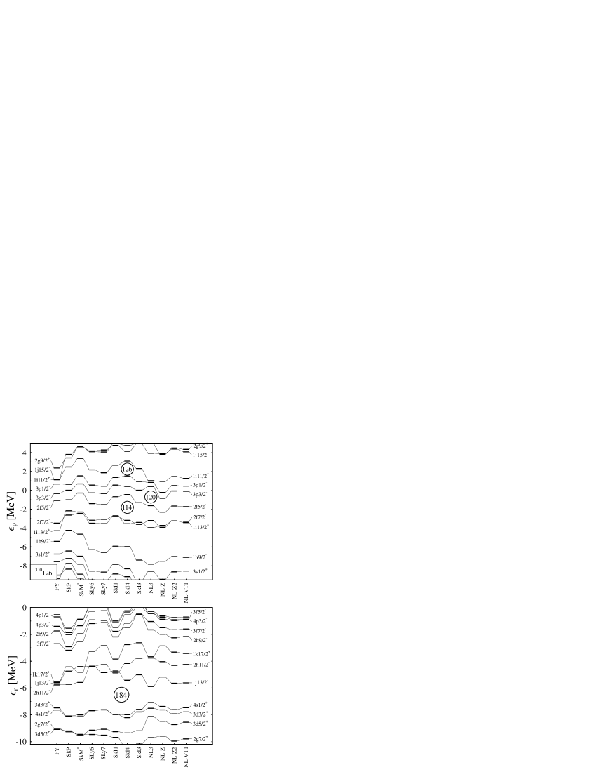
FIG. 15.: The same as in Fig. 4, but for ${}^{310}_{184}126$.

This is reflected in the single-particle spectra, see Fig. 15. Contrary to the appearance of the $Z=114$ and $Z=120$ shell closures, which can be explained simply by looking at the spin-orbit splitting of adjacent proton levels, the situation is more complicated for the $Z=126$ shell closure. The $1i_{11/2^{+}}$ proton state which lies above the $Z=126$ gap is widely separated from the deeply bound $1i_{13/2^{+}}$ state. Therefore the appearance of the magic number $Z=126$ does not depend only on the amplitude of spin-orbit splitting but on the relative distance of levels with different orbital angular momentum as well, although all relativistic forces with overall small spin-orbit splitting show no shell closure at $Z=126$. Remembering that states with large angular momentum have systematically too small single-particle energies and that the spin-orbit splitting predicted by the standard Skyrme forces and SkI4 is too large in heavy nuclei – both would reduce the $Z=126$ gap – the occurrence of a proton shell closure at $Z=126$ is very questionable.

Comparing the single-proton spectra of ${}^{298}_{184}114$ (Fig. 4) and ${}^{310}_{184}126$ one sees immedeatly that the gap at $Z=126$ becomes much smaller with increasing proton number. An exception is the non-selfconsistent FY model, here the relative distances of all proton and neutron have only slightly changed. This gives a further example for the strong dependence of the shell structure of superheavy nuclei on the nucleon numbers in self-consistent models.

For all forces the Fermi energy is positive which means that ${}^{310}_{184}126$ is predicted to be unstable against proton emission. However, owing to the large Coulomb barrier in superheavy nuclei we expect that this nucleus decays trough other more common channels.

G Spin-orbit splitting in superheavy nuclei

We have seen that the predictions of self-consistent models for the spin-orbit splitting in superheavy nuclei shows a pronounced dependence on the nucleon numbers and the orbital angular momentum of the single-particle states. This is summarized in Fig 16. The upper panel shows the spin-orbit splitting of the $3f$ (white markers) and $3p$ (black markers) proton states, while the lower panel shows the splitting of the $2g$ (white markers) and $3d$ (black markers) neutron states in the nuclei as indicated for all forces under investigation. The trivial trend with the orbital angular momentum $\ell$ of the states is removed dividing by $2\ell+1$, see Eq. (10).

While in the non-self-consistent Folded-Yukawa (FY) model all states have nearly the same renormalized spin-orbit splitting, there are large differences between the self-consistent models. The predictions of the forces for certain states in certain nuclei differ as such, but there are clearly visible trends with nucleon number and orbital angular momentum which occur for all parameterizations. Picking out one force, one sees in most cases the same pattern: The spin-orbit splitting of a given state in ${}^{310}_{184}126$ is larger than in ${}^{298}_{184}114$, while it is smallest in ${}^{292}_{172}120$. The (renormalized) splitting of states with large orbital angular momentum is always larger than the splitting of states with small orbital angular momentum. As already discussed above, this is related to the shape of the nuclear density distribution and the effect is largest in ${}^{292}_{172}120$, for which most self-consistent forces predict a pronounced central depression in the density.

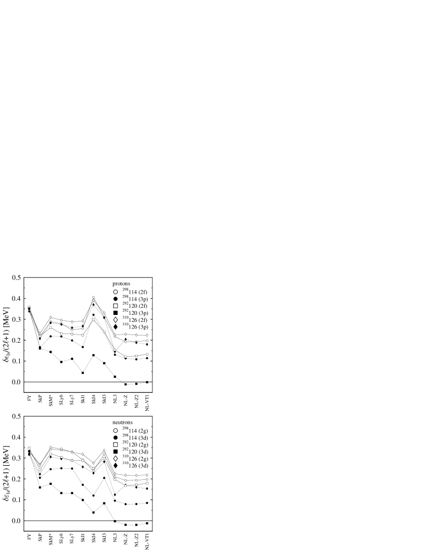
FIG. 16.: Amplitude of the spin–orbit splitting of several superheavy nuclei as predicted by the mean–field forces as indicated. The ls-splitting is weighted with $1/(2\ell+1)$ to remove the trivial dependency on the orbital angular momentum. This shows nicely that in self–consistent models the ls-splitting has an additional state–dependency that does not occur in simple potential models like FY (In the modified oscillator model the splitting is simply the $\kappa$ parameter in the potential) that is related to the shape of the density distribution.

There is a difference between protons and neutrons. While the splitting of the $2g$ neutron state is comparable in all nuclei (although it follows the trend mentioned above), the differences with mass number for the $2f$ proton states is much more pronounced.

There are large differences between the various forces. The parameterizations can be divided into three groups which differ in the isospin dependence of the spin-orbit interaction: standard Skyrme forces (SkP-SkI1), extended Skyrme forces (SkI3, SkI4) and RMF forces (NL3, NL-Z, NL-Z2, and NL-VT1). The standard Skyrme forces in most cases predict larger spin-orbit splittings than the RMF forces. Like in the case of the known nuclei, the predictions of the extended Skyrme forces SkI3 and SkI4 do not stay in between the predictions of standard Skyrme forces and the RMF. Again, SkI3 gives much larger spin-orbit splittings than the RMF forces with a similar isospin dependence of the spin-orbit interaction, while SkI4 stays in betwen standard Skyrme forces and RMF forces for neutrons, but gives the largest splittings for proton levels. For SkP, the force with large effective mass $m^{\ast}/m=1.0$ and the smallest spin-orbit parameter $b_{4}$, the results look somewhat different as it was already the case for the known nuclei discussed in Sect. V B, the spin-orbit splitting of the large angular momentum states and the dependence of the amplitude of the renormalized spin-orbit splitting on the orbital angular momentum is smaller than in other standard Skyrme forces.

The predictions for shell closures are sensitive on the isospin dependence of the spin-orbit interaction and the isoscalar effective mass. But there are additional dependencies of the spin-orbit splitting than the already mentioned ones as can be seen by comparing SkI3 and the RMF forces, which have similar effective mass and isospin dependence of the spin-orbit interaction.

VI Summary and conclusions

We have investigated the influence of the isospin dependence of the spin-orbit force and the effective mass on the predictions for spherical shell closures in superheavy nuclei.

We have introduced two new RMF forces: NL–Z2 and NL–VT1, both employing the standard nonlinear ansatz for the Lagrangian, but NL-VT1 complemented with tensor couplings of the isoscalar and isovector vector fields. Both are fitted to the same set of experimental data as the recent Skyrme parameterizations SkI$x$. The tensor coupling changes the relative distances between the single-particle states, but it has no visible influence on spin-orbit splittings in heavy and superheavy nuclei.

To test the predictive power of the models, we have compared the experimental and calculated single-particle spectra in ${}^{208}{\rm Pb}$, the heaviest known spherical doubly-magic nucleus so far. Already in this nucleus used in the fit of all forces investigated here we see large differences between calculations and experiment and among the forces. States with large angular momentum are shifted to too small single-particle energies and none of the self-consistent models gives the proper level ordering.

The predictions for shell closures are found to be sensitive to the isospin dependence of the spin-orbit interaction and the isoscalar effective mass. The uncertainties of these quantities in the description of smaller nuclei amplify when going to large mass numbers, making predictions for superheavy nuclei a demanding task.

The occurrence of proton shell closures in self-consistent models depends strongly on the neutron number (and vice versa), even when looking at spherical nuclei only. This effect can be explained in terms of single-particle spectra as a coupling of the spin-orbit field to the profile of the density distribution (of protons and neutrons separately) which undergoes dramatic changes in superheavy nuclei. This is an effect of self-consistency, it cannot occur in models where the density distribution has only a restricted degree of freedom like the semi-microscopic ETFSI approach or has even no degree-of-freedom at all like in case of macroscopic-microscopic models. In the region around ${}^{292}_{172}120$ all forces with small effective mass predict a deep central depression of the nuclear density, which induces an unusual shape of the spin-orbit potential that causes an additional state-dependence of the spin-orbit splitting. In some cases the usual level ordering of spin-orbit coupled states is even reverted.

The change of the single-particle spectra of both protons and neutrons when varying proton and neutron number is much larger in all self-consistent models than in non-self-consistent approaches, which was shown on the example of the Folded-Yukawa model.

The only self-consistent force which predicts $Z=114$ for the next spherical magic proton number is the extended Skyrme force SkI4. Although SkI4 gives a very good description of the binding energies in known (deformed) superheavy nuclei [32] and reproduces the kink in the isotopic shifts of the mean-square radii in heavy lead nuclei, it overestimates the spin-orbit splittings of proton states in heavy nuclei by $60-80\%$. This discrepancy between this very good description of bulk properties and a rather poor description of details of the single-particle spectra is yet to be understood. Since a possible proton shell closure at $Z=114$ is caused by a large spin-orbit splitting, the unique prediction of SkI4 is very questionable. On the other hand, all RMF forces, which are in very good agreement with experimental data for spin-orbit splittings throughout the chart of nuclei predict a magic $Z=120$.

In summary this gives a strong argument that the next magic proton number is $Z=120$, coupled with a magic neutron number $N=172$, still a far way to go from the heaviest presently known nucleus ${}^{277}_{165}112$.

A Details of the Mean-Field Models

1 The Skyrme Energy Functional

TABLE II.: Parameters of the Skyrme energy interactions. The $t_{i}$, $x_{i}$, $b_{4}$, $b_{4}^{\prime}$ and $\alpha$ are the parameters of the Skyrme functional (A7), $\hbar^{2}/2m$ is the constant in the calculation of the kinetic energy (A3).

Parameter	SkM*	SkP	SkI1	SkI3	SkI4	SLy6	SLy7
$t_{0}$ $[{\rm MeV}\;{\rm fm}^{3}]$	$-2645.0$	$-2931.70$	$-1913.619$	$-1762.88$	$-1855.827$	$-2479.50$	$-2480.80$
$t_{1}$ $[{\rm MeV}\;{\rm fm}^{5}]$	410.0	320.662	439.809	561.608	473.829	462.180	461.290
$t_{2}$ $[{\rm MeV}\;{\rm fm}^{5}]$	$-135.0$	$-337.41$	2697.594	$-227.090$	1006.855	$-448.610$	$-433.930$
$t_{3}$ $[{\rm MeV}\;{\rm fm}^{3+\alpha}]$	15595.0	18708.97	10592.267	8106.2	9703.607	13673.0	13669.0
$x_{0}$	0.09	0.29215	$-0.954536$	0.3083	0.405082	0.825	0.848
$x_{1}$	0.0	0.65318	$-5.782388$	$-1.1722$	$-2.889148$	$-0.465$	$-0.492$
$x_{2}$	0.0	$-0.53732$	$1.287379$	$-1.0907$	$1.325150$	$-1.0$	$-1.0$
$x_{3}$	0.0	0.18103	$-1.561421$	1.2926	$1.145203$	1.355	1.393
$b_{4}$ $[{\rm MeV}\;{\rm fm}^{4}]$	65.0	50.0	62.130	94.254	183.097	61.0	62.5
$b_{4}^{\prime}$ $[{\rm MeV}\;{\rm fm}^{4}]$	65.0	50.0	62.130	0.0	$-180.351$	61.0	62.5
$\alpha$	$1/6$	$1/6$	0.25	0.25	0.25	$1/6$	$1/6$
$\hbar^{2}/2m$ $[{\rm MeV}\;{\rm fm}^{2}]$	20.733983	0.733983	20.7525	20.7525	20.7525	20.73552985	20.73552985

The Skyrme energy functionals are constructed to be effective interactions for nuclear mean-field calculations. For even-even nuclei, the Skyrme energy functional used in this paper

$${\cal E}={\cal E}_{\rm kin}[\tau]+{\cal E}_{\rm Sk}[\rho,\tau,{\bf J}]+{\cal E}_{\rm C}[\rho_{p}]-{\cal E}_{\rm cm}\quad,$$ (A1)

is composed of the functional of the kinetic energy ${\cal E}_{\rm kin}$, the effective functional for the strong interaction ${\cal E}_{\rm Sk}$ and the Coulomb interaction ${\cal E}_{\rm C}$ including the exchange term in Slater approximation, and the correction for spurious center-of-mass motion ${\cal E}_{\rm cm}$. The energy functionals are the spatial integrals of the corresponding Hamiltonian densities ${\cal H}$

$${\cal E}[\rho,\tau,{\bf J}]=\int\!{\rm d}^{3}r\;{\cal H}[\rho({\bf r}),\tau({\bf r}),{\bf J}({\bf r})]\quad.$$ (A2)

The actual functionals are given by

$${\cal H}_{\rm kin} = \frac{\hbar^{2}}{2m}\tau$$ (A3)

$${\cal H}_{\rm C} = \frac{e^{2}}{2}\int\!{\rm d}^{3}r^{\prime}\frac{\rho_{\rm p}(\textbf{r})\rho_{\rm p}(\textbf{r}^{\prime})}{|\textbf{r}-\textbf{r}^{\prime}|}-\frac{3e^{2}}{4}\left(\frac{3}{\pi}\right)^{1/3}\!\!\rho_{\rm p}^{4/3}$$ (A4)

$${\cal H}_{\rm Sk} = \frac{b_{0}}{2}\rho^{2}+b_{1}\rho\tau-\frac{b_{2}}{2}\rho\Delta\rho+\frac{b_{3}}{3}\rho^{\alpha+2}$$ (A7)

$$-\sum_{q}\bigg{[}\frac{b^{\prime}_{0}}{2}\rho_{q}^{2}+b^{\prime}_{1}\rho_{q}\tau_{q}-\frac{b^{\prime}_{2}}{2}\rho_{q}\Delta\rho_{q}+\frac{b^{\prime}_{3}}{3}\rho^{\alpha}\rho_{q}^{2}\bigg{]}$$

$$+{\cal H}_{\rm LS}$$

with various possibilities for the spin-orbit interaction

$${\cal H}_{\rm LS}^{({\rm std})} = -b_{4}\Big{(}\rho\nabla\cdot{\bf{J}}+\sum_{q}\rho_{q}\nabla\cdot{\bf J}_{q}\Big{)}\quad,$$ (A8)

$${\cal H}_{\rm LS}^{({\bf J})} = {\cal H}_{\rm LS}^{({\rm std})}+c_{1}{\bf J}^{2}-c_{1}^{\prime}\sum_{q}{\bf J}^{2}_{q}\quad,$$ (A9)

$${\cal H}_{\rm LS}^{({\rm ext})} = -b_{4}\;\rho\nabla\cdot{\bf{J}}-b^{\prime}_{4}\sum_{q}\rho_{q}\nabla\cdot{\bf J}_{q}\quad.$$ (A10)

${\cal H}_{\rm LS}^{({\rm std})}$ is reproduced from ${\cal H}_{\rm LS}^{({\rm ext})}$ setting $b^{\prime}_{4}=b_{4}$.

TABLE III.: Parameters of the RMF forces used in this investigation. The mass of the isovector vector-field ${m_{\rho}=763\ {\rm MeV}}$ is not fitted and is the same for all forces.

Force	$m_{N}$	$m_{\sigma}$	$m_{\omega}$	$g_{\sigma}$	$g_{\omega}$	$g_{\rho}$	$b_{2}$	$b_{3}$
	$(MeV)$	$(MeV)$	$(MeV)$			$(fm^{-1})$
NL3	$939.0$	$508.194$	$782.501$	$10.2170$	$12.8680$	$4.47400$	$-10.4310$	$-28.8850$
NL-Z	$938.9$	$488.67$	$780.0$	$10.0553$	$12.9086$	$4.84944$	$-13.5072$	$-40.2243$
NL-Z2	$938.9$	$493.150$	$780.0$	$10.1369$	$12.9084$	$4.55627$	$-13.7561$	$-41.4013$
NL-VT1	$938.9$	$484.307$	$780.0$	$9.81307$	$12.6504$	$4.63432$	$-13.2808$	$-38.0773$	$f_{\omega}/g_{\omega}=-0.102703$
									$f_{\rho}/g_{\rho}=-4.71143$

The local density $\rho_{q}$, kinetic density $\tau_{q}$ and spin-orbit current ${\bf J}_{q}$ entering the functional are given by

$$\rho_{q} = \sum_{k\in\Omega_{q}}v_{k}^{2}\;|\psi_{k}|^{2}\quad,$$ (A11)

$$\tau_{q} = \sum_{k\in\Omega_{q}}v_{k}^{2}\;|\nabla\psi_{k}|^{2}\quad,$$ (A12)

$${\bf J}_{q} = -{\textstyle\frac{i}{2}}\sum_{k\in\Omega_{q}}v_{k}^{2}\;\Big{[}\psi_{k}^{\dagger}\,\nabla\times\hat{\sigma}\,\psi_{k}-(\nabla\times\hat{\sigma}\,\psi_{k})^{\dagger}\psi_{k}\Big{]}\quad,$$ (A13)

with $q\in\{p,n\}$. Densities without index denote total densities, e.g. $\rho=\rho_{\rm p}+\rho_{\rm n}$. The $\psi_{k}$ are the single-particle wavefunctions and $v_{k}^{2}$ the occupation probabilities calculated taking the residual pairing interaction into account, see Appendix A 3. The parameters $b_{i}$ and $b^{\prime}_{i}$ used in the above definition are chosen to give a most compact formulation of the energy functional, the corresponding mean-field Hamiltonian and residual interaction [78]. They are related to the more commonly used Skyrme force parameters $t_{i}$ and $x_{i}$ by

$$b_{0} = t_{0}\big{(}1+{\textstyle\frac{1}{2}}x_{0}\big{)}\quad,$$ (A14)

$$b^{\prime}_{0} = t_{0}\big{(}{\textstyle\frac{1}{2}}+x_{0}\big{)}\quad,$$ (A15)

$$b_{1} = {\textstyle\frac{1}{4}}\big{[}t_{1}\big{(}1+{\textstyle\frac{1}{2}}x_{1}\big{)}+t_{2}\big{(}1+{\textstyle\frac{1}{2}}x_{2}\big{)}\big{]}\quad,$$ (A16)

$$b^{\prime}_{1} = {\textstyle\frac{1}{4}}\big{[}t_{1}\big{(}{\textstyle\frac{1}{2}}+x_{1}\big{)}-t_{2}\big{(}{\textstyle\frac{1}{2}}+x_{2}\big{)}\big{]}\quad,$$ (A17)

$$b_{2} = {\textstyle\frac{1}{8}}\big{[}3t_{1}\big{(}1+{\textstyle\frac{1}{2}}x_{1}\big{)}-t_{2}\big{(}1+{\textstyle\frac{1}{2}}x_{2}\big{)}\big{]}\quad,$$ (A18)

$$b^{\prime}_{2} = {\textstyle\frac{1}{8}}\big{[}3t_{1}\big{(}{\textstyle\frac{1}{2}}+x_{1}\big{)}+t_{2}\big{(}{\textstyle\frac{1}{2}}+x_{2}\big{)}\big{]}\quad,$$ (A19)

$$b_{3} = {\textstyle\frac{1}{4}}t_{3}\big{(}1+{\textstyle\frac{1}{2}}x_{3}\big{)}\quad,$$ (A20)

$$b^{\prime}_{3} = {\textstyle\frac{1}{4}}t_{3}\big{(}{\textstyle\frac{1}{2}}+x_{3}\big{)}\quad,$$ (A21)

$$c_{1} = -{\textstyle\frac{1}{8}}(t_{1}x_{1}+t_{2}x_{2})\quad,$$ (A22)

$$c^{\prime}_{1} = -{\textstyle\frac{1}{8}}(t_{1}-t_{2})\quad,$$ (A23)

The actual parameters for the parameterizations used in this paper are summarized in Table II.

The single-particle Hamiltonian is derived variationally from the energy functional. One obtains

$$\hat{h}_{q}=-\nabla\cdot B_{q}\nabla+U_{q}-i{\bf W}_{q}\cdot\nabla\times\hat{\sigma}$$ (A24)

with the mean fields

$$B_{q}=\frac{\delta{\cal E}}{\delta\tau_{q}}\quad,\quad U_{q}=\frac{\delta{\cal E}}{\delta\rho_{q}}\quad,\quad{\bf W}_{q}=\frac{\delta{\cal E}}{\delta{\bf J}_{q}}\quad.$$ (A25)

For all forces, a center-of-mass correction is employed. For the SkI$x$ and SLy$x$ forces it is calculated perturbatively by subtracting

$${\cal E}_{\rm cm}=\frac{1}{2mA}\langle\hat{\textbf{P}}\rule{0.0pt}{6.8pt}^{2}_{\rm cm}\rangle$$ (A26)

from the Skyrme functional after the convergence of the Hartree-Fock equations, while for SkM* and SkP only the diagonal direct terms in (A26) are considered self-consistently in the variational equation [49]. For all but the SLy$x$ forces this is the procedure used in the original fit. For SLy6 and SLy7 the microscopic correction (A26) was considered in the variational equations and therefore giving a contribution to the single-particle energy. However, for large nuclei as discussed here the contribution of (A26) to the single-particle energies is negligible because the matrix elements are weighted with $1/(2mA)$ compared to the contributions from the energy functional. We have therefore omitted this feature and follow the suggestion of [45] to use the perturbatively calculated correction from (A26) instead.

2 Relativistic Mean-Field Model

For the sake of a covariant notation, it is better to provide the basic functional in the relativistic mean-field model as an effective Lagrangian ${\cal L}$. For the present version of the RMF used in this study, we can summarize it as

$${\cal L}_{\rm RMF}={\cal L}_{\rm N}+{\cal L}_{\rm M}+{\cal L}_{\rm NM}+{\cal L}_{\rm nonl}+{\cal L}_{\rm em}\quad,$$ (A27)

where ${\cal L}_{\rm N}$ is the free Dirac Lagrangian for the nucleons with nucleon mass $m_{\rm N}$, equally for protons and neutrons

$${\cal L}_{\rm N}=\sum_{k\in\Omega}v_{k}^{2}\;\bar{\psi}_{k}\left(i\gamma_{\mu}\partial^{\mu}-m_{\rm N}\right)\psi_{k}\quad.$$ (A28)

The Lagrangians of the fields and their couplings to the nucleons are given by

$${\cal L}_{\rm M} = {\textstyle\frac{1}{2}}(\partial_{\mu}\Phi_{\sigma}\partial^{\mu}\Phi_{\sigma}-m_{\sigma}^{2}\Phi^{2})$$ (A31)

$$-{\textstyle\frac{1}{2}}\Big{[}{\textstyle\frac{1}{2}}(\partial_{\mu}\Phi^{\mbox{}}_{\omega,\nu}-\partial_{\nu}\Phi^{\mbox{}}_{\omega,\mu})\;\partial^{\mu}\Phi_{\omega}^{\nu}-m_{\omega}^{2}\Phi_{\omega,\mu}^{\mbox{}}\Phi_{\omega}^{\mu}\Big{]}$$

$$-{\textstyle\frac{1}{2}}\Big{[}{\textstyle\frac{1}{2}}(\partial_{\mu}\vec{\Phi}^{\mbox{}}_{\rho,\nu}-\partial_{\nu}\vec{\Phi}^{\mbox{}}_{\rho,\mu})\cdot\partial^{\mu}\vec{\Phi}_{\rho}^{\nu}-m_{\omega}^{2}\vec{\Phi}_{\rho,\mu}^{\mbox{}}\cdot\vec{\Phi}_{\rho}^{\mu}\Big{]}$$

$${\cal L}_{\rm NM} = -g_{\sigma}\Phi_{\sigma}\rho_{\rm s}-g_{\omega}\Phi_{\omega,\mu}\rho^{\mu}-g_{\rho}\vec{\Phi}_{\rho,\mu}\cdot\vec{\rho}^{\,\mu},$$ (A32)

$${\cal L}_{\rm nonl} = {\cal U}_{\sigma\sigma}[\Phi_{\sigma}],$$ (A33)

$${\cal L}_{\rm em} = -{\textstyle\frac{1}{4}}F_{\mu\nu}F^{\mu\nu}-eA_{\mu}\rho_{p}^{\mu},$$ (A34)

The model includes couplings of the scalar-isoscalar ($\Phi_{\sigma}$), vector-isoscalar ($\Phi_{\omega,\mu}$), vector-isovector ($\vec{\Phi}_{\rho,\mu}$), and electro-magnetic ($A_{\mu}$) field to the corresponding scalar-isoscalar ($\rho_{\rm s}$), vector-isoscalar ($\rho^{\mu}$) and vector-isovector ($\vec{\rho}^{\mu}$) densities of the nucleons as well as the proton density $\rho_{p}^{\mu}$, which are defined as

$$\rho_{\rm s} = \sum_{k\in\Omega}v_{k}^{2}\;\bar{\psi}_{k}\psi_{k},$$ (A35)

$$\rho^{\mu} = \sum_{k\in\Omega}v_{k}^{2}\;\bar{\psi}_{k}\gamma_{\mu}\psi_{k},$$ (A36)

$$\vec{\rho}^{\,\mu} = \sum_{k\in\Omega}v_{k}^{2}\;\bar{\psi}_{k}\vec{\tau}\gamma_{\mu}\psi_{k},$$ (A37)

$$\rho_{p}^{\mu} = \sum_{k\in\Omega_{p}}v_{k}^{2}\;\bar{\psi}_{k}\gamma_{\mu}\psi_{k}.$$ (A38)

${\cal U}_{\sigma\sigma}$ is the nonlinear selfinteraction of the scalar-isoscalar field. All forces used in this paper employ the standard ansatz [36]

$${\cal U}_{\sigma\sigma}=-{\textstyle\frac{1}{3}}b_{3}\Phi_{\sigma}^{3}-{\textstyle\frac{1}{4}}b_{4}\Phi_{\sigma}^{4}.$$ (A39)

In case of the parameterset NL-VT1 also a tensor coupling between the nucleons and the vector fields is considered, which can be written as

$${\cal L}_{\rm NM}^{\rm t}=\frac{f_{\omega}}{2m_{\rm N}}\Phi_{\omega,\mu}\rho_{\rm t}^{\mu}+\frac{f_{\rho}}{2m_{\rm N}}\vec{\Phi}_{\rho,\mu}\cdot\vec{\rho}_{\rm t}^{\,\mu}$$ (A40)

with the densities

$$\rho_{\rm t}^{\mu} = \partial_{\nu}\sum_{k\in\Omega}v_{k}^{2}\bar{\psi}_{k}\sigma^{\mu\nu}\psi_{k},$$ (A41)

$$\vec{\rho}_{\rm t}^{\,\mu} = \partial_{\nu}\sum_{k\in\Omega}v_{k}^{2}\bar{\psi}_{k}\sigma^{\mu\nu}\vec{\tau}\psi_{k},$$ (A42)

where $\sigma^{\mu\nu}=(i/2)[\gamma^{\mu},\gamma^{\nu}]$. The masses $m_{i}$ and coupling constants of the fields are the free parameters of the RMF which have to be adjusted to experimental data. The actual parameters of the parameterizations used here are given in Table III. The equation of motion of the single-particle states is derived from a variational principle

$$\epsilon_{k}\gamma_{0}\psi_{k}=\Big{[}-i{\boldmath\gamma}\cdot\nabla+m_{\rm N}+{\cal S}+\gamma_{\mu}{\cal V}^{\mu}\Big{]}\psi_{k}$$ (A43)

where ${\cal S}=g_{\sigma}\Phi_{\sigma}$ and ${\cal V}_{\mu}=g_{\omega}\Phi_{\omega,\mu}+{\textstyle\frac{1}{2}}g_{\rho}\vec{\Phi}_{\rho,\mu}\cdot\vec{\tau}+{\textstyle\frac{1}{2}}eA_{\mu}(1+\tau_{0})$ are the scalar and vector field respectively. A more detailed description of the model can be found in [36].

For the residual pairing interaction and the center-of-mass correction the same non-relativistic approximation is used as in the SHF model, for NL-Z, NL-Z2 and NL-VT1 by subtracting perturbatively the full microscopic correction (A26), while for NL3 the harmonic oscillator estimate $E_{\rm c.m.}=\frac{3}{4}\;41A^{-1/3}\;{\rm MeV}$ is subtracted as done in the fit of these parameter sets.

3 Pairing Energy Functional

TABLE IV.: Pairing strength $V_{\rm n}$ for the neutrons and $V_{\rm p}$ for the protons for the mean–field forces used in this study. $m^{\ast}/m$ is the isoscalar effective mass in infinite nuclear matter. Note that the absolute value of the pairing strength decreases with increasing effective mass.

Force	$m^{\ast}/m$	$V_{\rm n}$ [MeV fm3]	$V_{\rm p}$ [MeV fm3]
SkM*	$0.789$	$-276$	$-292$
SkP	$1.0$	$-241$	$-265$
SkI1	$0.693$	$-320$	$-305$
SkI3	$0.574$	$-340$	$-351$
SkI4	$0.650$	$-310$	$-324$
SLy6	$0.689$	$-308$	$-320$
SLy7	$0.688$	$-308$	$-320$
NL3	$0.595$	$-329$	$-342$
NL-Z	$0.583$	$-349$	$-351$
NL-Z2	$0.583$	$-343$	$-350$
NL-VT1	$0.600$	$-340$	$-346$

Pairing is treated in BCS approximation using a delta pairing force [79, 80], leading to the pairing energy functional

$${\cal E}_{\rm pair}=\frac{1}{4}\sum_{q=\{{\rm p,n}\}}V_{q}\int\!{\rm d}^{3}r\;\chi_{q}^{2}\quad,$$ (A44)

where $\chi_{q}=-2\sum_{k\in\Omega_{q}>0}f_{k}u_{k}v_{k}\;|\psi_{k}|^{2}$ is the pairing density including state-dependent cut-off factors $f_{k}$ to restrict the pairing interaction to the vicinity of the Fermi surface [81]. $v_{k}^{2}$ is the occupation probability of the given single-particle state and $u_{k}^{2}=1-v_{k}^{2}$. The strengths $V_{\rm p}$ for protons and $V_{\rm n}$ for neutrons depend on the actual mean-field parameterization. They are optimized by fitting for each parameterization separately the pairing gaps in isotopic and isotonic chains of semi-magic nuclei throughout the chart of nuclei. The actual values can be found in Table IV. The pairing-active space $\Omega_{q}$ is chosen to embrace one additional shell of oscillator states above the Fermi energy with a smooth cutoff weight, see [81] for details.

4 The Folded-Yukawa Single-Particle Potential

We present here only the details needed for our discussion. A more detailed discussion of the parameterization of the potentials can be found in [69] and references therein. The single-particle Hamiltonian of the Folded-Yukawa single-particle model has the same structure as the one of the Skyrme-Hartree-Fock model (A24), but instead of calculating the potentials self-consistently from the actual density distributions, a parameterized guess for the functional form of the potentials is used. The nucleons have an effective mass of $m^{*}/m=1$ without any radial dependence, therefore $B$ is simply given by $B=\hbar^{2}/2m$. The single-particle potential $U$ is calculated from the folding of a Yukawa function with the sharp nuclear surface

$$U_{q}({\bf r})=-\frac{V_{0}}{4\pi a^{3}}\int_{V}\!{\rm d}^{3}r^{\prime}\frac{e^{-|{\bf r}-{\bf r}^{\prime}|/a}}{|{\bf r}-{\bf r}^{\prime}|/a}$$ (A45)

where the integration is performed oder the nuclear volume. Finally, the spin-orbit potential is given by the derivative of the nuclear potential

$${\bf W}_{q}({\bf r})=-\lambda_{q}(A)\left(\frac{\hbar}{2m}\right)^{2}\nabla\,U_{q}$$ (A46)

with the coupling constants $\lambda_{\rm p}=28.0+6.0\;A/240$ and $\lambda_{\rm p}=31.5+4.5\;A/240$.

REFERENCES

- [1] W. D. Myers, W. J. Swiatecki, Nucl. Phys. 81, 1 (1966).
- [2] S. G. Nilsson, C. F. Tsang, A. Sobiczewski, Z. Szymanski, S. Wycech, C. Gustafson, I.–L. Lamm, P. Möller, and B. Nilsson, Nucl. Phys. A131, 1 (1969).
- [3] U. Mosel and W. Greiner, Z. Phys. 222, 261 (1969).
- [4] E. O. Fizet, J. R. Nix, Nucl. Phys. A193, 647 (1972).
- [5] M. Brack, J. Damgård, A. S. Jensen, H. C. Pauli, V. M. Strutinsky, and C. Y. Wong, Rev. Mod. Phys. 44, 320 (1972).
- [6] S. Hofmann, V. Ninov, F. P. Hessberger, P. Armbruster, H. Folger, G. Münzenberg, H. J. Schött, A. G. Popeko, A. V. Yeremin, A. N. Andreyev, S. Saro, R. Janik, and M. Leino, Z. Phys. A350, 277 (1995) and Z. Phys. A350, 281 (1995).
- [7] A. Ghiorso, D. Lee, L. P. Somerville, W. Loveland, J. M. Nitschke, W. Ghiorso, G. T. Seaborg, P. Wilmarth, R. Leres, A. Wydler, M. Nurmia, K. Gregorich, K. Czerwinski, R. Gaylord, T. Hamilton, N. J. Hannink, D. C. Hoffman, C. Jarzynski, C. Kacher, B. Kadkhodayan, S. Kreek, M. Lane, A. Lyon, M. A. McMahan, M. Neu, T. Sikkeland, W. J. Swiatecki, A. Türler, J. T. Walton, and S. Yashita, Nucl. Phys. A583, 861c (1995); Phys. Rev. C51, R2293 (1995).
- [8] S. Hofmann, V. Ninov, F. P. Hessberger, P. Armbruster, H. Folger, G. Münzenberg, H. J. Schött, A. G. Popeko, A. V. Yeremin, S. Saro, R. Janik, and M. Leino, Z. Phys. A354, 229 (1996).
- [9] Yu. A. Lazarev, Yu. V. Lobanov, Yu. Ts. Oganessian, V. K. Utyonkov, F. Sh. Abdullin, A. N. Polyakov, J. Rigol, I. V. Shirokovsky, Yu. S. Tsyganov, S. Iliev, V. G. Subbotin, A. M. Sukhov, G. V. Buklanov, B. N. Gikal, V. B. Kutner, A. N. Mezentsev, K. Subotic, J. F. Wild, R. W. Lougheed, and K. J. Moody, Phys. Rev. C 54, 620 (1996).
- [10] S. Hofmann, Rep. Prog. Phys. 61, 639 (1998).
- [11] A. Sobiczewski, Z. Patyk, and S. Ćwiok, Phys. Lett. 186, 6 (1987).
- [12] A. Sobiczewski, Z. Patyk, and S. Ćwiok, Phys. Lett. 224, 1 (1989).
- [13] Z. Patyk, A. Sobiczewski, P. Armbruster, and K.–H. Schmidt, Nucl. Phys. A491, 267 (1989).
- [14] Z. Patyk and A. Sobiczewski, Nucl. Phys. A533, 132 (1991).
- [15] P. Möller and J. R. Nix, Nucl. Phys. A549, 84 (1992).
- [16] P. Möller and J. R. Nix, J. Phys. G20, 1681 (1994).
- [17] Yu. A. Lazarev, Yu. V. Lobanov, Yu. S. Oganessian, V. K. Utyonkov, F. Sh. Abdulin, G. V. Buklanov, B. N. Gikal, S. Iliev, A. N. Mezentsev, V. N. Polyakov, I. M. Sedykh, I. V. Shirokovsky, V. G. Subbotin, A. M. Sukhov, Yu. S. Tsyganov, V. E. Zhuchko, R. W. Lougheed, K. J. Moody, J. F. Wild, E. K. Hulet, and J. H. McQuaid, Phys. Rev. Lett. 73, 624 (1994).
- [18] P. Reiter, T. L. Khoo, C. J. Lister, D. Seweryniak, I. Ahmad, M. Alcorta, M. P. Carpenter, J. A. Cizewski, C. N. Davids, G. Gervais, J. P. Greene, W. F. Henning, R. V. F. Janssens, T. Lauritsen, S. Siem, A. A. Sonzogni, D. Sullivan, J. Uusitalo, I. Wiedenh ver, N. Amzal, P. A. Butler, A. J. Chewter, K. Y. Ding, N. Fotiades, J. D. Fox, P. T. Greenlees, R.-D. Herzberg, G. D. Jones, W. Korten, M. Leino, and K. Vetter, Phys. Rev. Lett. 82, 509 (1999).
- [19] S. Ćwiok, V. V. Pashkevich, J. Dudek, and W. Nazarewicz, Nucl. Phys. A410, 254 (1983).
- [20] S. Ćwiok, Z. Łojewski, and V. V. Pashkevich, Nucl. Phys. A444, 1 (1985).
- [21] K. Böning, Z. Patyk, A. Sobiczewski, and S. Ćwiok, Z. Phys. A325, 479 (1986).
- [22] R. Smolańcuk, J. Skalski, und A. Sobiczewski, Phys. Rev. C 52, 1871 (1995).
- [23] D. Vautherin, M. Vénéroni and D. M. Brink, Phys. Lett. B33, 381 (1970).
- [24] M. Beiner, H. Flocard, M. Vénéroni, and P. Quentin, Proceedings of the 27th Nobel Symposium, Super Heavy Elements – Theoretical Predictions and Experimental Generation, Ronneby, Sweden (S. G. Nilsson und N. R. Nilsson, eds.), Physica Scripta 10A, 84 (1974).
- [25] F. Tondeur, Z. Phys. A297, 61 (1980).
- [26] Y. K. Gambhir, P. Ring, and A. Thimet, Ann. Phys. (N.Y.) 198, 132 (1990).
- [27] H. F. Boersma, Phys. Rev. C48, 472 (1993).
- [28] J.–F. Berger, L. Bitaud, J. Dechargé, M. Girod, and S. Peru–Dessenfants, Proceedings of the International Workshop XXXIV on Gross Properties of Nuclei and Nuclear Exitations, Hirschegg, Austria, January 1996. (H. Feldmeier, J. Knoll, and W. Nörenberg, edts.) Gesellschaft für SChwerionenforschung, Darmstadt, 1996, p 56.
- [29] G. A. Lalazissis, M. M. Sharma, P. Ring, and Y. K. Gambir, Nucl. Phys. A608, 202 (1996).
- [30] S. Ćwiok, J. Dobaczewski, P.–H. Heenen, P. Magierski, and W. Nazarewicz, Nucl. Phys. A611, 211 (1996).
- [31] K. Rutz, M. Bender, T. Bürvenich, T. Schilling, P.–G. Reinhard, J. A. Maruhn, and W. Greiner, Phys. Rev. C 56, 238 (1997).
- [32] T. Bürvenich, K. Rutz, M. Bender, P.–G. Reinhard, J. A. Maruhn, and W. Greiner, EPJ A 3, 139 (1998).
- [33] M. Bender, K. Rutz, P.–G. Reinhard, J. A. Maruhn, and W. Greiner, Phys. Rev. C 58, 2126 (1998).
- [34] P. Quentin and H. Flocard, Ann. Rev. Nucl. Part. Sci. 28, 523 (1978).
- [35] B. D. Serot and J. D. Walecka, Adv. Nucl. Phys. 16, 1 (1986).
- [36] P.–G. Reinhard, Rep. Prog. Phys. 52, 439 (1989).
- [37] P. Ring, Prog. Part. Nucl. Phys. 37, 193 (1996).
- [38] J. Dechargé and D. Gogny, Phys. Rev. 21, 1568 (1980).
- [39] P. Hohenberg and W. Kohn, Phys. Rev. B136, 864 (1964).
- [40] W. Kohn, L. J. Sham, Phys. Rev. A 140, 1133 (1965).
- [41] P.–G. Reinhard and C. Toepffer, Int. J. of Mod. Phys. E3, 435 (1994).
- [42] J. Bartel, P. Quentin, M. Brack, C. Guet, and H.–B. Håkansson, Nucl. Phys. A386, 79 (1982).
- [43] J. Dobaczewski, H. Flocard, and J. Treiner, Nucl. Phys. A422, 103 (1984).
- [44] E. Chabanat, Interactions effectives pour des conditions extrêmes d’isospin, Université Claude Bernard Lyon-1, Thesis 1995, LYCEN T 9501, unpublished.
- [45] E. Chabanat, P. Bonche, P. Haensel, J. Meyer, and R. Schaeffer, Nucl. Phys. A635, 231 (1998).
- [46] P.–G. Reinhard and H. Flocard, Nucl. Phys. A584, 467 (1995).
- [47] G. A. Lalazissis, J. König, and P. Ring, Phys. Rev. C 55, 540 (1997).
- [48] M. Rufa, P.–G. Reinhard, J. A. Maruhn, W. Greiner, and M. R. Strayer, Phys. Rev. C 38, 390 (1989).
- [49] J. Friedrich and P.–G. Reinhard, Phys. Rev. C 33, 335 (1986).
- [50] J. P. Blaizot, Phys. Rep. 64, 171 (1980).
- [51] M. Brack, C. Guet, H.-B. Hakansson, Phys.Rep. 123, 275 (1985).
- [52] V. Blum, G. Lauritsch, J. A. Maruhn, and P.–G. Reinhard, J. Comp. Phys. 100, 364 (1992).
- [53] O. Haxel, J. H. D. Jensen and H. E. Suess, Phys. Rev. 75, 1766 (1949).
- [54] M. Goeppert Mayer, Phys. Rev. 75, 1969 (1949).
- [55] S. G. Nilsson and I. Ragnarsson, Shapes and shells in nuclear structure, Cambridge University Press, Cambridge, 1995.
- [56] H. P. Duerr, Phys. Rev. 103, 469 (1956).
- [57] J. S. Bell and T. H. R. Skyrme, Philosophical Magazine 1, 1055 (1965).
- [58] T. H. R. Skyrme, Nucl. Phys. 9, 635 (1959).
- [59] G. A. Lalazissis, M. M. Sharma, J. König, and P. Ring, International Conference on “Nuclear Shapes and Nuclear Structure at Low Excitation Energies”, Antibes (France) June 20–25, 1994 (Gif–sur–Yvette Cedex, France) (M. Vergnes, D. Goutte, P.–H. Heenen, und J. Sauvage, eds.), Editions Frontieres, 1994, p. 161.
- [60] M. M. Sharma, G. A. Lalazissis, J. König, and P. Ring, Phys. Rev. Lett. 74, 3744 (1995).
- [61] M. Bolsterli, E. O. Fiset, J. R. Nix, and J. L. Norton, Phys. Rev. C 5, 1050 (1972).
- [62] W. Nazarewicz, J. Dudek, R. Bengtsson, T. Bengtsson, and I. Ragnarsson, Nucl. Phys. A 435, 397 (1985).
- [63] J. Dobaczewski, W. Nazarewicz, and T. R. Werner, Phys. Scr. T56, 15 (1995).
- [64] M. Jaminon and C. Mahaux, Phys. Rev. C 40, 354 (1989).
- [65] K. Rutz, M. Bender, P.–G. Reinhard, J. A. Maruhn, and W. Greiner, Nucl. Phys. A634, 67 (1998).
- [66] R. R. Kinsey et al., The NUDAT/PCNUDAT Program for Nuclear Data, 9th International Symposium of Capture Gamma–Ray Spectroscopy and Related Topics (Budapest, Hungary, October 1996). Data extracted from the NUDAT database, version March 20, 1997, National Nuclear Data Center WorldWideWeb site.
- [67] M. Bender, T. Bürvenich, K. Rutz, J. A. Maruhn, W. Greiner, and P.–G. Reinhard, Proceedings of the International Workshop XXXVI on Gross Properties of Nuclei and Nuclear Exitations, Hirschegg, Austria, January 11–17 1998, (M. Buballa, W. Nörenberg, J. Wambach, A. Wirzba, eds.) Gesellschaft für Schwerionenforschung, Darmstadt, 1998, p. 59.
- [68] M. Bender, K. Rutz, T. Bürvenich, P.–G. Reinhard, J. A. Maruhn, and W. Greiner, Proceedings of the Nuclear Structure ’98 International Conference, Gatlinburg, Tennessee, August 10–15 1998. (to be published)
- [69] P. Möller, J. R. Nix, W. D. Myers, and W. J. Swiatecki, At. Data Nucl. Data Tables 59, 185 (1995).
- [70] M. Lewitowicz, Yu. E. Penionzhkevich, A. G. Artukh, A. M. Kalinin, V. V. Kamanin, S. M. Lukyanov, Nguyen Hoai Chau, A. C. Mueller, D. Guillemaud–Mueller, R. Anne, D. Bazin, C. Detraz, D. Guerreau, M. G. Saint–Laurent, V. Borrel, J. C. Jacmart, F. Pougheon, A. Richard, W. D. Schmidt–Ott, Nucl. Phys. A496, 477 (1989).
- [71] O. Sorlin, D. Guillemaud–Mueller, A. C. Mueller, V. Borrel, S. Dogny, F. Pougheon, K.–L. Kratz, H. Gabelmann, B. Pfeiffer, A. Wohr, W. Ziegert, Yu. E. Penionzhkevich, S. M. Lukyanov, V. S. Salamatin, R. Anne, C. Borcea, L. K. Fifield, M. Lewitowicz, M. G. Saint–Laurent, D. Bazin, C. Detraz, F.–K. Thielemann, and W. Hillebrandt, Phys. Rev. C 47, 2941 (1993).
- [72] H. Scheit, T. Glasmacher, B. A. Brown, J. A. Brown, P. D. Cottle, P. G. Hansen, R. Harkewicz, M. Hellstrom, R. W. Ibbotson, J. K. Jewell, K. W. Kemper, D. J. Morrissey, M. Steiner, P. Thirolf, and M. Thoennessen, Phys. Rev. Lett. 77, 3967 (1996).
- [73] T. Glasmacher, B. A. Brown, M. J. Chromik, P. D. Cottle, M. Fauerbach, R. W. Ibbotson, K. W. Kemper, D. J. Morrissey, H. Scheit, D. W. Sklenicka, and M. Steiner, Phys. Lett. B 395, 163 (1997).
- [74] T. R. Werner, J. A. Sheikh, M. Misu, W. Nazarewicz, J. Rikovska, K. Heeger, A. S. Umar, and M. R. Strayer, Nucl. Phys. A597, 327 (1996) and work cited therein.
- [75] G. A. Lalazissis, D. Vretanar, P. Ring, M. Stoitsov, and L. Robledo, preprint nucl-th/9807029.
- [76] J. M. Pearson, Y. Aboussir, A. K. Dutta, R. C. Nayak, M. Farine, and F. Tondeur, Nucl. Phys. A528, 1 (1991).
- [77] Y. Aboussir, J. M. Pearson, A. K. Dutta, and F. Tondeur, At. Data Nucl. Data Tables 61, 127 (1995).
- [78] P.–G. Reinhard, Ann. Phys. (Leipzig) 1, 632 (1992).
- [79] F. Tondeur, Phys. Lett. 123B, 139 (1983).
- [80] S. J. Krieger, P. Bonche, H. Flocard, P. Quentin, and M. S. Weiss, Nucl. Phys. A517, 275 (1990).
- [81] M. Bender, P.–G. Reinhard, K. Rutz, and J. A. Maruhn, preprint, submitted to Phys. Rev. C (1998).