Abstract

Using a chiral unitary model in which the negative parity nucleon resonance $N^{\ast}\equiv N^{\ast}(1535)$ is generated dynamically by means of the Bethe Salpeter equation with coupled meson baryon channels in the $S=0$ sector, we have obtained the $\pi^{0}N^{\ast}N^{\ast}$ and $\eta N^{\ast}N^{\ast}$ couplings. The $\pi^{0}N^{\ast}N^{\ast}$ coupling has smaller strength but the same sign as the $\pi^{0}NN$ coupling. This rules out the mirror assignment of chiral symmetry where the ground state nucleon $N$ and the negative parity resonance $N^{\ast}$ are envisaged as chiral partners in the baryon sector.

1 Introduction

Chiral symmetry has been playing a crucial role in understanding hadron physics. The current algebra and associated low energy theorems have been successfully applied to hadronic phenomena which in particular involve pions that appear as the Nambu-Goldstone bosons of spontaneous breakdown of chiral symmetry [1]. Recent developments of chiral perturbation methods for mesons and baryons are partly motivated by the hope in the theoretical side to describe hadrons without referring to particular models [2, 3, 4, 5, 6].

In Refs. [7, 8, 9], it was demonstrated that chiral perturbation theories, when unitarization in coupled channels is incorporated, can be applied up to resonance energy regions which are much beyond what the original chiral perturbation theories are supposed to be applied to. In Refs. [7, 8] this approach was referred to as the chiral unitary approach.

The advantage of the use of the chiral unitary approach is based on the implementation of exact unitarity together with a chiral expansion of Re($T^{-1}$) instead of the $T$ matrix, in a way analogous to the effective range expansion in quantum mechanics. These manipulations allow one to extend the information contained in the chiral lagrangians with small number of derivatives to higher energies than expected.

In this way all meson resonances in meson meson scatterings up to 1.2 GeV were obtained [7, 8]. Simultaneously an alternative but equivalent unitary approach was followed in Ref. [10] where the lowest order chiral Lagrangian was explicitly kept and the higher order one was generated from the exchange of genuine QCD resonances, following the idea of Ref. [11]. This allowed one to distinguish between genuine QCD resonances and other resonances which come as a consequence of the scattering of the mesons.

While a great success has been achieved in explaining hadron phenomena, several fundamental questions are not yet clearly answered. Here we would like to raise the following particular one concerning the formation of chiral multiplets: Are there any particles which belong to the same chiral multiplets and so they will get degenerate when chiral symmetry is restored? In a linear sigma model, for instance, of $SU(2)\times SU(2)$ chiral symmetry, a would-be chiral multiplet includes the $\sigma$ and $\pi$ mesons, which are the vector representations of the chiral group. In the spontaneously broken phase the pion becomes massless and the sigma meson remains massive, while in the symmetric phase they get degenerate and acquire an equal mass. Another candidate of a chiral multiplet is the pair of the vector ($\rho$) and axial vector ($a_{1}$) mesons. In both cases, the mass difference between particles in the same multiplet is considered to be generated by a finite scalar condensate associated with spontaneous break down of chiral symmetry.

For baryons, less attention has been paid in identifying them as members of chiral multiplets. For instance, one may ask what would be the chiral partner of the nucleon $N(939)$, and what properties are dictated by the underlying chiral symmetry. In Refs. [12, 13], motivated by these questions, the chiral symmetry of the nucleon has been investigated, where two distinct chiral assignments for baryons were discussed. In one assignment, the positive and negative parity nucleons belong to different chiral multiplets, each of which is an independent representation of chiral symmetry. This case is referred to as the naive assignment. In the other case, positive and negative parity nucleons form a chiral multiplet, in which they transform to each other under chiral transformations. This case is referred to as the mirror assignment.

In both assignments, chiral symmetry puts unique constraints on properties of the positive and negative parity nucleons. In the naive assignment, a chiral symmetric lagrangian reduces to a sum of two lagrangians for positive and negative parity nucleons. Therefore, couplings between them disappear to leading order. In Ref. [13] this fact was considered to be the reason for the small coupling constant $g_{\pi NN^{*}}$ for the decay of $N^{*}=N^{*}(1535)$. In contrast, in the mirror case, there are several interesting facts coming out. One of the non-trivial observations is that the positive and negative parity nucleons in the same chiral multiplet will get degenerate having a finite mass when chiral symmetry is restored. This and related properties lead to several interesting predictions on the behavior of the particle spectrum and interactions toward the restoration of chiral symmetry. For instance, the rate of meson production in nuclei depends crucially on the above chiral assignment [14].

One interesting signal which can be utilized to distinguish the two chiral assignments for the nucleon is the relative sign of the axial vector coupling constants. In the naive representation, their coupling constants take the same sign, while in the mirror representation they carry different signs. In reality, the physical nucleons can be combinations of the two representations, and therefore depending on the mixing rate their relative sign can be either positive or negative. If, however, the sign were be negative, the physical nucleons would contain to a large extent the mirror component.

To our best knowledge up to date, the axial vector coupling constants of excited states have not been studied from the point of view of chiral symmetry. The main purpose of the present work is then to extract information theoretically on the sign of the axial vector coupling constant of the negative parity nucleon, $N^{*}(1535)$. We have chosen this state since it is the lowest negative parity state in nucleon excitations and would most likely be the chiral partner of the nucleon if any. Practically, it is convenient to compute the pion-baryon couplings, since they are related to the axial vector coupling constants through the Goldberger-Treiman relation. This is the main object in the present work. Since our interest is essentially related to chiral symmetry, it should be crucially important that the method adopted should respect chiral symmetry. In this respect, it is possible and looks appropriate to adopt a chiral unitary approach for the description of the negative parity nucleon $N^{*}(1535)$.

In fact, two chiral assignments can be distinguished in the linear representation of chiral symmetry. In the non-linear representation, the difference between them is masked by the unitary transformation $\psi\to B=u\psi$ (see eq. (2)), when both the positive and negative parity nucleons are introduced as elementary particles. In the present work, however, the negative parity nucleon is generated dynamically through the elementary constituents of the positive parity (ground state) nucleon and mesons. The nature of the negative parity nucleon is therefore an interesting dynamical question. Furthermore, the axial charge $\psi^{\dagger}\gamma_{5}\psi$ is invariant under the transformation $\psi\to u\psi$, and therefore, this quantity is suitable to test the chiral symmetry of the nucleon.

A chiral unitary approach to the meson baryon problem has been done in Refs. [15, 16, 17, 18] using the Lippmann Schwinger [LS] equation and input from chiral Lagrangians. The $\Lambda(1405)$ and $N^{*}(1535)$ resonances are generated dynamically in those schemes in the $S=-1$, $S=0$ channels, respectively. The connection between the inverse amplitude method and the Lippmann Schwinger equation (or better, the Bethe Salpeter equation) is done in Ref. [7] , where a justification is found why in some channels, like in the case of $\bar{K}N$ scattering in $s$-wave, the LS equation using the lowest order chiral Lagrangian and a suitable cut off in the loops can be a good approximation [18]. The procedure is not universal and in the case of $\pi N$ scattering and coupled channels explicit use of the higher order Lagrangians is needed [17]. Alternatively one can use dispersion relations with different subtraction constants in each channel, which is the approach followed here. In both cases the $N^{\ast}(1535)$ resonance is generated dynamically such that acceptable results for low energy cross sections for $\pi N\rightarrow\eta N$ and related channels can be obtained.

This paper is organized as follows. In section 2, we briefly discuss the coupled channels chiral unitary approach for the $N^{*}(1535)$ resonance. In section 3, we demonstrate how the strong couplings of the pion and eta to the $N^{*}(1535)$ are derived. There appear many diagrams which contribute to the relevant couplings. We investigate properties of all of these diagrams in detail. Numerical results are presented in section 4. We will find there that the $\pi^{0}N^{\ast}N^{\ast}$ coupling has smaller strength and the same sign as the $\pi^{0}NN$ coupling. In section 5 we compare the present results with other model calculations. The final section is devoted to a summary and concluding remarks.

2 Chiral unitary approach to the $\pi N$ interaction and coupled channels

Let us consider the zero charge state with a meson and a baryon. The coupled channels in the $S=0$ sector are: $\pi^{-}p$, $\pi^{0}n$, $\eta n$, $K^{+}\Sigma^{-}$, $K^{0}\Sigma^{0}$, $K^{0}\Lambda$. The lowest order chiral Lagrangian for the meson baryon interaction is given by [3, 4, 5]

$$L_{1}^{(B)} = \langle\bar{B}i\gamma^{\mu}\nabla_{\mu}B\rangle-M_{B}\langle\bar{B}B\rangle$$ (1)

$$+ \frac{1}{2}D\langle\bar{B}\gamma^{\mu}\gamma_{5}\left\{u_{\mu},B\right\}\rangle+\frac{1}{2}F\langle\bar{B}\gamma^{\mu}\gamma_{5}[u_{\mu},B]\rangle\,,$$

where the symbol $<\,>$ denotes the trace of SU(3) matrices and

$$\nabla_{\mu}B = \partial_{\mu}B+[\Gamma_{\mu},B]\,,$$

$$\Gamma_{\mu} = \frac{1}{2}(u^{+}\partial_{\mu}u+u\partial_{\mu}u^{+})\,,$$

$$U = u^{2}={\rm exp}(i\sqrt{2}\Phi/f)\,,$$ (2)

$$u_{\mu} = iu^{+}\partial_{\mu}Uu^{+}\,.$$

The SU(3) coupling constants which are determined by semileptonic decays of hyperons [19] are $F\sim 0.46$, $D\sim 0.79$ ($F+D=g_{A}=1.26$).

The SU(3) matrices for the mesons and the baryons are the following

$$\Phi=\left(\begin{array}[]{ccc}\frac{1}{\sqrt{2}}\pi^{0}+\frac{1}{\sqrt{6}}\eta&\pi^{+}&K^{+}\\ \pi^{-}&-\frac{1}{\sqrt{2}}\pi^{0}+\frac{1}{\sqrt{6}}\eta&K^{0}\\ K^{-}&\bar{K}^{0}&-\frac{2}{\sqrt{6}}\eta\end{array}\right)\,,$$ (3)

$$B=\left(\begin{array}[]{ccc}\frac{1}{\sqrt{2}}\Sigma^{0}+\frac{1}{\sqrt{6}}\Lambda&\Sigma^{+}&p\\ \Sigma^{-}&-\frac{1}{\sqrt{2}}\Sigma^{0}+\frac{1}{\sqrt{6}}\Lambda&n\\ \Xi^{-}&\Xi^{0}&-\frac{2}{\sqrt{6}}\Lambda\end{array}\right)\,.$$ (4)

In order to describe the $N^{*}(1535)$ as a meson-baryon resonance state, we need interactions of the type $MB\to MB$. At lowest order in momentum, that we will keep in our study, the interaction Lagrangian comes from the $\Gamma_{\mu}$ term in the covariant derivative and we find

$$L_{MB\to MB}=\langle\bar{B}i\gamma^{\mu}\frac{1}{4f^{2}}[(\Phi\partial_{\mu}\Phi-\partial_{\mu}\Phi\Phi)B-B(\Phi\partial_{\mu}\Phi-\partial_{\mu}\Phi\Phi)]\rangle\,.$$ (5)

This leads to a common structure of the type $\bar{u}\gamma^{u}(k_{\mu}+k^{\prime}_{\mu})u$ for different meson-baryon channels, where $u,\bar{u}$ are the Dirac spinors and $k,k^{\prime}$ the momenta of the incoming and outgoing mesons. The baryon pole diagrams, which contain two vertices involving the $D$ and $F$ terms of the Lagrangian in eq. (1), give rise to a $p$-wave contribution, which we do not consider here, when the positive energy part of the baryon propagator is taken. In that same case, the term from the negative energy part of the propagator contributes a small amount to the $s$-wave (of the order of 6 per cent) and we neglect it.

Simple algebraic manipulations of the amplitudes of eq. (5) allow us to write the lowest order amplitudes as

$$V_{ij}=-C_{ij}\frac{1}{4f^{2}}\bar{u}(p^{\prime})\gamma^{\mu}u(p)(k_{\mu}+k^{\prime}_{\mu})\,,$$ (6)

where $p,p^{\prime}(k,k^{\prime})$ are the initial and final momenta of the baryons (mesons) and $i,j$ indicate any of the channels mentioned above. Components of the symmetric matrix $C_{ij}$ are given in Table 1. We are interested only in the $s$-wave part of the interaction, in which the $N^{*}(1535)$ is generated, hence the largest contribution comes from the $\gamma^{0}$ component of eq. (6). However we keep terms up to ${\cal O}(k/M)^{2}$ both from the $\gamma^{0}$ and $\gamma^{i}$ components and this leads to a simple expression for the matrix elements

$$V_{ij}=-C_{ij}\frac{1}{4f^{2}}(2\sqrt{s}-M_{Bi}-M_{Bj})\left(\frac{M_{Bi}+E}{2M_{Bi}}\right)^{1/2}\left(\frac{M_{Bj}+E^{\prime}}{2M_{Bj}}\right)^{1/2}\,,$$ (7)

in the meson-baryon center of mass (CM) frame, where $M_{Bi}$ and $M_{Bj}$ are the masses of the baryons $B_{i}$ and $B_{j}$, and $E$, $E^{\prime}$ the relativistic energies of the incoming ($i$) and outgoing ($j$) baryons.

Table 1: $C_{ij}$ coefficients of eq. (6). $C_{ji}=C_{ij}$.

	$K^{+}\Sigma^{-}$	$K^{0}\Sigma^{0}$	$K^{0}\Lambda$	$\pi^{-}p$	$\pi^{0}n$	$\eta n$
$K^{+}\Sigma^{-}$	1	$-\sqrt{2}$	0	0	$-\frac{1}{\sqrt{2}}$	$-\sqrt{\frac{3}{2}}$
$K^{0}\Sigma^{0}$		0	0	$-\frac{1}{\sqrt{2}}$	$-\frac{1}{2}$	$\frac{\sqrt{3}}{2}$
$K^{0}\Lambda$			0	$-\sqrt{\frac{3}{2}}$	$\frac{\sqrt{3}}{2}$	$-\frac{3}{2}$
$\pi^{-}p$				1	$-\sqrt{2}$	0
$\pi^{0}n$					0	0
$\eta n$						0

Following the steps of Ref. [18] we start from the Bethe Salpeter equation, depicted diagrammatically in Fig. 1,

$$t_{ij}=V_{ij}+V_{il}\;G_{l}\;t_{lj}\,,$$ (8)

where $t_{ij}$ is the unitary transition matrix from channel $j$ to channel $i$ and $G_{l}$ accounts for the intermediate meson and baryon propagators for the channel $l$. One of the interesting points proved in Ref. [18] is that the $V$ and $t$ matrices in that product appear with their on shell values, where the off shell part may be reabsorbed into renormalization of coupling constants of the lowest order Lagrangian. This feature was first found in Ref. [9] in the study of the scalar sector of the meson meson interaction. Hence, eq. (8) reduces to an algebraic equation where $G$ is given by a diagonal matrix with matrix elements

$$G_{l}(s)=i\,\int_{|\vec{q}\,|<q_{max}}\frac{d^{4}q}{(2\pi)^{4}}\,\frac{M_{l}}{E_{l}(\vec{q}\,)}\,\frac{1}{k^{0}+p^{0}-q^{0}-E_{l}(\vec{q}\,)+i\epsilon}\,\frac{1}{q^{2}-m^{2}_{l}+i\epsilon}\,,$$ (9)

which depends on $p^{0}+k^{0}=\sqrt{s}$ and $q_{max}$, the cut off which we choose for $|\vec{q}\,|$ to regularize the loop integral of eq. (9).

Figure 1: Diagrammatic representation of the Bethe Salpeter equation.

The integral in eq. (9) without the cut off is logarithmically divergent. A subtraction of $G_{l}(s^{\prime})$ for a fixed value of $s^{\prime}$ makes it convergent but leads to an undetermined constant. The use of different subtraction constants in each of the channels is one way to account for SU(3) symmetry breaking, beyond the one provided by the unequal masses of the particles, and of effectively taking into account effects of higher order Lagrangians [10]. In this way we can then choose an alternative, and equivalent, way to account for this freedom by still evaluating $G_{l}$ of eq. (9) with a cut off, equal for all channels and a subtraction constant. The cut off is taken larger than the on shell momenta of any particle in the intermediate states and in practice we take the value $q_{max}$ = 1 GeV. Hence, after performing analytically the $q^{0}$ integration in eq. (9), we find

$$G_{l}=\int_{q_{max}=1\;GeV}\,\frac{d^{3}q}{(2\pi)^{3}}\,\frac{1}{2\omega_{l}(\vec{q}\,)}\,\frac{M_{l}}{E_{l}(\vec{q}\,)}\,\frac{1}{p^{0}+k^{0}-\omega_{l}(\vec{q}\,)-E_{l}(\vec{q}\,)+i\epsilon}+a_{l}\,.$$ (10)

In eq. (10) one could also have contributions from Castillejo, Dalitz, Dyson (CDD) poles [20], as they play the role of a dispersion relation. In this way one can account for the role played by resonances corresponding to physical states which are not generated by the multiple scattering series implicit in eq. (8). We are here interested in the $N^{*}(1535)$ which is generated dynamically by the series of eq. (8), and other resonances with the same quantum numbers will appear at higher energies. The next resonance with the same quantum numbers is the $N^{\ast}(1650)$ which lies 115 MeV above. Its contribution in a narrow region of energies around the $N^{\ast}(1535)$, where we are interested, can be approximately accommodated by means of suitable subtraction constants in eq. (10) and this is the point of view that we shall follow there. However, one should be cautious when extrapolating the present results at energies higher than those of the $N^{\ast}(1535)$ resonance and we shall discuss that later on.

In order to keep isospin symmetry in the case that the masses of the particles in the same multiplet are equal, we choose $a_{l}$ to be the same for states belonging to the same isospin multiplet. Hence we have four subtraction constants, $a_{K\Sigma}$, $a_{K\Lambda}$, $a_{\pi N}$, $a_{\eta N}$ which are considered free parameters and are fitted to the data. Simultaneously we take values of meson decay constants $f$ different for $\pi$, $K$ or $\eta$ couplings as is the case in $\chi PT$, namely $f_{K}=1.22f_{\pi}$, $f_{\eta}=1.3f_{\pi}$ and $f_{\pi}=93$ MeV [2].

With all these ingredients we find an acceptable solution to the low energy scattering data for the cross sections of $\pi^{-}p\rightarrow\eta n$, $\pi^{-}p\rightarrow K^{0}\Lambda$, $\pi^{-}p\rightarrow K^{0}\Sigma^{0}$, and phase shifts and inelasticities of the $I=1/2$ $\pi N$ scatterings, by choosing the parameters

$$a_{\pi N}=35\;{\rm MeV}\,,\;\;a_{\eta N}=16\;{\rm MeV}\,,\;\;a_{K\Lambda}=40\;{\rm MeV}\,,a_{K\Sigma}=-21\;{\rm MeV}\,.$$

As an example of the quality of the theoretical results, we show the cross sections for the $\pi^{-}p\rightarrow\eta n$, $\pi^{-}p\rightarrow K^{0}\Lambda$, $\pi^{-}p\rightarrow K^{0}\Sigma^{0}$ reactions in Fig. 2, and the phase shifts and inelasticities in Fig. 3. The agreement obtained with the data is fair considering the restrictions in the model, with a reduced set of parameters. The relatively large discrepancies in the inelasticities can be understood as a lack of the $\pi\pi N$ decay channel, which is visible already at the threshold of the $\eta N$ channel, where our model starts producing nonzero values for $1-|\eta^{2}|$. The results obtained in Ref. [17] could be considered slightly better at the price of using a larger set of free parameters. The model of Ref. [17] has been improved in a recent work [21] where $p$-waves are also included. However, in the latter paper no claims are given about the $\pi N\rightarrow\pi N$ scattering, which as we can see are fair in our model for the $I=1/2$ channel, the only one we are interested in here. Hence, no effort has been done to fit the $\pi N$ $I=3/2$ channel, which plays no role in the present work. We should also note that the $\pi^{-}p\rightarrow K^{0}\Lambda$ cross section peaks at around $\sqrt{s}=1650$ MeV and the $\pi^{-}p\rightarrow K^{0}\Sigma^{0}$ one peaks beyond that energy. One should expect the $N^{\ast}(1650)$ to play some role there. The fact that one gets still fair results ignoring the direct coupling of this resonance to the $K\Lambda$ and $K\Sigma$ channels would be in consonance with the information of the Particle Data Table [22] which quotes very small couplings of the $N^{\ast}(1650)$ to these channels, as well as to the $\eta N$ one (contrary to the $N^{\ast}(1535)$).

Figure 2: Cross sections for $\pi^{-}p\rightarrow\eta n,K^{0}\Lambda$ and $K^{0}\Sigma^{0}$ reactions as functions of the $\pi^{-}$ laboratory momentum.

Figure 3: Phase-shifts and inelasticities for $\pi N$ scatteering in the isospin $I=1/2$ channel.

We find the mass of the $N^{\ast}(1535)$ at an energy around 1550 MeV from the peak of $|{\rm Im}\,t_{\eta N\rightarrow\eta N}|$, compatible with the dispersion of the masses ($1520-1555$) MeV quoted in the PDG [22].

As for the total width and partial decay widths of the resonance we conduct the following analysis. We observe that both the $\pi^{-}p\rightarrow\eta n$ and $\eta n\rightarrow\eta n$ amplitudes (both in $I=1/2$) are well approximated by the Breit Wigner form together with a small background $B(s)$ ($\sqrt{s}$ in units of MeV):

$$B_{\eta n,\eta n}(s)=\left(-i0.01\frac{\sqrt{s}-1450}{150}\right)\;{\rm MeV}^{-1}\,,\;{\rm for}\;1450\leq\sqrt{s}\leq 1650\;{\rm MeV}\,.$$ (11)

$$B_{\pi^{-}p,\eta n}(s)=\left(+0.01-i0.025\frac{\sqrt{s}-1650}{200}\right)\;{\rm MeV}^{-1}\,,\;{\rm for}\;1450\leq\sqrt{s}\leq 1650\;{\rm MeV}\,.$$ (12)

Hence we have:

$$t(\eta n\rightarrow\eta n)=g_{\eta}^{2}\frac{1}{\sqrt{s}-M^{\ast}+i\frac{\Gamma(s)}{2}}+B_{\eta n,\eta n}(s)$$ (13)

$$t(\pi^{-}p\rightarrow\eta n)=g_{\pi}g_{\eta}\frac{\sqrt{2}}{\sqrt{s}-M^{\ast}+i\frac{\Gamma(s)}{2}}+B_{\pi^{-}p,\eta n}(s)$$ (14)

In eqs. (14) and (15) the factor $\sqrt{2}$ is an isospin factor and $\Gamma(s)=\Gamma_{\pi}(s)+\Gamma_{\eta}(s)$, where the partial decay widths are given, following the nomenclature of Ref. [23], by:

$$\Gamma_{\pi}(s)=6\frac{g_{\pi}^{2}}{4\pi}\frac{M}{M^{\ast}}q_{\pi}$$ (15)

$$\Gamma_{\eta}(s)=2\frac{g_{\eta}^{2}}{4\pi}\frac{M}{M^{\ast}}q_{\eta}$$ (16)

with $q_{\pi}$, $q_{\eta}$ the $\pi$, $\eta$ momenta for the decay of a resonance of mass $\sqrt{s}$ into $\pi N$, $\eta N$ respectively. The values of the couplings $g_{\pi}$, $g_{\eta}$ which lead to a good reproduction of both amplitudes are

$$g_{\pi}=\pm 0.55\hskip 8.5359ptg_{\eta}=\mp 1.73\ .$$ (17)

With these values one can see that the size of the background is about 10-15 $\%$ of that of the resonance at the peak of the amplitudes.

The actual partial decay widths of the resonance for $\pi N$ and $\eta N$ decay are obtained by folding $\Gamma_{\pi}(s)$ and $\Gamma_{\eta}(s)$ with the mass distribution of the resonance, which is proportional to the imaginary part of the amplitudes. We obtain:

$$\Gamma_{\pi}\simeq 43{\rm MeV},\hskip 8.5359pt\Gamma_{\eta}\simeq 67{\rm MeV},\hskip 8.5359pt\Gamma_{\pi+\eta}\simeq 110{\rm MeV}\ .$$ (18)

The width and the partial decays would be compatible with the dispersion of the data in Ref. [22] considering that $\pi\pi N$ decay channels are absent in the calculations. The partial decay widths are compatible with the present data for the branching ratios, $\Gamma_{\pi}$ lying on the lower side and $\Gamma_{\eta}$ on the upper one.

3 Scattering amplitude with $MB^{*}B^{*}$ Couplings

3.1 General remarks

Meson-baryon resonance couplings are obtained by inserting an external meson line to the resonance state as shown in Fig. 4. We shall call this meson the probe meson to distinguish it from the incoming or outgoing mesons which carry the energy to produce the resonance. The relevant scattering matrix is denoted as $\tilde{t}_{ij}$. As external mesons we take $\pi^{0}$ and $\eta$. Furthermore, we specify the resonance state in the channel of $\eta n$ which is purely isospin $1/2$ and is largely dominated by the $N^{\ast}(1535)$ pole. Therefore, following the ordering of the states in Table 1, the corresponding matrix elements are $t_{66}$ and $\tilde{t}_{66}$ for $\eta n\rightarrow\eta n$ and $\eta n\rightarrow\pi^{0}(\eta)\eta n$ respectively. There are several different mechanisms for the meson insertion. Among them, we need to pick up those which have the resonance state both in the initial and final states. Therefore, $\tilde{t}_{66}$ looks like

$$\tilde{t}_{66}\sim t_{66}{\cal V}t_{66}\,,$$ (19)

where ${\cal V}$ represents the elementary vertex functions containing the external meson. There are three kinds of them as shown in Fig. 5:

Fig. 5(a)

The point like three meson–baryon ($BBMMM$) vertex in which the external meson line is attached at the $BBMM$ vertex of $V_{ij}$.

Fig. 5(b)

The one connected through a meson-meson ($M_{1}M_{2}\rightarrow M_{1}^{\prime}M_{2}^{\prime}$ ) vertex.

Fig. 5(c)

The one in which the external meson couples to the baryon in the meson-baryon propagator $G_{l}$. Although this diagram itself looks disconnected and irrelevant, after the inclusion of rescattering terms, it will become relevant for $\tilde{t}_{66}$.

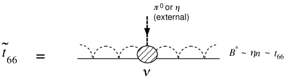
Figure 4: A diagram for the scattering amplitude of the meson($M$)-resonance($B^{*}$) coupling $\tilde{t}$. For $B^{*}\sim\eta n$, the relevant matrix element is $\tilde{t}_{66}$.

Figure 5: Diagrammatic representation for the vertex ${\cal V}$ of Fig. 4. Although the diagram (c) is disconnected, after the inclusion of rescattering terms of $t_{66}$, it will become connected as shown in Fig. 6(c)

Figure 6: Vertex functions of $\tilde{t}_{66}$ to lowest order in the rescattering. They are obtained by attaching $t_{66}$ in the lowest order to the elementary diagrams given in Fig. 5.

Now by attaching $t_{66}$ to the left and right of ${\cal V}$, we obtain $\tilde{t}_{66}$. First we consider the loop structure of $\tilde{t}_{66}$. The corresponding lowest order diagrams are shown in Figs. 6(a), (b) and (c). There are new types of loop integrals. We can, however, simplify and relate them to that of the meson baryon propagator $G_{l}$ of eq. (10) as follows:

Fig. 6(a)

Given the structure of the three meson vertices which are factorized out from the integral, each loop integral of Fig. 6(a) reduces to that of the meson-baryon propagator $G_{l}$.

Fig. 6(b)

The loop integrals here look new as they contain two meson propagators and one baryon propagator. However, the amplitudes of the diagrams (a) and (b) can combine in a way that one of the intermediate meson propagators of the diagram (b) cancels with part of the numerator coming from the $MM\rightarrow MM$ amplitude yielding the same loop as $G_{l}$. This will be explained in Fig. 8.

Fig. 6(c)

This diagram also looks new as it contains two baryon propagators and one meson propagator. Yet, we can show that in the case of static probe mesons, which we will adopt here, this loop can be derived from $G_{l}$ by differentiating with respect to a kinematical variable, similarly to what is done in quantum electrodynamics to derive the Ward identities.

3.2 $BBM$ vertex

In order to proceed, we investigate the structure of various vertices depicted in Figs. 5 and 6 in more detail. The simplest are the vertices of the Yukawa type ($BB^{\prime}M$) coupling. They are easily derived from the $D$ and $F$ terms of eq. (1) expanding $U$ up to one meson field. We find in a nonrelativistic reduction of the $\gamma^{\mu}\gamma^{5}$ matrix

$$-it_{B^{\prime}BM}=A_{B^{\prime}BM}\vec{\sigma}\cdot\vec{q}\,^{\prime}\,,$$ (20)

with

$$A_{B^{\prime}BM}=\left(x_{B^{\prime}BM}\frac{D+F}{2f}+y_{B^{\prime}BM}\frac{D-F}{2f}\right)\,,$$ (21)

where $\vec{q}\,^{\prime}$ refers to the momentum of the incoming probe meson $M$. The coefficients $x_{B^{\prime}BM}$ and $y_{B^{\prime}BM}$ are given in Table 2 for diagonal components. We need only diagonal matrix elements in the baryons, except for the possible case of $\Sigma^{0}\Lambda\pi^{0}$ in which $x_{\Sigma^{0}\Lambda\pi^{0}}=\frac{1}{\sqrt{3}}$ and $y_{\Sigma^{0}\Lambda\pi^{0}}=\frac{1}{\sqrt{3}}$. We shall also use in eq. (22) the $f$ corresponding to the meson which couple to the baryon, $f_{\pi}$ or $f_{\eta}$.

Table 2: Diagonal coefficients $x_{B^{\prime}BM}$ and $y_{B^{\prime}BM}$ of eq. (21).

. $\Sigma^{-}$ $\Sigma^{0}$ $\Lambda$ $p$ $n$ $x_{BB\pi^{0}}$ $-1$ 0 0 1 $-1$ $y_{BB\pi^{0}}$ 1 0 0 0 0 $x_{BB\eta}$ $\frac{1}{\sqrt{3}}$ $\frac{1}{\sqrt{3}}$ $-\frac{1}{\sqrt{3}}$ $\frac{1}{\sqrt{3}}$ $\frac{1}{\sqrt{3}}$ $y_{BB\eta}$ $\frac{1}{\sqrt{3}}$ $\frac{1}{\sqrt{3}}$ $-\frac{1}{\sqrt{3}}$ $-\frac{2}{\sqrt{3}}$ $-\frac{2}{\sqrt{3}}$

3.3 $BBMMM$ vertex

This vertex appears in the diagrams depicted in Figs. 5(a) and 6(a). The Lagrangians for the three meson–baryon vertices are obtained expanding $u_{\mu}$ in the $F$, $D$ terms of eq. (1) up to three meson fields. We obtain

$$u_{\mu}=\frac{\sqrt{2}}{12f^{3}}(\partial_{\mu}\Phi\Phi^{2}-2\Phi\partial_{\mu}\Phi\Phi+\Phi^{2}\partial_{\mu}\Phi)\,.$$ (22)

Expressions for the matrix elements of $u_{\mu}$ involving only nucleons were obtained in Ref. [24]. Here we have to generalize it for the case of hyperons also. Once again, by taking the nonrelativistic approximation of the $\gamma$ matrices, $\gamma^{\mu}\gamma^{5}\rightarrow\sigma^{i}$, we obtain

$$-it_{\alpha^{\prime}\alpha M}=C_{\alpha^{\prime}\alpha M}\vec{\sigma}\cdot\vec{q}\,^{\prime}\,,$$ (23)

with

$$C_{\alpha^{\prime}\alpha M}=\frac{1}{12f^{2}}\left(X_{\alpha^{\prime}\alpha M}\frac{D+F}{2f}+Y_{\alpha^{\prime}\alpha M}\frac{D-F}{2f}\right)\,,$$ (24)

where the coefficients, $X_{\alpha^{\prime}\alpha M}$, $Y_{\alpha^{\prime}\alpha M}$, with $\alpha$, $\alpha\,^{\prime}$ indicating a $MB$ state, are given in Tables 3 and 4 for $M\equiv{\pi}^{0}$, $\eta$ respectively. Once again the $f$ inside the brackets refers to $\pi$ or $\eta$, while the $f^{2}$ in the factor $12f^{2}$ will become $f_{\alpha}$ $f_{\alpha^{\prime}}$.

Table 3: $X_{lm}$ and $Y_{lm}$ coefficients for the three meson vertex, eq. (25) for $\pi^{0}$ coupling. They are symmetric as $X_{lm}=X_{ml}$ and $Y_{lm}=Y_{ml}$.

	$X_{lm}$						$Y_{lm}$
	$K^{+}\Sigma^{-}$	$K^{0}\Sigma^{0}$	$K^{0}\Lambda$	$\pi^{-}p$	$\pi^{0}n$	$\eta n$	$K^{+}\Sigma^{-}$	$K^{0}\Sigma^{0}$	$K^{0}\Lambda$	$\pi^{-}p$	$\pi^{0}n$	$\eta n$
$K^{+}\Sigma^{-}$	0	0	0	0	0	0	$-2$	0	0	0	$\frac{1}{\sqrt{2}}$	$\sqrt{\frac{3}{2}}$
$K^{0}\Sigma^{0}$		1	$-\frac{1}{\sqrt{3}}$	0	0	0		1	$-\frac{1}{\sqrt{3}}$	$-\frac{3}{\sqrt{2}}$	$-\frac{1}{2}$	$\frac{\sqrt{3}}{2}$
$K^{0}\Lambda$			$-1$	$\sqrt{6}$	$-\frac{1}{\sqrt{3}}$	1			$-1$	$-\sqrt{\frac{3}{2}}$	$\frac{1}{2\sqrt{3}}$	$-\frac{1}{2}$
$\pi^{-}p$				$-4$	$2\sqrt{2}$	0				0	0	0
$\pi^{0}n$					0	0					0	0
$\eta n$						0						0

Table 4: $X_{lm}$ and $Y_{lm}$ coefficients for the three meson vertex, eq. (25) for $\eta$ coupling. They are symmetric as $X_{lm}=X_{ml}$ and $Y_{lm}=Y_{ml}$.

	$X_{lm}$						$Y_{lm}$
	$K^{+}\Sigma^{-}$	$K^{0}\Sigma^{0}$	$K^{0}\Lambda$	$\pi^{-}p$	$\pi^{0}n$	$\eta n$	$K^{+}\Sigma^{-}$	$K^{0}\Sigma^{0}$	$K^{0}\Lambda$	$\pi^{-}p$	$\pi^{0}n$	$\eta n$
$K^{+}\Sigma^{-}$	0	$-\sqrt{3}$	$-1$	0	0	0	$-2\sqrt{3}$	$\sqrt{3}$	$-1$	0	$\sqrt{\frac{3}{2}}$	$\frac{3}{\sqrt{2}}$
$K^{0}\Sigma^{0}$		$-\sqrt{3}$	1	0	0	0		$-\sqrt{3}$	1	$\sqrt{\frac{3}{2}}$	$\frac{\sqrt{3}}{2}$	$-\frac{3}{2}$
$K^{0}\Lambda$			$\sqrt{3}$	$-\sqrt{2}$	1	$-\sqrt{3}$			$\sqrt{3}$	$\frac{1}{\sqrt{2}}$	$-\frac{1}{2}$	$\frac{\sqrt{3}}{2}$
$\pi^{-}p$				0	0	0				0	0	0
$\pi^{0}n$					0	0					0	0
$\eta n$						0						0

In eqs. (23) and (24), we have kept only the terms which survive when $t_{66}$ is attached to both sides of the three meson vertex, since the $N^{*}$ state should be dynamically generated by the scattering of the meson. Note that the successive $BBMM$-vertices $V_{ij}$, where the incoming or outgoing meson is scattered, are $s$-wave couplings. Due to this $s$-wave nature, the terms in eq. (22) which involve the derivatives acting on the two internal mesons vanish in the loop integral and only the term which has the derivative in the external $\pi^{0}$ or $\eta$ field survives.

3.4 $MMMM$ vertex

Finally we consider the terms involving the meson meson interaction which appear in Figs. 5(b) and 6(b). The evaluation of the $M_{1}M_{2}\rightarrow M_{1}^{\prime}M_{2}^{\prime}$ vertices has been done in Ref. [9]. Here we need in addition the meson propagator and a $B^{\prime}BM$ vertex in order to evaluate the diagrams of Fig. 6(b) and the related ones obtained by iterating to the right and left the meson baryon scattering potential, $V_{ij}$. Let us look in detail at these diagrams in some cases in order to see their general behavior.

Figure 7: The case involving the $\pi\pi\rightarrow\pi\pi$ vertex.

First let us take the case involving the $\pi\pi\rightarrow\pi\pi$ vertex as shown in Fig. 7. The contribution of this diagram is:

$$-it=(-i)\,t_{\pi^{-}\pi^{0}\rightarrow\pi^{-}\pi^{0}}\,\frac{i}{q^{2}-m_{\pi}^{2}}\,\frac{D+F}{2f}\,\vec{\sigma}\cdot{\vec{q}}\,,$$ (25)

where

$$t_{\pi^{-}\pi^{0}\rightarrow\pi^{-}\pi^{0}}=-\frac{1}{3f^{2}}[3(k_{1}-k_{2})^{2}-\sum p_{i}^{2}+m_{\pi}^{2}]\,.$$ (26)

We note that the $\pi^{-}\pi^{0}\rightarrow\pi^{-}\pi^{0}$ vertex function has an off shell behavior since it involves $\sum{p_{i}^{2}}$ where $p_{i}$ is the momentum of each of the pion lines. The first step is to recall that, following the steps of Ref. [9], the $MM$ amplitude in the loops has to be taken with $p_{i}^{2}=m_{i}^{2}$, since the terms with $p_{i}^{2}-m_{i}^{2}$ will kill one of the off shell propagators and renormalize other diagrams already considered. This is illustrated in Fig. 8, where starting from diagram (a), the term $k_{1}^{2}-m_{\pi}^{2}$ would eliminate the internal meson propagator of momentum $k_{1}$ and lead to diagram (b), which can be interpreted as a vertex correction of the three pion vertex, i.e., the diagram (a) of Fig. 5, as shown in the diagram Fig. 8(c). This can be reabsorbed into the physical coupling of the vertex of Fig. 5(a).

Figure 8: Diagram obtained from the diagram of Fig. 6(b) when the off shell part of the meson meson amplitude is considered.

Next we consider the first term of eq. (26)

$$(k_{1}-k_{2})^{2}=(q-q^{\prime})^{2}\,.$$ (27)

In order to have the same kinematics of the $N^{\ast}$ to the right and left of the $\pi^{0}N^{\ast}N^{\ast}$ vertex we shall take $q^{\prime\,{\mu}}\rightarrow 0$ (soft pion limit). We are concerned about the coefficient which will accompany $\vec{\sigma}\cdot\vec{q}\,^{\prime}$ for this vertex and this coefficient will be roughly independent of $q^{\prime}$ as is the case of the $\pi NN$ vertex in the nonrelativistic limit that we take. Hence

$$(k_{1}-k_{2})^{2}\simeq q^{2}$$ (28)

in this limit. Keeping the other terms in eq. (27) would lead to $q^{2}+m_{\pi}^{2}$ since the linear term in $q$ would vanish in the loops. The limit taken neglects $m_{\pi}^{2}$ versus $q^{2}$ which is certainly a fair approximation. Consistency with that approximation will require the neglect of the terms proportional to $m_{\pi}^{2}$ when they appear and we shall do so in the evaluations here.

On the other hand the term $\vec{\sigma}\cdot\vec{q}$ in eq. (25) can be rewritten as:

$$\vec{\sigma}\cdot\vec{q}=\vec{\sigma}\cdot(\vec{k}_{1}+\vec{q}\,^{\prime}-\vec{k}_{2})$$ (29)

and the terms proportional to $\vec{k}_{1}$, $\vec{k}_{2}$ will vanish in the loops. Hence we can write the contribution of the diagram of Fig. 7 in an effective way as:

$$-it=-\frac{1}{f^{2}}\,(q^{2}-m_{\pi}^{2})\,\frac{1}{q^{2}-m_{\pi}^{2}}\,\frac{D+F}{2f}\vec{\sigma}\cdot{\vec{q}\,^{\prime}}\,.$$ (30)

In this equation we see that the meson propagator cancels with the remnant of the $\pi\pi\rightarrow\pi\pi$ vertex and we obtain a structure of the type of the three meson vertex of Fig. 6(a). Chiral symmetry brings always these two kind of diagrams together as is well known from early studies of $\pi N\rightarrow\pi\pi N$ interaction [25] prior to the more systematic $\chi PT$ approach to these amplitudes. The result obtained indicates that the contribution of these terms can be cast in the same way as in eq. (24).

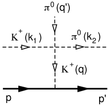
Figure 9: Feynman diagram for the $K^{+}\pi^{0}\rightarrow K^{+}\pi^{0}$ vertex.

Let us see another example shown in Fig. 9. In this case the $K^{+}\pi^{0}\rightarrow K^{+}\pi^{0}$ vertex, which we take from the $K^{+}K^{-}\rightarrow\pi^{0}\pi^{0}$ amplitude of Ref. [9] via crossing, can be written after setting $p_{i}^{2}=m_{i}^{2}$ as:

$$-\frac{3}{4f^{2}}t=-\frac{3}{4f^{2}}(k_{1}-q)^{2}=-\frac{3}{4f^{2}}(k_{2}-q^{\prime})^{2}\simeq-\frac{3}{4f^{2}}k_{2}^{2}\,,$$ (31)

and the on shell condition will rend this as a term proportional to $m_{\pi}^{2}$ which we will neglect. Note that in addition we would have one loop with two heavy meson propagators which would further reduce the strength of the diagram.

The argument above would lead to a term proportional to $m_{\eta}^{2}$ if the $\pi^{0}$ with momentum $k_{2}$ is substituted by an $\eta$. This term would not be small in principle. However, the $K^{+}$ attached to the baryon would involve the $K^{+}\Sigma^{-}n$ vertex which goes like ($F-D$), small compared to the $F+D$ component. Furthermore it would contain two loops involving each two heavy mesons which would further reduce the contribution.

The arguments used above have been used in order to justify that terms of the type of Fig. 9 with a heavy meson exchange attached to the baryon line, with one loop to the right and another one to the left, should be small compared to those where just a pion is attached to the baryon line. We will just adopt this approximation and keep only the terms where a pion is exchanged there. Under these approximations the diagrams of the type of Figs. 7 and 9 can be cast in terms of an effective operator similar to eq. (24) as:

$$-it_{\alpha^{\prime}\alpha M}=\tilde{C}_{\alpha^{\prime}\alpha M}\vec{\sigma}\cdot{\vec{q}\,^{\prime}}\,,$$ (32)

where

$$\tilde{C}_{\alpha^{\prime}\alpha M}=\frac{1}{12f^{2}}\left(\tilde{X}_{\alpha^{\prime}\alpha M}\frac{D+F}{2f}+\tilde{Y}_{\alpha^{\prime}\alpha M}\frac{D-F}{2f}\right)\,,$$ (33)

and the $\tilde{X}$ and $\tilde{Y}$ coefficients are given in Table 5 for an external $\pi^{0}$ coupling. The same comments given after eq. (25) concerning the values of the $f^{\prime}s$ are in order here. For the case of $\eta$ external coupling and intermediate $\pi$ attached to the baryon line, the $MM\rightarrow MM$ vertices with three pions and one $\eta$ are either zero or proportional to $m_{\pi}^{2}$, which we omit in our analysis. Surviving terms would involve loops with two kaons and $\Sigma$ or $\Lambda$ which should be suppressed. We will omit these terms and then within this approximation the $\tilde{X}$, $\tilde{Y}$ coefficients for the external $\eta$ will be taken zero. In the case of the $\eta$ the soft meson limit is also a drastic approximation. Altogether this means that for the $\eta N^{\ast}N^{\ast}$ coupling we should admit larger uncertainties than for the $\pi^{0}N^{\ast}N^{\ast}$ coupling, where the approximations done are rather sensible.

Table 5: $\tilde{X}_{lm}$ and $\tilde{Y}_{lm}$ coefficients of eq. (34). They are symmetric as $\tilde{X}_{lm}=\tilde{X}_{ml}$ and $\tilde{Y}_{lm}=\tilde{Y}_{ml}$.

	$\tilde{X}_{lm}$						$\tilde{Y}_{lm}$
	$K^{+}\Sigma^{-}$	$K^{0}\Sigma^{0}$	$K^{0}\Lambda$	$\pi^{-}p$	$\pi^{0}n$	$\eta n$	$K^{+}\Sigma^{-}$	$K^{0}\Sigma^{0}$	$K^{0}\Lambda$	$\pi^{-}p$	$\pi^{0}n$	$\eta n$
$K^{+}\Sigma^{-}$	3	0	0	0	0	$0$	$-3$	0	0	0	0	$0$
$K^{0}\Sigma^{0}$		0	$-\sqrt{3}$	0	0	0		0	$-\sqrt{3}$	0	0	0
$K^{0}\Lambda$			0	0	0	$0$			0	0	0	0
$\pi^{-}p$				$-12$	0	0				0	0	0
$\pi^{0}n$					0	0					0	0
$\eta n$						0						0

To end this subsection, we note that in diagrams (a), (b) of Fig. 6 we can sum the two contributions of the type of Fig. 5 (a), (b) in one block by means of

$$-t_{\alpha^{\prime}\alpha^{\prime}M}=D_{\alpha^{\prime}\alpha M}\vec{\sigma}\cdot\vec{q}\,^{\prime}\,,$$ (34)

with

$$D_{\alpha^{\prime}\alpha M}=\frac{1}{12f^{2}}\left((X_{\alpha^{\prime}\alpha M}+\tilde{X}_{\alpha^{\prime}\alpha M})\frac{D+F}{2f}+(Y_{\alpha^{\prime}\alpha M}+\tilde{Y}_{\alpha^{\prime}\alpha M})\frac{D-F}{2f}\right)\ ,$$ (35)

with the same considerations about the $f$ factors as given after eq. (25).

4 Generation of the $\pi^{0}(\eta)N^{\ast}N^{\ast}$ vertex.

From the series of Fig. 4 we must pick up the terms which factorize the $\eta n$ amplitude to the left and the right of the external $\pi^{0}(\eta)$ vertex since this amplitude contains the $N^{\ast}$ pole and hence the resulting amplitude can be compared to the conventional one which appears from the diagram of Fig. 10.

Figure 10: Diagrammatic representation of the $\pi N^{\ast}N^{\ast}$ couplings with explicit $N^{\ast}$ propagators.

Hence we shall start from $\eta n$ in the series of Fig. 4 and finish up with $\eta n$ for simplicity. The resulting amplitude will be compared to the one of Fig. 10 which is given by (the index 6 stands for the 6th channel of $\eta n$ in Table 1)

$$-i\tilde{t}_{66}(\sqrt{s})=(-ig_{\eta})\frac{i}{\sqrt{s}-M^{\ast}+i\frac{\Gamma(s)}{2}}\,C\,\vec{\sigma}\cdot\vec{q}\,^{\prime}\frac{i}{\sqrt{s}-M^{\ast}+i\frac{\Gamma(s)}{2}}\,(-ig_{\eta})\,,$$ (36)

where $C\vec{\sigma}\cdot\vec{q}\,^{\prime}$ is the $N^{\ast}N^{\ast}\pi^{0}$ coupling, to be compared with $-(D+F)\vec{\sigma}\cdot\vec{q}\,^{\prime}/2f$ of $\pi^{0}nn$ in the case of nucleons. On the other hand the $\eta n\rightarrow\eta n$ amplitude proceeding through $N^{\ast}$ excitation is depicted in Fig. 11 and given by

$$-it_{66}(\sqrt{s})=(-ig_{\eta})\frac{i}{\sqrt{s}-M^{\ast}+i\frac{\Gamma(s)}{2}}(-ig_{\eta})\,.$$ (37)

Figure 11: Diagrammatic representation of the $\eta n\rightarrow\eta n$ process through explicit $N^{\ast}$ excitation.

Our aim is to evaluate the coupling constant $C$ in eq. (36). This will be accomplished by dividing the amplitude by $g_{\eta}^{2}$ and the square of the $N^{\ast}$ propagator. We should note that the fact that the $\eta N$ threshold (1486 MeV) is below the $N^{\ast}$ mass (1550 MeV) makes the width $\Gamma$ in eqs. (36) and (37) strongly energy dependent, particularly close to the $\eta N$ threshold. Hence $t_{66}$ in eq. (37) differs from a Breit Wigner distribution close to the $\eta N$ threshold but resembles it much better at energies above the $N^{\ast}$ mass. This situation is shown in Figs. 12 (a)-(d), where the $t_{66}(\eta n\to\eta n)$ and $t_{46}(\pi^{-}p\to\eta n)$ amplitudes of (a) and (b) are compared with the Breit-Wigner amplitudes of (c) and (d).

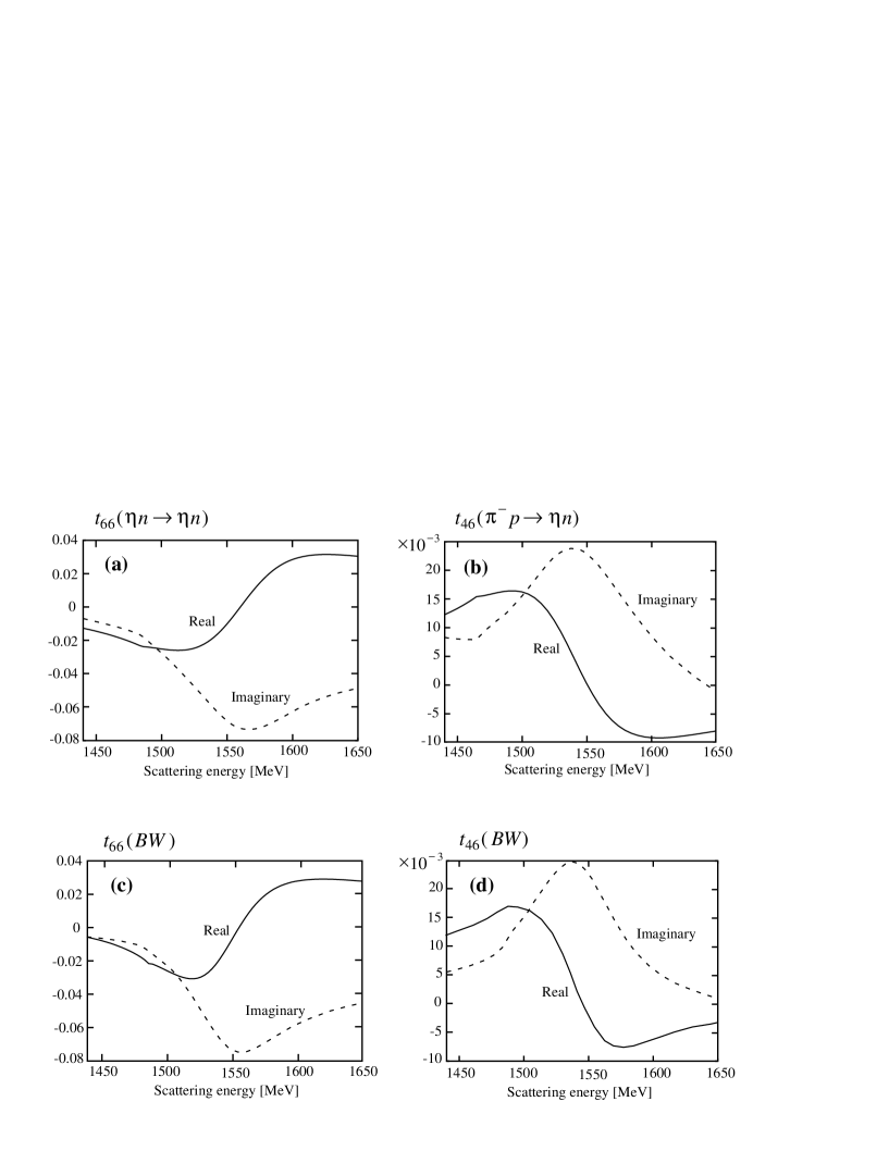
Figure 12: Real and imaginary parts of the $t_{66}(\eta n\to\eta n)$ (a), $t_{46}(\pi^{-}p\to\eta n)$ (b) and the corresponding Breit-Wigner amplitudes suplemented by the background ((c) and (d) for eqs. (14) and (15)) as functions of the scattering energy $\sqrt{s}$.

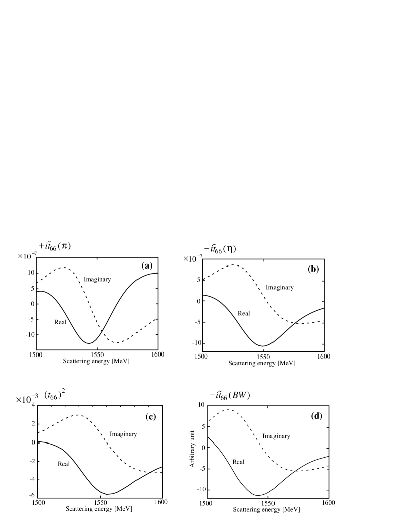
Figure 13: Comparison of the amplitude $i\tilde{t}_{66}$ for the pion coupling (a) and $-i\tilde{t}_{66}$ for the eta coupling (b), where the factor $\vec{\sigma}\cdot\vec{q}\,^{\prime}$ has been removed, with $t_{66}^{2}$ (c), as functions of the scattering energy $\sqrt{s}$. The amplitude $-i\tilde{t}_{66}(BW)$, obtained assuming a Breit Wigner form for $t_{66}$ (eq. (37)), is also shown ((d) in arbitrary units).

The amplitude $\tilde{t}_{66}$ both for an external $\pi^{0}$ and $\eta^{0}$ behaves approximately as the square of a Breit Wigner distribution. Indeed, one should note that all the matrices $t_{6l}$ contain the $N^{\ast}$ pole. This can be seen from eq. (8) which reads in matrix form

$$t=[1-VG]^{-1}V$$ (38)

and all matrix elements have a pole where det$[1-VG]$ = 0, which occurs in the second Riemann sheet of the complex plane and corresponds to the $N^{\ast}$ pole. Hence $\tilde{t}_{66}$ should contain the $N^{\ast}$ propagator squared as implied by eq. (36). In the vicinity of the complex pole, the $N^{*}$ propagator becomes infinite and the $N^{*}$ contribution dominates the process. However, if we move on the real axis for the energy, hence slightly apart from the pole, the background in the amplitudes can be nonnegligible, as we found in eqs. (12-13), and the $6\times 6$ amplitudes which can be generated with the 6 states of Table 1 have slightly different shapes around the $N^{\ast}$ energy causing the peak of $|{\rm Im}\,\tilde{t}|$ to fluctuate around the $N^{\ast}$ mass. As a consequence, the shapes of $\tilde{t}_{66}$ for an external pion or eta are slightly different and also different from $t_{66}^{2}$, although all of them are qualitatively similar as can be seen in Fig. 13. For these reasons, the Breit Wigner shape is better realized to the right of the peak. Therefore, it is better to compare ${\rm Re}\,(-i\tilde{t}_{66})$ with ${\rm Re}\,(t^{2}_{66})$ at the point where they have their maximum strength to the right of the resonance, which happens to be close to the $M^{\ast}$ pole. In this way we avoid improper comparisons due to the small shifts in the apparent peak position of the different channels. In doing so we minimize the effect of the background since ${\rm Re}\,(t_{66}^{2})$ at its peak comes mostly from (${\rm Im}\,\,t_{66})^{2}$. However, considering that the background could account for $15\%$ of ${\rm Im}\,\,t$ at its peak, we should accept uncertainties of the order of $30\%$ in the results from this kind of analysis. Hence we take

$$C\vec{\sigma}\cdot\vec{q}^{\;\prime}\simeq g_{\eta}^{2}\frac{{\rm Re}\,(-i\tilde{t}_{66})}{{\rm Re}\,(t_{66}^{2})}.$$ (39)

Our technical procedure will be to evaluate $\tilde{t}_{66}$ from the series of Fig. 6 and apply eq. (40), using the amplitude ${t}_{66}$ provided by the model of section 2. It is not difficult to see that the $\tilde{t}_{66}$ amplitude for an external $\pi^{0}$ is evaluated by

$$-i\tilde{t}_{66} = \sum_{l,m}t_{6l}\,G_{l}\,D_{lm\pi^{0}}\,\vec{\sigma}\cdot\ \vec{q}\,^{\prime}G_{m}\,t_{m6}+\sum_{l}t_{6l}\,\tilde{G_{l}}\,A_{l}\,\vec{\sigma}\cdot\vec{q}\,^{\prime}t_{l6}$$ (40)

$$+ t_{62}\tilde{G}^{\ast}A_{\Sigma^{0}\Lambda\pi^{0}}\,\vec{\sigma}\cdot\vec{q}\,^{\prime}t_{36}+t_{63}\tilde{G}^{\ast}A_{\Sigma^{0}\Lambda\pi^{0}}\,\vec{\sigma}\cdot\vec{q}\,^{\prime}t_{26}\ ,$$

where

$$\tilde{G_{l}}=i\int\frac{d^{4}q}{(2\pi)^{4}}\frac{M_{l}}{E_{l}(\vec{q}\,)}\frac{M_{l}}{E_{l}(\vec{q}\,)}\left(\frac{1}{\sqrt{s}-q^{0}-E_{l}(\vec{q}\,)+i\epsilon}\right)^{2}\frac{1}{q^{2}-m_{l}^{2}+i\epsilon}\,.$$ (41)

Here by taking $q^{\prime\mu}\rightarrow 0$, the square of the baryon propagator appears. The coefficients $D_{lm\pi^{0}}$ in eq. (40) are given by eq. (35), and the coefficients $A_{l}$ are abbreviations for $A_{ll\pi^{0}}$, the diagonal $A_{B^{\prime}BM}$ coefficients of eq. (22). The last two terms in eq. (40) correspond to Fig. 6(c) with intermediate $\Sigma^{0}$, $\Lambda$ or $\Lambda$, $\Sigma^{0}$ respectively. For the meson baryon propagator $\tilde{G}^{\ast}$ we take here the same formula as eq. (41) averaged for the $\Lambda$ and the $\Sigma^{0}$. Since there is no $\Sigma^{0}\Lambda\eta$ coupling, these last two terms in eq. (40) do not appear for the case of the external $\eta$.

By taking one of the $M/E$ factors unity, we can obtain $\tilde{G}_{l}$ from $G_{l}$ by differentiating with respect to $\sqrt{s}$

$$\tilde{G}_{l}=-\frac{\partial{G_{l}}}{\partial\sqrt{s}}\ .$$ (42)

We note that eq.(42) presents a singularity at the meson-baryon threshold, which disappears if $q^{\prime\,\mu}\neq 0$ because the square of the baryon propagator is replaced by the product of two different propagators. This singularity fades away rapidly as one moves away from threshold, as one can see in Fig. 13 where for $\sqrt{s}>1500$ MeV, only 14 MeV above the $\eta N$ threshold, there is already no sign of the singular behavior. It is clear that in this procedure there is some element of arbitrariness because in order to evaluate $G_{l}$ we have fixed the cut off arbitrarily and adjusted the $a_{l}$ coefficients to the data. Since $a_{l}$ is a constant it will not contribute in the derivative of eq. (42). In order to estimate the uncertainties from this procedure we conduct a test consisting in increasing and decreasing the cut off by about 30 % to 1300 MeV and 700 MeV respectively. Accordingly the $a_{l}$ coefficients of eq. (10) are changed such that at the energy of the $N^{*}$ resonance $G_{l}$ takes the same value. However, $\tilde{G}_{l}$ would now change and so the results for $C$. When we conduct this test we find that the amplitudes in Figs. 12 and 13 are barely changed. The changes are of the order of 5 % . This gives us confidence about the fairness of the method used to evaluate the couplings.

5 Results and discussions

5.1 Numerical results

As we explained in section 3, we consider the zero charge state for $N^{\ast}(1535)$. The evaluation of the $C$ coefficient for $\pi^{0}N^{\ast}N^{\ast}$ gives us:

$$C_{\pi^{0}N^{\ast}N^{\ast}}=-7.09\cdot 10^{-4}\;{\rm MeV}^{-1}\;,$$ (43)

with an admitted uncertainty of around 30 $\%$.

The number $C$ in eq. (44) should be compared with the equivalent coupling $\pi^{0}NN$, which is given by $-\displaystyle\frac{D+F}{2f}$ with $D+F=1.26=g_{A}$. Hence we find

$$\frac{C_{\pi^{0}N^{\ast}N^{\ast}}}{C_{\pi^{0}NN}}\sim 0.11\,,$$ (44)

which tells us that the $\pi N^{\ast}N^{\ast}$ coupling of about $10\%$ of the $\pi NN$ one and has equal sign. We have checked that the sign is stable under changes of the parameters compatible with the data. Hence this would rule out the possibility of the mirror assignment. Using the ratio of the Goldberger-Treiman relations for $N$ and $N^{\ast}$

$$g_{A}^{*}=\frac{M}{M^{*}}\frac{C_{\pi^{0}N^{\ast}N^{\ast}}}{C_{\pi^{0}NN}}g_{A}\,,$$ (45)

one can relate the number in eq. (44) to $g_{A}^{*}$:

$$g_{A}^{*}\sim 0.08\,.$$ (46)

As for the $\eta$ coupling we obtain:

$$C_{\eta N^{\ast}N^{\ast}}=5.83\cdot 10^{-4}\;{\rm MeV}^{-1}\ .$$ (47)

This gives the ratio:

$$\frac{C_{\eta N^{\ast}N^{\ast}}}{C_{\pi^{0}NN}}=0.09\,.$$ (48)

The strength of the $\eta$ coupling here is less than $10\%$ of that of the pion. Here, in addition to the $30\%$ uncertainties due to the non resonant background we should consider additional ones as we have discussed above.

In order to have some feeling for the strength of the different terms we summarize here the general trends of the numerics.

1. For the case of the pion coupling the contribution of the first term in eq. (41), the $GDG$ term, is about one order of magnitude smaller than the terms involving $\tilde{G}$. The sum of the two terms in eq. (41) involving the $\tilde{G^{\ast}}$ are smaller than the one involving $\tilde{G}$ but of the same order of magnitude.

2. Given the dominance of the $\tilde{G}$ terms, we find a cancellation between the terms $\pi^{-}p$ and $\pi^{0}n$ intermediate states (because of the isospin factor in $\pi NN$, see Table 2) and hence the contribution is dominated by the $\eta n$ and $K^{+}\Sigma^{-}$ intermediate states between which there is still some partial cancellation.

3. For the case of the eta coupling the contribution of the $\tilde{G}$ terms is also dominant over the $GDG$ combination, and as we mentioned, the last two terms in eq. (41) do not appear in this case. Furthermore, there is no cancellation between the pion intermediate states (because of the isospin of the $\eta$, see Table 2). The dominant terms come from the $K\Sigma$ and $K\Lambda$ intermediate states in which there are some partial cancellations.

5.2 Comparison with quark models

It would be interesting to compare the present result with other model calculations. There are several examples which appear to support the present result.

First we discuss the implications of the nonrelativistic (NR) quark model, where the negative parity baryons emerge as orbitally excited states of $l=1$ ($p$ state). There are two independent states for $1/2^{-}$:

$$|1\rangle = [l=1,S=1/2]^{1/2^{-}}\,,$$

$$|2\rangle = [l=1,S=3/2]^{1/2^{-}}\,,$$ (49)

where the $p$ state is coupled either by the total spin $S=1/2$ state or $S=3/2$. In the presence of a tensor force, these two states are mixed and their linear combinations are interpreted as physical resonances:

$$|N^{*}(1535)\rangle = a|1\rangle-b|2\rangle\,,$$ (50)

$$|N^{*}(1650)\rangle = b|1\rangle+a|2\rangle\,.$$ (51)

Here the coefficients $a$ and $b$ are real and satisfy $a^{2}+b^{2}=1$ ($b>0$).

The axial vector coupling constant is then defined by

$$g^{*}_{A}=\langle p^{*}(1535),s_{z}=1/2|\sum_{i=1,2,3}\sigma_{3}^{(i)}\tau_{3}^{(i)}|p^{*}(1535),s_{z}=1/2\rangle\,,$$ (52)

where $\sigma^{(i)}$ and $\tau^{(i)}$ are quark spin and isospin matrices for the $i$-th quark and the sum runs over the three quarks. The matrix element of eq. (53) is easily computed and the result is

$$g^{*}_{A}=\frac{1}{9}\left(-a^{2}+16a\sqrt{1-a^{2}}+5(1-a^{2})\right)\,.$$ (53)

In Fig. 14 we show $g^{*}_{A}$ as a function of the mixing coefficient $a$. We see that depending on the value of $a$, the coupling constant $g^{*}_{A}$ can be either positive or negative. In the successful model by Isgur and Karl [26], the mixing coefficient takes the value $a\sim 0.85$, yielding an axial vector coupling constant $g^{*}_{A}\sim 0.87$, which is about an order of magnitude larger than the present results. One should also note, from input of Fig. 14, that a slight increase of the mixing coefficient above the value 0.85 would reduce drastically $g_{A}^{\ast}$.

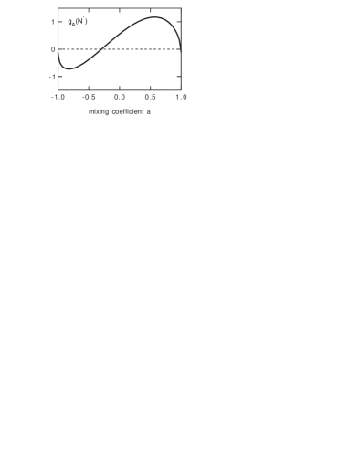
Figure 14: $g_{A}^{\ast}$ as a function of the mixing coefficient $a$.

Another interesting case is presented by the large-$N_{c}$ consideration. A somewhat nontrivial assumption here is the hedgehog correlation, where spin and isospin degrees of freedom are strongly correlated such that the intrinsic state acquire the grand spin $\vec{K}=\vec{J}+\vec{I}=0$. Here $J$ is the total spin, $\vec{J}=\vec{L}+\vec{S}$, and $\vec{I}$ the isospin. In the large-$N_{c}$ limit, quark-quark interactions become small as the Hartree approximation becomes exact. Hence the hedgehog configuration is assumed for each quark separately. For $s$ and $p$ quarks, such hedgehog states are

$$|h\rangle = [s,\tau]^{K}=[1/2,\,1/2]^{0}\,,$$ (54)

$$|h^{*}\rangle = [[l,s]^{j},\tau]^{K}=[[1,1/2]^{1/2},\,1/2]^{0}\,.$$ (55)

Hence the negative parity hedgehog for $N^{*}(1535)$ in the large-$N_{c}$ limit takes the form

$$|H\rangle=\frac{1}{N_{c}}\left(|h^{*}\,h\cdots h\rangle+\cdots|h\cdots h,h^{*}\rangle\right)\,.$$ (56)

Physical baryon states are projected out from the hedgehog state by applying the projection operator:

$$|B\rangle\sim\int d[\omega]\,D^{*}_{B}(\omega)\,R^{\tau}(\omega)\,|H\rangle\,,$$ (57)

where $R^{\tau}(\omega)$ is the rotation operator in isospin space and $D^{*}_{B}(\omega)$ the $D$-function for a physical baryon state $B$.

For $N_{c}=3$ the integral in eq. (57) yields

$$|B=1/2^{-}\rangle=\frac{1}{\sqrt{2}}(|1\rangle-|2\rangle)\,,$$ (58)

where the states $|1\rangle$ and $|2\rangle$ are those given in eqs. (49). Thus the mixing coefficient $a$ in this case is precisely $1/\sqrt{2}$ and the corresponding $g_{A}^{*}=1.11$. We note that this mixing rate is consistent with the result obtained in a phenomenological analysis based on the large-$N_{c}$ [27].

From these considerations, our present results look very much different from the quark model results. The discrepancy, however, should not be a big surprise since the $N^{\ast}(1535)$ as well the $\Lambda(1405)$ resonances are cases known to be somewhat pathological within standard quark models. Actually we are giving a rather different interpretation of this resonance as a kind of quasibound meson baryon state in coupled channels. However, it is also worth noting that other versions of quark models which account for relativistic corrections in the $\pi qq$ coupling [28] lead to values of $C_{\pi^{0}N^{\ast}N^{\ast}}/C_{\pi^{0}NN}$ between 0.06 and 0.1, depending on the confining potential used, in agreement with our results of eq. (45).

6 Conclusions

We have evaluated the $N^{\ast}N^{\ast}\pi^{0}$ and $N^{\ast}N^{\ast}\eta$ couplings using a chiral unitary approach where the $N^{\ast}(1535)$ is generated dynamically. We could generate these couplings in terms of known couplings of the $\pi$, $\eta$ to baryons and other mesons as given by the chiral Lagrangians. The values obtained are about one order of magnitude smaller than the $\pi NN$ coupling. In the case of the $\pi N^{\ast}N^{\ast}$ coupling we get the same sign as the $\pi NN$ one. This is the sign expected for the naive assignment in the chiral doublet combining mesons and baryons. The uncertainties in the approach followed here can not reverse this sign, hence the present calculations appear to rule out the mirror case.

We have compared the present result with other models for $N^{*}$, e.g., the nonrelativistic quark model of Isgur-Karl, the large-$N_{c}$ approach and the relativised quark model of Cano et al. [28]. We have found that all of them predict values for $g_{\pi N^{\ast}N^{\ast}}$ and $g_{A}$ with the same sign. Hence, $N^{*}(1535)$ which appears as the first resonance state in the pion (and eta) scatterings is likely to carry a naive chiral assignment together with the ground state nucleon. However we find absolute values for $g_{\pi N^{\ast}N^{\ast}}$ coupling roughly one order of magnitude smaller than those of quark models, except the one of Cano et al., which has about the same order of magnitude.

It would be further interesting if we can confirm our theoretical implication in experiments. Since we can not have a stable target for $N^{*}(1535)$, the measurement of coupling constants will necessarily require somewhat complicated processes. One such candidate is to measure a two meson production of the pion and eta simultaneously [29]. The eta meson can be used as a probe for the production of $N^{*}(1535)$. Then, another pion can be produced either at the $N^{*}(1535)$ or at the nucleon with coupling constants $g_{\pi N^{*}N^{*}}$ and $g_{\pi NN}$, respectively, as illustrated in Fig. 15. Actually, there could be other diagrams which are not shown in Fig. 15. For instance, the contact term of $N^{*}\pi\eta N$ can be generated by the same method as done here by generating the resonance only to the left of the vertex. Before performing concrete calculations, however, we can expect that from a naive consideration of energy denominators as emphasized for example by Ochi et al [30], the diagrams shown in Fig. 15 are two of the dominant contributions from which we could extract information on the sign of the coupling through their interference effect. Depending on the sign of the two couplings, the two terms can be added either constructively or destructively. One may use such coherent processes to see the relative sign of the two coupling constants [13]. Even if only some bounds on the coupling could be obtained (in view of the smallness of our predictions) this would still be valuable information.

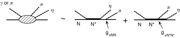
Figure 15: A resonance dominant process for the two meson production of $\pi$ and $\eta$.

The exercise done here has also served to show how one can technically implement the coupling of an external pion or eta to a resonance structure. These techniques can easily be generalized to obtain the coupling of other external sources as photons, vector mesons, etc, which would enable one to evaluate magnetic moments of resonances and other electromagnetic or weak properties.

Acknowledgments

We are grateful to the COE Professorship program of Monbusho, which enabled E. O. to stay at RCNP to perform the present work. Useful discussions and ideas from J. A. Oller are much appreciated. A.P. would like to acknowledge Prof. R.A. Arndt and N. Kaiser for providing her with some experimental data and other helpful information. A.H. and M.O thank D. Jido for discussions on $\pi$ and $\eta$ productions. J.C. Nacher would like to acknowledge the hospitality of the RCNP of the Osaka University where this work was done and support from the Ministerio de Educación y Cultura. This work is partly supported by DGICYT contract number PB96-0753 and PB98-1247, and also by DOE Grant DE-FG06-91ER40561.

References

- [1] S. Coleman, Aspects of Symmetry, Cambrige University Press, Cambrige (1985).
- [2] J. Gasser and H. Leutwyler, Nucl. Phys. B250 (1985) 465.
- [3] U. G. Meissner, Rep. Prog. Phys. 56 (1993) 903.
- [4] A. Pich, Rep. Prog. Phys. 58 (1995) 563.
- [5] G. Ecker, Prog. Part. Nucl. Phys. 35 (1995) 1.
- [6] V. Bernard, N. Kaiser and U. G. Meissner, Int. J. Mod. Phys. E4 (1995) 193.
- [7] J. A. Oller, E. Oset and J. R. Peláez, Phys. Rev. Lett. 80(1998)3452; Phys. Rev. D 59 (1999) 71001; erratum Phys. Rev. D60 (1999) 099906.
- [8] F. Guerrero and J. A. Oller, Nucl. Phys. B 537 (1999) 459.
- [9] J. A. Oller and E. Oset, Nucl. Phys. A620 (1997) 438; erratum Nucl. Phys. A 652 (1999) 407.
- [10] J. A. Oller and E. Oset, Phys. Rev. D60 (1999) 074023.
- [11] G. Ecker, J. Gasser, A. Pich and E. de Rafael, Nucl. Phys. B321 (1989) 311.
- [12] D. Jido, M. Oka and A. Hosaka, Physical Review Letters, 80 (1998) 448.
- [13] D. Jido, Y. Nemoto, M. Oka and A. Hosaka, TIT Preprint (1998), also hep-ph/9805306, to appear in Nucl. Phys. A.
- [14] H. Kim, D. Jido and M. Oka, Nucl. Phys. A640 (1998) 77.
- [15] N. Kaiser, P. B. Siegel and W. Weise, Phys. Lett. B 362 (1995) 23.
- [16] N. Kaiser, P. B. Siegel and W. Weise, Nucl. Phys. A594 (1995) 325.
- [17] N. Kaiser, T. Waas and W. Weise, Nucl. Phys. A612 (1997) 297.
- [18] E. Oset and A. Ramos, Nucl. Phys. A635 (1998) 99.
- [19] M. Roos, Phys. Lett. B246 (1990) 179.
- [20] L. Castillejo, R.H. Dalitz and F.J. Dyson, Phys. Rev. 101 (1956) 453.
- [21] J. Caro Ramon, N. Kaiser, S. Wetzel and W. Weise, nucl-th/9912035, to be published in Nucl. Phys. A.
- [22] Particle Data Group, C. Caso et al, Eur. Phys. Jour. C3(1998)1
- [23] H. C. Chiang, E. Oset and L. C. Liu, Phys. Rev. C44 (1991) 738
- [24] U. G. Meissner, E. Oset and A. Pich, Phys. Lett. B353 (1995) 161.
- [25] S. Weinberg, Phys. Rev. Lett. 18 (1967) 188.
- [26] N. Isgur and G. Karl, Phys. Lett. 72B (1977) 109; ibid. 74B (1978) 353; Phys. Rev. D18 (1978) 4187; ibid. D20 (1979) 1191
- [27] C.D. Carone, H. Georgi, L. Kaplan and D. Morin, Phys.Rev. D50 (1994) 5793.
- [28] F. Cano, P. González, B. Desplanques, S. Noguera, Z. Phys. A359 (1997) 315-319; F. Cano, P. González, S. Noguera, B. Desplanques, Nucl. Phys. A603 (1996) 257-280; F. Cano, private communication
- [29] D. Jido, M. Oka and A. Hosaka, in preparation.
- [30] K. Ochi, M. Hirata and T. Takaki, Phys. Rev. C56 (1997) 1472, and private communication from T. Takaki.