Nucleon-Nucleon Effective Field Theory at NNLO: Radiation Pions and ${}^{1}S_{0}$ Phase Shift

Low energy phenomena involving two nucleons can be successfully described using effective field theory. Because of the relatively large expansion parameter, it is only at next-to-next-to-leading order (NNLO) where one can expect to see agreement with experiment at the few percent level. The first part of this talk will focus on radiation pion effects, which first appear at NNLO. The power counting for radiation pions is simple for center of mass momentum $p\sim\sqrt{Mm_{\pi}}\equiv Q_{r}$, the threshold for pion production. We explain how graphs calculated with the $Q_{r}$ power counting scale for $p\sim m_{\pi}$. The $Q_{r}^{3}$ radiation pion contributions to nucleon-nucleon scattering are suppressed by inverse powers of the S-wave scattering lengths. However, we point out that order $Q_{r}^{4}$ radiation contributions might give a NNLO contribution for $p\sim m_{\pi}$. In the second part of the talk, results for the potential pion and contact interaction part of the NNLO ${}^{1}S_{0}$ phase shift are presented. We emphasize the importance of eliminating spurious poles in the expression for the amplitude at each order in the perturbative expansion. Doing this leaves a total of three free parameters at NNLO. We obtain a good fit to the ${}^{1}S_{0}$ phase shift.

Introduction

This talk focuses on higher order calculations in the low energy effective field theory for two-nucleon systems. In particular, we will be discussing nucleon-nucleon scattering at next-to-next-to-leading order (NNLO) in the expansion recently proposed by Kaplan, Savage and Wise (KSW).$\!{}^{{\bf?},{\bf?}}$ Observables are expanded in powers of $Q/\Lambda$, where $Q$ is either $p$, the three-momentum of the two nucleons in the center of mass frame, or $m_{\pi}$. $\Lambda$ is the range of the effective theory. The nuclear S-wave scattering lengths (denoted by $a$) are very large so that powers of $pa$ have to be summed to all orders at each order of the $Q$ expansion. This requires a novel power counting in which the leading 4-nucleon operator with no derivatives is treated nonperturbatively. To make this power counting manifest in dimensional regularization it is necessary to use subtraction schemes such as PDS $\!{}^{{\bf?},{\bf?}}$ or OS $\!{}^{{\bf?},{\bf?}}$, but predictions of the theory are manifestly scheme and scale independent order by order in $Q$. Higher derivative operators and pion exchange are treated perturbatively.

Various estimates of the range of the theory exist. One estimate comes from examining pion exchange ladder graphs, where each additional loop gives a contribution of order $p\times Mg_{A}^{2}/(8\pi f^{2})\equiv p/\Lambda_{NN}$, where $\Lambda_{NN}=300\,\rm{MeV}$. Another possibility is that $m_{\rho}$ or the threshold for $\Delta$ production sets the scale for the breakdown of the effective theory, implying a range for S-wave scattering $\sim 700\,\rm{MeV}$. It has been suggested $\!{}^{{\bf?},{\bf?}}$ that two pion exchange contributions to the nucleon-nucleon potential may be become important for momenta of order $400\,\rm{MeV}$. These considerations point to a range somewhere between $300\,\rm{MeV}$ and $700\,\rm{MeV}$. Therefore, for $p\sim m_{\pi}$, the expansion parameter, $Q/\Lambda$, is between $1/2$ and $1/5$. Because the expansion parameter of the theory is rather large, low order calculations in the effective theory cannot be expected to reproduce phase shift data as accurately as potential models with many parameters.

Many observables have been computed to NLO in the KSW expansion, including nucleon-nucleon phase shifts,$\!{}^{{\bf?},{\bf?}}$ Coulomb corrections to proton-proton scattering,$\!{}^{{\bf?}}$ electromagnetic form factors of the deuteron,$\!{}^{{\bf?}}$ deuteron polarizabilities,$\!{}^{{\bf?}}$ proton-proton fusion,$\!{}^{{\bf?}}$ $np\rightarrow d\gamma$,$\!{}^{{\bf?}}$ Compton deuteron scattering,$\!{}^{{\bf?}}$ and $\nu d\to\nu d$.$\!{}^{{\bf?}}$ Some of these calculations are reviewed in the talk by Martin Savage in this volume.$\!{}^{{\bf?}}$ One typically finds errors of order $30-40\%$ at leading order and $10\%$ at NLO. This is consistent with $Q/\Lambda\approx 1/3$, or $\Lambda\approx 400\,{\rm MeV}$. This suggests that at NNLO, effective field theory calculations of low energy processes in the two body sector should agree with data at the few percent level, approaching an accuracy comparable to that of potential models. It is for this reason that extending calculations to this order is an important part of the effective field theory program.

In the first half of this talk, we will discuss radiation pion effects, which first appear at NNLO in calculations of nucleon-nucleon scattering. The power counting of KSW has to be modified in the presence of pion radiation because a new scale, $Q_{r}=\sqrt{Mm_{\pi}}$, appears.$\!{}^{{\bf?}}$ For power counting radiation pions, it is simpler to take $p\sim Q_{r}$ and count powers of $Q_{r}$ rather than $Q$. We give a procedure for determining how a $Q_{r}^{n}$ correction scales with $Q$ for $p\sim m_{\pi}$. The order $Q_{r}^{3}$ radiation pion contribution to nucleon-nucleon scattering turns out to be suppressed by powers of $1/a$. This is actually a consequence of the invariance of the leading order theory under Wigner’s $SU(4)$ spin-isospin symmetry.$\!{}^{{\bf?}}$ Wigner symmetry is discussed in detail in the talk by Mark Wise in this volume.$\!{}^{{\bf?}}$ The order $Q_{r}^{4}$ radiation pion corrections can give an order $Q$ contribution. In the second half of the talk, we present results of a NNLO calculation of nucleon-nucleon scattering in the ${}^{1}S_{0}$ channel. It is emphasized that coupling constants of the theory must be treated in a $Q$ expansion. The parameter space is constrained by the requirement that perturbative corrections do not shift the location of the pole in the amplitude and by the solutions of renormalization group equations. Once these constraints are imposed, a three parameter fit to the ${}^{1}S_{0}$ phase shift is demonstrated which has $<2\%$ accuracy at $p\sim m_{\pi}$ and also reproduces the data well for higher momenta. A similar calculation is discussed in the talk by Gautum Rupak $\!{}^{{\bf?},{\bf?}}$.

Radiation and Soft Pions

The Lagrangian for the theory of nucleons and pions is

$${\cal L}_{\pi} = \frac{f^{2}}{8}{\rm Tr}\,(\partial^{\mu}\Sigma\>\partial_{\mu}\Sigma^{\dagger})+\frac{f^{2}\omega}{4}\,{\rm Tr}(m_{q}\Sigma+m_{q}\Sigma^{\dagger})+\frac{ig_{A}}{2}\,N^{\dagger}\sigma_{i}(\xi\partial_{i}\xi^{\dagger}-\xi^{\dagger}\partial_{i}\xi)N$$

$$+ N^{\dagger}\bigg{(}iD_{0}+\frac{\vec{D}^{2}}{2M}\bigg{)}N-{C_{0}^{s}}(N^{T}P^{s}_{i}N)^{\dagger}(N^{T}P^{s}_{i}N)$$

$$+ {C_{2}^{s}\over 8}\left[(N^{T}P^{s}_{i}N)^{\dagger}(N^{T}P^{s}_{i}\>{\stackrel{{\scriptstyle\leftrightarrow}}{{\nabla}}}^{\,2}N)+h.c.\right]$$

$$- {D_{2}^{s}}\,\omega\,{\rm Tr}(m^{\xi})(N^{T}P^{s}_{i}N)^{\dagger}(N^{T}P^{s}_{i}N)+\ldots\,,$$

where operators relevant at NLO are included (and isospin violation is neglected). Here $g_{A}=1.25$ is the nucleon axial-vector coupling, $\Sigma=\xi^{2}$ is the exponential of pion fields, $f=131\,{\rm MeV}$ is the pion decay constant, $m^{\xi}=(\xi m_{q}\xi+\xi^{\dagger}m_{q}\xi^{\dagger})/2$, where $m_{q}={\rm diag}(m_{u},m_{d})$ is the quark mass matrix, and $m_{\pi}^{2}=w(m_{u}+m_{d})$. The matrices $P_{i}^{s}$ project onto states of definite spin and isospin, and the superscript $s$ denotes the partial wave amplitude mediated by the operator. This talk will be concerned only with S-wave scattering, so $s=S$ (for ${}^{1}S_{0}$) or $T$ (for ${}^{3}S_{1}$). This notation will be omitted when it is not necessary to distinguish between the two channels.

In the KSW power counting, the $C_{0}$ operator is treated nonperturbatively and graphs with a single pion exchange (dressed with $C_{0}$ bubbles) first appear at NLO. Loop graphs with pions contain three different kinds of contributions, which are called potential, radiation and soft. The three kinds of pion are characterized by different energy $(q_{0})$ and momentum $({\vec{q}\,})$:

$${\rm potential}\qquad\quad q_{0}\sim{\vec{q}\,}^{2}/M$$

$${\rm radiation}\qquad\quad q_{0}\sim|{\vec{q}\,}|\sim m_{\pi}$$

$${\rm soft}\qquad\quad q_{0}\sim|{\vec{q}\,}|\sim Q_{r}=\sqrt{Mm_{\pi}}.$$

As stated earlier, when calculating radiation and soft contributions we take $p\sim Q_{r}$ rather than $p\sim Q$. The three contributions will differ in size and it is necessary to devise a power counting which correctly takes this into account. Before giving the power counting we will illustrate how these contributions arise with a few illustrative examples.

Consider the one loop graph shown in Fig. 1,

Figure 1: One loop graph with a $C_{0}$ and pion that has both potential and radiation contributions

whose contribution to the amplitude is proportional to

$${g_{A}^{2}C_{0}\over 2f^{2}}\int\!\!{d^{4}q\over(2\pi)^{4}}{1\over\frac{E}{2}+q_{0}-{({\vec{q}\,}-{\vec{p}})^{2}\over 2M}+i\epsilon}\>{1\over\frac{E}{2}-q_{0}-{({\vec{q}\,}-{\vec{p}})^{2}\over 2M}+i\epsilon}\>{{\vec{q}\,}^{2}\over q_{0}^{2}-{\vec{q}\,}^{2}-m_{\pi}^{2}+i\epsilon}$$

When the $q_{0}$ integral is performed via contour integration, the integral receives contributions from both pion and nucleon poles. If a nucleon pole is taken then $|q_{0}|=E/2-({\vec{q}\,}-{\vec{p}\,})^{2}/2M=(2{\vec{q}\,}\cdot{\vec{p}\,}-{\vec{q}\,}^{2})/2M$, where in the last step we have used $E={\vec{p}\,}^{2}/M$. Since $|{\vec{p}}|,|{\vec{q}\,}|\ll M$, $q_{0}\ll|{\vec{q}\,}|$, we can expand the pion propagator:

$${1\over q_{0}^{2}-{\vec{q}\,}^{2}-m_{\pi}^{2}}=-{1\over{\vec{q}\,}^{2}+m_{\pi}^{2}}-{q_{0}^{2}\over({\vec{q}\,}^{2}+m_{\pi}^{2})^{2}}+...\,.$$

A pion is referred to as a potential pion whenever the energy dependent piece of its propagator is treated perturbatively. In the KSW power counting, $|{\vec{p}\,}|\sim m_{\pi}\sim\mu_{R}\sim|{\vec{q}\,}|\sim Q$. Each nucleon propagator gives a factor of $M/Q^{2}$ since $E\sim q_{0}\sim Q^{2}/M$. The measure $d^{4}q\sim Q^{5}/M$, and in a scheme with manifest power counting, $C_{0}\sim 1/(M\mu_{R})\sim 1/(MQ)$. Using this counting it is straightforward to see that this graph is order $Q^{0}$, i.e., it is a NLO contribution. The first correction from the expansion in $q_{0}^{2}/(\vec{q\,}^{2}+m_{\pi}^{2})$ is suppressed relative to the leading potential contribution by $Q^{2}/M^{2}$, and so is N³LO.

There is also a contribution from the pion pole. In this case $q_{0}^{2}={\vec{q}\,}^{2}+m_{\pi}^{2}$. In the nucleon propagators, the factors of $(2{\vec{q}\,}\cdot{\vec{p}\,}-{\vec{q}\,}^{2})/2M\ll q_{0}$ and must be treated perturbatively. With the KSW power counting, the nucleon propagators in the graph in Fig. 1 are $\pm 1/q_{0}\sim 1/Q$, and the loop measure scales as $Q^{4}$, so the graph is $\sim Q$. Therefore, this radiation pion contribution first appears at NNLO.

While KSW power counting works for the graph in Fig. 1, it fails for other graphs with radiation pions. As an example, consider the graph in Fig. 2

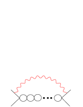
Figure 2: A radiation pion graph with $n$ internal $C_{0}$ bubbles.

which contains $n$ nucleon bubbles inside a radiation pion loop. The loop integral in this graph vanishes if the pion pole is not taken so there is no potential pion contribution. Emission of the radiation pion in these graphs changes the spin/isospin of the nucleon pair. Therefore, if the external nucleons are in a spin-triplet (singlet) state, then the coefficients appearing in the internal bubble sum are $C_{0}^{S}\>(C_{0}^{T})$. For definiteness, consider nucleon-nucleon scattering in the ${}^{1}S_{0}$ channel. The contribution from the graph in Fig. 2 is:

$${g_{A}^{2}\over 2f^{2}}\int\!\!{d^{4}q\over(2\pi)^{4}}{i\over q_{0}+i\epsilon}\>{i\over q_{0}+i\epsilon}\>{-i\,{\vec{q}\,}^{2}\over q_{0}^{2}-{\vec{q}\,}^{2}-m_{\pi}^{2}+i\epsilon}[-iC_{0}^{T}(\mu_{R})]^{n+1}$$

$$\qquad\qquad\times\left[\int\!\!{d^{4}k\over(2\pi)^{4}}{i\over q_{0}-k_{0}+\frac{E}{2}-{({\vec{k}}-{\vec{q}\,})^{2}\over 2M}+i\epsilon}\>{i\over k_{0}+\frac{E}{2}-{{\vec{k}}^{2}\over 2M}+i\epsilon}\right]^{n}\,.$$

The $q_{0}$ integral is closed around the one pion pole above the real axis so $q_{0}\sim|{\vec{q}\,}|\sim Q$. In the $k_{0}$ integrals a nucleon pole must be taken. In the KSW power counting, $k_{0}\sim Q^{2}/M,|{\vec{k}\,}|\sim Q$. The graph then scales as $(Q/M)^{n+1}$. This suggests that graphs with nucleon bubbles inside the radiation loop are suppressed relative to the one loop radiation pion graph. However, explicitly performing the $q_{0}$ and $k_{0}$ integrals gives

$$-iC_{0}^{T}(\mu_{R})\,{g_{A}^{2}\over 2f^{2}}\!\!\int\!\!\!{d^{3}q\over(2\pi)^{3}}{{\vec{q}\,}^{2}\over({\vec{q}\,}^{2}+m_{\pi}^{2})^{3/2}}\left[\int\!\!{d^{3}k\over(2\pi)^{3}}{-MC_{0}^{T}(\mu_{R})\over{\vec{k}\,}^{2}+M({\vec{q}\,}^{2}+m_{\pi}^{2})^{1/2}-ME}\right]^{n}\!\!\!\!.$$

The size of the loop momenta $k$ in the nucleon bubbles is $\sim\sqrt{Mm_{\pi}}$ even for $p<\sqrt{Mm_{\pi}}$. The integral will be dominated by ${\vec{q}\,}\sim m_{\pi}$ so the graph will scale as

$${1\over\Lambda_{\chi}^{2}}\>{m_{\pi}^{2}\over M\mu_{R}}\bigg{(}{\sqrt{Mm_{\pi}}\over\mu_{R}}\bigg{)}^{n}\,.$$

(Recall $\Lambda_{\chi}=4\pi f$). For $\mu_{R}\sim Q\sim m_{\pi}$, we see that graphs with additional bubbles are enhanced, contrary to the KSW power counting. The sum over graphs with an arbitrary number of bubbles is $\mu_{R}$ independent and the correct estimate for the size is obtained when $\mu_{R}\sim\sqrt{Mm_{\pi}}$. At this scale, these graphs and their sum are of order $m_{\pi}^{3/2}/(M^{3/2}\Lambda_{\chi}^{2})=Q_{r}^{3}/(M^{3}\Lambda_{\chi}^{2})$.

In the KSW power counting, one assumes the loop momentum in the nucleon bubbles is dominated by $k\sim Q,k_{0}\sim Q^{2}/M$. However, when the nucleon bubbles are inside a radiation pion loop, the energy flowing into the nucleon bubbles is actually order $m_{\pi}$, and therefore $k^{0}\sim m_{\pi}$ and $k\sim\sqrt{Mm_{\pi}}\equiv Q_{r}$. This scale corresponds to the threshold for on-shell pion production.

In general, radiation pion graphs will depend on $p$, $m_{\pi}$ and $M$ in a complicated way, making them difficult to power count if one takes $p\sim m_{\pi}$. However, the natural scale for loop momenta with radiation pions is $Q_{r}$, and the power counting simplifies considerably if we consider nucleons scattering at $p\sim Q_{r}$. Later we will discuss what happens as $p$ is lowered back down to $m_{\pi}$.

Power counting at the scale $Q_{r}$ is straightforward. We take $p\sim\mu_{R}\sim Q_{r}$. The $C_{2n}$ scale with $\mu_{R}$ exactly the same way as in the KSW power counting, $C_{2n}p^{2n}\sim p^{2n}/\mu_{R}^{n+1}\sim Q_{r}^{n-1}$. A radiation pion propagator gives $M^{2}/Q_{r}^{4}$, the pion nucleon coupling gives $Q_{r}^{2}/M$. Nucleon propagators scale like $M/Q_{r}^{2}$. In a radiation loop $q_{0}\sim|{\vec{q}}\,|\sim m_{\pi}$, so the loop measure $d^{4}q\sim Q_{r}^{8}/M^{4}$. The measure of a potential loop scales as $Q_{r}^{5}/M$. Using this power counting it is straightforward to show that all graphs with one radiation pion and an arbitrary number of $C_{0}$’s scale as $Q_{r}^{3}/(M^{3}\Lambda_{\chi}^{2})$. These graphs are shown in Fig. 3.

Figure 3: Leading order radiation pion graphs for $NN$ scattering. The solid lines are nucleons, the wavy lines are radiation pions and $\delta M$, $\delta Z$ are the mass and field renormalization counterterms. The filled dot denotes the $C_{0}(\mu_{R})$ bubble chain. There is a further field renormalization contribution that is not shown, but is included in the calculation.$\!{}^{{\bf?}}$

It is interesting to examine the result of evaluating some of the diagrams in Fig. 3 explicitly $\!{}^{{\bf?}}$ $(\bar{\mu}^{2}=\mu^{2}\pi e^{-\gamma_{E}})$:

$$a) = -3i{\cal A}_{-1}{g_{A}^{2}m_{\pi}^{2}\over(4\pi f)^{2}}\bigg{[}{1\over\epsilon}+{1\over 3}-{\rm ln}\Big{(}{m_{\pi}^{2}\over{\overline{\mu}}^{2}}\Big{)}\bigg{]}\,,$$ (2)

$$b) = [{\cal A}_{-1}]\,^{2}\,{g_{A}^{2}Mm_{\pi}^{2}\over(4\pi f)^{2}}\,\Bigg{\{}{3\,p\over 4\pi}\,\bigg{[}{1\over\epsilon}+{7\over 3}-2\,{\rm ln}\,2-{\rm ln}\Big{(}{m_{\pi}^{2}\over{\overline{\mu}}^{2}}\Big{)}-{\rm ln}\Big{(}{-p^{2}\over{\overline{\mu}}^{2}}\Big{)}\bigg{]}$$

$$\qquad\qquad\qquad\qquad+{i\sqrt{Mm_{\pi}}\over 4\sqrt{\pi}}\,I_{1}\Big{(}{E\over m_{\pi}}\Big{)}\Bigg{\}}\,,$$

$$c) = {ig_{A}^{2}\over\sqrt{\pi}f^{2}}\Big{(}{m_{\pi}\over M}\Big{)}^{3/2}I_{2}\Big{(}{E\over m_{\pi}}\Big{)}\,.$$

$I_{1}$ and $I_{2}$ are hypergeometric functions. The $1/\epsilon$ poles are cancelled by insertions of a $D_{2}m_{\pi}^{2}$ counterterm. The leading order amplitude

$${\cal A}_{-1}=-{4\pi\over M}{1\over 1/a^{S}+ip}\,,$$

scales as $\sim 1/(Mp)$, so we see that Eq. (2) has terms proportional to

$$\left({m_{\pi}\over M}\right)^{3/2}\!\!\!\!\!\!,\qquad{m_{\pi}^{2}\over Mp}\qquad{\rm and}\qquad{m_{\pi}^{5/2}\over M^{1/2}p^{2}}\,.$$

For $p\sim Q_{r}$ these terms scale as $Q_{r}^{3}/M^{3}$, as anticipated by the power counting. At $p\sim m_{\pi}\sim Q$, these terms scale like $(Q/M)^{3/2},Q/M$, and $(Q/M)^{1/2}$ respectively. Bubble sums which do not appear inside radiation loops will be referred to as external bubble sums. These bubble sums are responsible for the factors of $p$ in the denominators, and thus the enhancement of some terms at low momentum. Graphs with two external bubble sums have terms that are enhanced by $Q_{r}^{2}/Q^{2}\sim 1/m_{\pi}$ (and $Q_{r}/Q\sim 1/\sqrt{m_{\pi}}$), while graphs with one external bubble sum have terms enhanced by $1/\sqrt{m_{\pi}}$. Individual graphs like $b)$ have parts that scale differently with $Q$. Terms which scale like $Q^{1/2}$ at low $p$ are actually larger than NNLO in the $Q$ counting. The $Q^{1/2}$ contributions come from graphs $b),e)$ and $f)$, and cancel when the graphs are added together. Presently it is not known whether this cancellation occurs for some reason or is merely an accident.

The sum of all $Q_{r}^{3}$ graphs is:

$$i\,{\cal A}^{rad} = 6i\,{\cal A}_{-1}^{2}{g_{A}^{2}m_{\pi}^{2}\over(4\pi f)^{2}}\,{M\over 4\pi}\left({1\over a^{S}}-{1\over a^{T}}\right)\,\bigg{[}\kappa+{\rm ln}\Big{(}{{\mu}^{2}\over m_{\pi}^{2}}\Big{)}\bigg{]}$$ (3)

$$+i\,{\cal A}_{-1}^{2}\left({M\over 4\pi}\right)^{2}\left({1\over a^{S}}-{1\over a^{T}}\right)^{2}{g_{A}^{2}\over\sqrt{\pi}f^{2}}\Big{(}{m_{\pi}\over M}\Big{)}^{3/2}I_{2}\Big{(}{E\over m_{\pi}}\Big{)}\,,$$

where the $\ln(\mu)$ dependence is cancelled by $D_{2}(\mu)$. (For the ${}^{3}S_{1}$ channel, the result is the same as above with $a_{S}\leftrightarrow a_{T}$.) The final answer turns out to be much smaller than anticipated by the power counting. For $p\sim Q_{r}$, the first term is suppressed by a factor of $1/Q_{r}(1/a^{S}-1/a^{T})$, the second by $1/Q_{r}^{2}(1/a^{S}-1/a^{T})^{2}$. This suppression occurs because the radiation pions couple to a charge of Wigner’s $SU(4)$, which is a symmetry of the leading order Lagrangian in the limit $a_{S},a_{T}\rightarrow\infty$ (or $a_{S}=a_{T}$).$\!{}^{{\bf?},{\bf?}}$ The order $Q_{r}^{3}$ radiation pion graphs are a tiny correction to the S-wave scattering amplitude.

The next important radiation pion contribution comes from graphs with one insertion of a $C_{2}p^{2}$, $D_{2}m_{\pi}^{2}$, or $G_{2}$ operator $\!{}^{{\bf?}}$ or a potential pion, and one radiation pion with an arbitrary number of $C_{0}$’s. Power counting these graphs gives $Q_{r}^{4}/(M^{3}\Lambda_{\chi}^{2}\Lambda)$, i.e. these are suppressed by $Q_{r}/\Lambda$ relative to the leading radiation pion graphs in Fig. 3. Note that $Q_{r}=360\,{\rm MeV}$, so for the most pessimistic estimates of $\Lambda$, the $Q_{r}/\Lambda$ expansion does not converge. If this is the case then the radiation pion contribution is incalculable. This is true of radiation contributions even when we scale down to $p\sim m_{\pi}$. However, at the low momenta where the theory would be applicable, the radiation pions could be integrated out. For example, the hypergeometric function $I_{2}(E/m_{\pi})=I_{2}(p^{2}/(Mm_{\pi}))$ could be expanded in a series in $p^{2}$ and the effect of each term absorbed into the definition of a $C_{2n}$. Assuming the radiation pion contribution is computable, the $Q_{r}^{4}$ correction is almost certainly larger than the $Q_{r}^{3}$ correction. Since the $C_{2}p^{2}$, $D_{2}m_{\pi}^{2}$ operators and potential pion exchange do not respect Wigner’s $SU(4)$, there will be no suppression by factors of $1/(a\,Q_{r})$.

An important issue which needs to be addressed is how the radiation pions graphs scale as $p$ is lowered from $Q_{r}$ to $m_{\pi}$. We saw that the $Q_{r}^{3}$ graphs had pieces that scaled as $Q^{1/2},Q$, $Q^{3/2},\ldots$, for $p\sim m_{\pi}$, and that this enhancement can be understood by counting the number of external bubble sums. In order to know which radiation pion graphs to include at a given order in the KSW power counting, we must know how a $Q_{r}^{n}$ correction scales with $Q$ for $p\sim m_{\pi}$. It turns out that an order $Q_{r}^{n}$ calculation is sufficient to determine the order $Q^{n/2-1}$ result.

To see this first consider the $Q$ expansion of $p\,{\rm cot}\,\delta$:

$$p\,{\rm cot}\,\delta = ip+{4\pi\over M}{1\over{\cal A}}$$

$$= ip+{4\pi\over M}{1\over{\cal A}_{-1}}-{4\pi\over M}{{\cal A}_{0}\over{\cal A}_{-1}^{2}}-{4\pi\over M}\left({{\cal A}_{1}\over{\cal A}_{-1}^{2}}-{{\cal A}_{0}^{2}\over{\cal A}_{-1}^{3}}\right)$$

$$-{4\pi\over M}\left({{\cal A}_{2}\over{\cal A}_{-1}^{2}}-{2{\cal A}_{0}{\cal A}_{1}\over{\cal A}_{-1}^{3}}+{{\cal A}_{0}^{3}\over{\cal A}_{-1}^{4}}\right)+\dots\,.$$

$p\,{\rm cot}\,\delta$ is real and an analytic function of $p^{2}$ near $p=0$. This will be true order by order in $Q$ so:

$${{\cal A}_{0}\over{\cal A}_{-1}^{2}}=f_{0}\, \Rightarrow \,{\cal A}_{0}=f_{0}{\cal A}_{-1}^{2}\,,$$

$${{\cal A}_{1}\over{\cal A}_{-1}^{2}}-{{\cal A}_{0}^{2}\over{\cal A}_{-1}^{3}}=f_{1}\, \Rightarrow \,{\cal A}_{1}=f_{1}{\cal A}_{-1}^{2}+f_{0}^{2}{\cal A}_{-1}^{3}\,,$$

$${{\cal A}_{2}\over{\cal A}_{-1}^{2}}-{2{\cal A}_{0}{\cal A}_{1}\over{\cal A}_{-1}^{3}}+{{\cal A}_{0}^{3}\over{\cal A}_{-1}^{4}}=f_{2}\, \Rightarrow \,{\cal A}_{2}=f_{2}{\cal A}_{-1}^{2}+2f_{0}f_{1}{\cal A}_{-1}^{3}+f_{0}^{3}{\cal A}_{-1}^{4}\,,$$

where the $f_{n}$ are real functions of $p$ which are analytic about $p^{2}=0$. We see that the general form of a higher order amplitude is powers of ${\cal A}_{-1}$ multiplied by functions of $p$. The crucial point is that the function multiplying the ${\cal A}_{-1}^{2}$ is the only new contribution. The coefficient of ${\cal A}_{-1}^{n},n>2$, is determined by lower order amplitudes. In the $Q$ expansion of $p\,{\rm cot}\,\delta$ the latter contributions will cancel.

This generalizes to the $Q_{r}$ expansion of radiation pion graphs, the only difference being that the radiation pion contribution starts out at $Q_{r}^{3}$, while the potential pion starts out at $Q_{r}^{0}$. A $Q_{r}^{n}$ radiation pion correction to the amplitude will be of the form:

$${\cal A}_{n}={\cal A}_{-1}^{2}f_{n,2}+{\cal A}_{-1}^{3}f_{n,3}+\ldots+{\cal A}_{-1}^{n-1}f_{n,n-1}.$$

Again, the $f_{n,m}$ are analytic about $p^{2}=0$ and all the $f_{n,m}$ except for $f_{n,2}$ will be determined from lower order amplitudes. Since ${\cal A}_{n}\sim Q_{r}^{n}$ and ${\cal A}_{-1}\sim 1/(Mp)$, $f_{n,m}\sim Q_{r}^{n+m}$ for $p\sim Q_{r}$. To understand how $f_{n,m}$ scales with $Q$ as $p$ is lowered to $m_{\pi}$, note that without loss of generality, $f_{n,m}$ can be written as

$$f_{n,m}={({\sqrt{Mm_{\pi}}})^{n+m}\over\Lambda_{\chi}^{2}\ {\overline{\Lambda}}^{\>n-m}}{\hat{f}}_{n,m}\left({p\over\sqrt{Mm_{\pi}}},\ldots\right)\,,$$

where the ellipses denote momentum dependence that involves scales other than $Q_{r}$, and ${\overline{\Lambda}}=\Lambda_{\chi}$, $\Lambda$, or $M$. For $p\sim m_{\pi}$ the ellipse denote dependence on the dimensionless variables $p/m_{\pi}$, $pa$, and $p/{\overline{\Lambda}}$. For $p\sim m_{\pi}$, ${p/\sqrt{Mm_{\pi}}}\sim(Q/M)^{1/2}$ and the function ${\hat{f}}_{n,m}$ can be expanded in its first argument:

$${\cal A}_{-1}^{m}f_{n,m}={\cal A}_{-1}^{m}{({\sqrt{Mm_{\pi}}})^{n+m}\over\Lambda_{\chi}^{2}\ {\overline{\Lambda}}^{\>n-m}}{\hat{f}}_{n,m}\left(0,\ldots\right)\left[1+O\left({Q\over M}\right)^{1/2}\right]\,.$$

The leading term scales as $\sim Q^{n/2-m/2}$ for $p\sim m_{\pi}\sim Q$. Since only the $m=2$ term actually ends up contributing to $p\,{\rm cot}\,\delta$, the new contribution at $Q_{r}^{n}$ scales like $Q^{n/2-1}$ (plus subleading terms) for $p\sim m_{\pi}$. This is consistent with the result of the $Q_{r}^{3}$ calculation, where the largest contributions from individual graphs scaled as $Q^{1/2}$. A cancellation between graphs resulted in this contribution vanishing. The remaining terms scale as $Q$, $Q^{3/2},\ldots$ (counting $1/a\sim Q$). The $Q_{r}^{n}$ radiation pion contribution could have a $Q^{1/2}$ contribution from the ${\cal A}_{-1}^{n-1}f_{n,n-1}$ term. But this contribution is determined by the $Q_{r}^{3}$ amplitude which vanished; so there will be no $Q^{1/2}$ contribution from any radiation pion graph. For example, at $Q_{r}^{4}$ the terms proportional to ${\cal A}_{-1}^{3}$ comes from graphs such as those shown in Fig. 4.

Figure 4: Example of order $Q_{r}^{4}$ graphs that have three external bubble sums.

These graphs factorize into two pieces which are lower order and it is easy to see that the same cancellation between the $Q^{1/2}$ pieces of the graphs $b),e)$ and $f)$ will also occur at $Q_{r}^{4}$.

Since $Q^{n/2-1}=Q$ for $n=4$, the $Q_{r}^{4}$ radiation pion graphs may have a contribution that is NNLO for $p\sim m_{\pi}$. We have checked that graphs with one insertion of the $D_{2}m_{\pi}^{2}$ operator do not give rise to such a contribution, but a calculation of the remaining $Q_{r}^{4}$ graphs has not been performed. These graphs need to be computed in order to obtain the complete NNLO amplitude. Unfortunately, graphs with one potential and one radiation pion are numerous. Higher $Q_{r}^{n}$ amplitudes may have a contribution which scales as $Q$ for $p\sim m_{\pi}$ from the ${\cal A}_{-1}^{n-2}f_{n,n-2}$ term. But these will cancel in the $Q$ expansion of $p\,{\rm cot}\,\delta$. Note that a calculation of the order $Q_{r}^{5}$ graphs would be necessary to determine the order $Q^{3/2}$ terms.

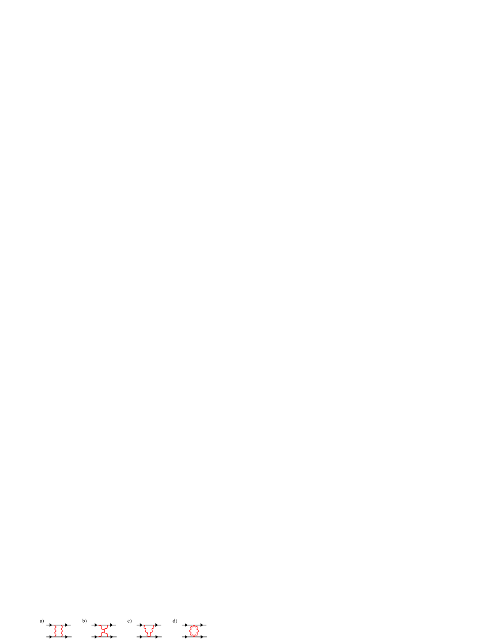
Figure 5: Examples of one-loop graphs which have soft pion contributions. Graphs a)-d) also have a radiation pion contribution, while in addition graph a) has a potential pion contribution.

Finally, we briefly discuss soft contributions. These first arise in box-type diagrams with two pions, such as those shown in Fig. 5. Dressing these graphs on the outside with $C_{0}$ bubbles gives further diagrams of the same order. Unlike radiation graphs, which are dominated by loop momenta $|\vec{q}\,|\sim m_{\pi}$, the box-like diagrams receive nonvanishing contributions from $|\vec{q}\,|\sim Q_{r}$. It is this latter type of contribution which is called soft. In soft loops the measure $d^{4}q\sim Q_{r}^{4}$ instead of $Q_{r}^{8}/M^{4}$. For nucleon propagators in soft loops, the loop energy is always greater than the nucleon’s kinetic energy, so the propagator is static (like heavy quark effective theory propagators, see $\!{}^{{\bf?}}$ or $\!{}^{{\bf?}}$). These propagators scale as $1/Q_{r}$. Pion propagators scale as $1/Q_{r}^{2}$ and pion-nucleon vertices give a factor of $Q_{r}$. Power counting the graphs in Fig. 5 gives $\sim Q_{r}^{2}$ for the soft contribution and $\sim Q_{r}^{4}/M^{2}$ for the radiation contribution. The contribution from each regime can be separated using the method of asymptotic expansions $\!{}^{{\bf?},{\bf?},{\bf?}}$ and explicit evaluation $\!{}^{{\bf?}}$ of the graphs verifies the power counting appropriate for each type of contribution. At $p\sim Q_{r}$, the soft contribution actually dominates all radiation pion graphs we have considered so far. However, for $p\sim m_{\pi}$ these soft graphs are order $Q^{2}$, and therefore are not enhanced by the scaling down to $p\sim m_{\pi}$. The leading order soft graphs are ${\rm N}^{3}{\rm LO}$ in the KSW power counting.

NNLO Calculation of the ${}^{1}S_{0}$ Phase Shift

In this section, we present a partial NNLO calculation of the ${}^{1}S_{0}$ phase shift. A more detailed analysis will be given in a future publication.$\!{}^{{\bf?}}$ The first piece of the $Q_{r}^{3}$ radiation pion contribution in Eq. (3) is order $Q$. The second term is order $Q^{3/2}$ and is not included in the NNLO calculation. The relativistic corrections are computed in Ref.$\!{}^{{\bf?}}$ and shown to be negligible. This is because they are suppressed relative to the leading order amplitude by $(Q/M)^{2}$ rather than $(Q/\Lambda)^{2}$ and so are smaller than other NNLO corrections. The calculation here includes order $Q$ contact interactions and potential pion graphs. The NNLO calculation is incomplete because of the omission of the $Q_{r}^{4}$ radiation pion graphs, as discussed in the previous section. The pieces of the NNLO amplitude which are included are expected to scale as $Q/(M\Lambda^{2})$ while the $Q_{r}^{4}$ radiation pion graphs are expected to scale as $Q/(\Lambda_{\chi}^{2}\Lambda)$ for $p\sim m_{\pi}$. Since $\Lambda<\Lambda_{\chi}\approx M$, the contribution from $Q_{r}^{4}$ radiation pion graphs may be smaller than what has been included.

Since we are only interested in the ${}^{1}S_{0}$ channel, only $s=S$ operators are relevant and this superscript will be omitted in the following discussion. At NNLO, the following terms are added to the Lagrangian in Eq. (Radiation and Soft Pions):

$${\cal L}= -{C_{4}\over 64}\left[(N^{T}P_{i}N)^{\dagger}(N^{T}P_{i}\>{\stackrel{{\scriptstyle\leftrightarrow}}{{\nabla}}}^{\,4}N)+h.c.+2(N^{T}P_{i}{\stackrel{{\scriptstyle\leftrightarrow}}{{\nabla}}}^{\,2}N)^{\dagger}(N^{T}P_{i}\>{\stackrel{{\scriptstyle\leftrightarrow}}{{\nabla}}}^{\,2}N)\right]$$ (4)

$$+{E_{4}\over 8}\omega{\rm Tr}(m^{\xi})\left[(N^{T}P_{i}N)^{\dagger}(N^{T}P_{i}\>{\stackrel{{\scriptstyle\leftrightarrow}}{{\nabla}}}^{\,2}N)+h.c.\right]$$

$$-{D_{4}\over 2}\omega^{2}\Big{\{}{\rm Tr}^{2}(m^{\xi})+2{\rm Tr}[(m^{\xi})^{2}]\Big{\}}(N^{T}P_{i}N)^{\dagger}(N^{T}P_{i}N)\,,$$

where only terms relevant for the phase shift are included and isospin violation is neglected. All calculations presented in this section will be done in the PDS renormalization scheme $\!{}^{{\bf?},{\bf?}}$ with spin and isospin traces done in four dimensions.

There are six coefficients that appear at NNLO: $C_{0}$, which is present in the leading order calculation, $C_{2}$ and $D_{2}$, which first appear at NLO, and $C_{4},E_{4}$, and $D_{4}$. It is important that the coupling constants are expanded in $Q$: $\!{}^{{\bf?}}$

$$C_{0} \rightarrow C_{0}+C_{0,0}+C_{0,1}$$

$$C_{2} \rightarrow C_{2}+C_{2,-1}$$

$$D_{2} \rightarrow D_{2}+D_{2,-1}\,.$$ (5)

The first piece of $C_{0}$ is treated nonperturbatively (i.e. $C_{0}\sim Q^{-1}$), while $C_{0,0}\sim Q^{0},C_{0,1}\sim Q$. Solving the renormalization group equations (RGE) for the couplings perturbatively ensures that the amplitude is $\mu$ independent order by order in the expansion. Therefore, theoretical expressions for physical quantities, such as the scattering length or the location of the pole, are always $\mu$ independent. Physically, the $Q$ expansion of the couplings is a consequence of the fact that higher order loop graphs with pions can renormalize the short distance operators at different orders in $Q$, and therefore different values of the couplings will be obtained at different orders in the expansion.

When a coupling is expanded in $Q$ and its RGE solved perturbatively, a new constant of integration is obtained for each term in the expansion. For example, the RGE for $C_{0}$ is:

$$\mu{\partial\over\partial\mu}C_{0} = {M\mu\over 4\pi}\left(C_{0}+{g_{A}^{2}\over 2f^{2}}\right)^{2}\,.$$ (6)

After the perturbative expansion of $C_{0}$ this becomes

$$\mu{\partial\over\partial\mu}C_{0}={M\mu\over 4\pi}C_{0}^{2}\,,\qquad\mu{\partial\over\partial\mu}C_{0,0}=2{M\mu\over 4\pi}C_{0}\left(C_{0,0}+{g_{A}^{2}\over 2f^{2}}\right),$$

$$\mu{\partial\over\partial\mu}C_{0,1}={M\mu\over 4\pi}\left[2\,C_{0}\,C_{0,1}+\left(C_{0,0}+{g_{A}^{2}\over 2f^{2}}\right)^{2}\>\right],\,\,\,\,\,\,$$

with solutions

$$C_{0}={4\pi\over M}{1\over-\mu+\gamma}\,,\qquad C_{0,0}={M\kappa\over 4\pi}\,C_{0}^{2}-{g_{A}^{2}\over 2f^{2}}\,,$$

$$C_{0,1}={1\over C_{0}}\left(C_{0,0}+{g_{A}^{2}\over 2f^{2}}\right)^{2}+{M\kappa^{\prime}\over 4\pi}\>C_{0}^{2}\,.$$ (7)

Three constants of integration appear: $\gamma,\kappa$ and $\kappa^{\prime}$; one for each term in the $Q$ expansion of $C_{0}$. For consistency we must assign these constants a $Q$ counting. For instance, $C_{0,0}$ has a term in its solution $\kappa\,C_{0}^{2}\sim\kappa/\mu^{2}$. Since $C_{0,0}\sim Q^{0}$, $\kappa$ must be of order $Q^{2}$. This reflects the fact that $\kappa$ is intrinsically small. In the theory without pions, $\kappa=\gamma-1/a$. As we will see below, the values of $\gamma,\kappa,\kappa^{\prime}$ may be fixed by demanding that the amplitude has the correct pole structure. In this case, $\kappa\approx r_{0}/(2a^{2})\sim Q^{2}$. The results in Eq. (NNLO Calculation of the ${}^{1}S_{0}$ Phase Shift) can also be obtained by solving Eq. (6) exactly and expanding the result (including the constant of integration) in $Q$. Because of the perturbative expansion of the couplings in Eq. (NNLO Calculation of the ${}^{1}S_{0}$ Phase Shift) there are ten constants of integration at NNLO. However, the NNLO amplitude will depend only on six independent linear combinations of these constants. There are two further constraints on the number of free parameters: 1) at this order, $C_{4}$, $E_{4}$ and $D_{4}$ are determined entirely in terms of lower order couplings; 2) spurious double and triple poles in the NLO and NNLO amplitudes must be cancelled in order to obtain a good fit.

The fact that $C_{4}$, $E_{4}$ and $D_{4}$ are determined in terms of lower order couplings is a consequence of solving the RGE’s and applying the KSW power counting. For instance $\!{}^{{\bf?}}$, the RGE for $C_{4}$ is:

$$\mu{\partial\over\partial\mu}C_{4} = {M\mu\over 4\pi}\left(2\,C_{0}\,C_{4}+C_{2}^{2}\right),$$

which has the solution

$$C_{4}={C_{2}^{2}\over C_{0}}+\rho{M\over 4\pi}C_{0}^{2}\,,$$

where $\rho$ is a constant of integration. In the theory without pions, $\rho$ is proportional to the shape parameter, which is $\sim Q^{0}$ in the KSW power counting. It is also reasonable to consider $\rho\sim Q^{0}$ in the theory with pions, since $\rho$ is a constant of integration in the RGE for the lowest order term in the $Q$ expansion of $C_{4}$. Therefore, $C_{2}^{2}/C_{0}\sim Q^{-3}$, while $\rho C_{0}^{2}M/(4\pi)\sim Q^{-2}$. The second term is subleading in the $Q$ expansion, and should be omitted at NNLO, so $C_{4}=C_{2}^{2}/C_{0}$. Similar relations for $E_{4},D_{4}$ hold at NNLO:

$$E_{4}={2C_{2}D_{2}\over C_{0}}\,,\qquad\quad D_{4}={D_{2}^{2}\over C_{0}}\,.$$

It is interesting to note that these relations arise even though there are $\ln(\mu^{2})$ terms in the amplitude which contribute to the beta functions for $E_{4}$ and $D_{4}$.

Because of the nonperturbative treatment of $C_{0}$, spurious poles arise at higher orders in the expansion. The leading order amplitude ${\cal A}_{-1}$ has a simple pole at $p=i\gamma$. The NLO calculation is proportional to ${\cal A}_{-1}^{2}$, and therefore has a double pole, while the NNLO amplitude has terms proportional to ${\cal A}_{-1}^{2}$ and ${\cal A}_{-1}^{3}$. To obtain a good fit at low momentum, parameters need to be fixed so that the amplitude has only a simple pole at each order in the expansion. This requires that ${\cal A}_{-1}$ have its pole in the correct location and that the residues of the spurious double and triple poles vanish. This requirement leads to the following good fit conditions: $\!{}^{{\bf?}}$

$$\left.{1\over{\cal A}_{-1}}\right|_{p=p^{*}}\!\!\!\!\!\!\!\!\!=0\,,\qquad\left.{{\cal A}_{0}\over{\cal A}_{-1}^{2}}\right|_{p=p^{*}}\!\!\!\!\!\!\!\!\!=0\,,\qquad\left.{{\cal A}_{1}\over{\cal A}_{-1}^{2}}\right|_{p=p^{*}}\!\!\!\!\!\!\!\!\!=0\,,\qquad$$ (8)

where $p^{*}$ is the location of the physical pole. The second condition first appears at NLO, the third at NNLO. The residue of the triple pole in ${\cal A}_{1}$ is cancelled by the second equation in Eq. (8). The first equation results in $\gamma=-ip^{*}$, while the other equations give constraints which eliminate two of the remaining parameters. Eq. (8) will also apply in the ${}^{3}S_{1}$ channel.

Figure 6: Order $Q$ contact interaction and potential pion graphs for the ${}^{1}S_{0}$ channel. The shaded circle denotes a $C_{0}$ bubble sum. At this order the first six graphs cancel each other as explained in the text.

The graphs evaluated in the NNLO calculation are shown in Fig. 6. The final result is surprisingly simple. The amplitude up to NNLO is:

$${\cal A}_{-1} = -{4\pi\over M}{1\over\gamma+ip}\,,$$

$${{\cal A}_{0}} = -{\cal A}_{-1}^{2}(\zeta_{1}\,p^{2}+\zeta_{2}\,m_{\pi}^{2})$$

$$+{g_{A}^{2}\over 2f^{2}}{\cal A}_{-1}^{2}\Big{(}{Mm_{\pi}\over 4\pi}\Big{)}^{2}\bigg{[}{(\gamma^{2}-p^{2})\over 4p^{2}}{\rm ln}\Big{(}1+{4p^{2}\over m_{\pi}^{2}}\Big{)}-\,{\gamma\over p}{\rm tan}^{-1}\left({2p\over m_{\pi}}\right)\bigg{]}\,,$$

$${{\cal A}_{1}} = {{\cal A}_{0}^{2}\over{\cal A}_{-1}}-{\cal A}_{-1}^{2}\Big{(}\zeta_{3}\,m_{\pi}^{2}+\zeta_{4}\,p^{2}+\zeta_{5}{p^{4}\over m_{\pi}^{2}}\Big{)}+{{\cal A}_{0}}{Mg_{A}^{2}\over 8\pi f^{2}}\,{m_{\pi}^{2}\over p}\bigg{[}{\gamma\over 2p}\>{\rm ln}\Big{(}1+{4p^{2}\over m_{\pi}^{2}}\Big{)}$$

$$-{\rm tan}^{-1}\Big{(}{2p\over m_{\pi}}\Big{)}\bigg{]}+{M{\cal A}_{-1}^{2}\over 4\pi}\Big{(}{Mg_{A}^{2}\over 8\pi f^{2}}\Big{)}^{2}{m_{\pi}^{4}\over 4p^{3}}\Bigg{\{}2(\gamma^{2}-p^{2})\,{\rm Im}\,{\rm Li_{2}}\Big{(}{-m_{\pi}\over m_{\pi}-2ip}\Big{)}$$

$$-4\gamma\,p\>{\rm Re}\,{\rm Li_{2}}\Big{(}{-m_{\pi}\over m_{\pi}-2ip}\Big{)}-{\gamma\,p\,\pi^{2}\over 3}-(\gamma^{2}+p^{2})\bigg{[}{\rm Im}\,{\rm Li_{2}}\Big{(}{m_{\pi}+2ip\over-m_{\pi}+2ip}\Big{)}$$

$$+{\gamma\over 4p}\ln^{2}\Big{(}1+\frac{4p^{2}}{m_{\pi}^{2}}\Big{)}-\tan^{-1}\Big{(}\frac{2p}{m_{\pi}}\Big{)}\ln\Big{(}1+\frac{4p^{2}}{m_{\pi}^{2}}\Big{)}\bigg{]}\Bigg{\}}\,.$$

Using this amplitude it is easy to verify that the S-matrix is unitary to the order we are working. The six linearly independent constants appearing in the amplitude are $\gamma,\zeta_{1},\zeta_{2},\zeta_{3},\zeta_{4},\zeta_{5}$. By definition $\zeta_{1}-\zeta_{5}$ are dimensionless. They are given in terms of coupling constants in the Appendix.

For the ${}^{1}S_{0}$ channel, the location of the pole is determined by solving

$$-{1\over a}+{r_{0}\over 2}(p^{*})^{2}-ip^{*}=0\,.$$ (10)

Adding the shape parameter correction to Eq. (10) changes the location of the pole by less than $0.01\%$, so this approximation for the physical pole location is sufficiently accurate. Eq. (10) has a solution for $p^{*}=-i\,7.877\,{\rm MeV}$, which fixes the single LO parameter, $\gamma=-7.877\,{\rm MeV}$. The NLO good fit condition relates the constants $\zeta_{1}$ and $\zeta_{2}$,

$$-\zeta_{1}\gamma^{2} + \zeta_{2}m_{\pi}^{2}+{Mm_{\pi}^{2}\over 4\pi}{g_{A}^{2}M\over 8\pi f^{2}}\left[{1\over 2}{\rm log}\left(1-{4\gamma^{2}\over m_{\pi}^{2}}\right)-{\rm tanh}^{-1}\left({2\gamma\over m_{\pi}}\right)\right]=0$$ (11)

$$\Rightarrow \zeta_{2}={\gamma^{2}\over m_{\pi}^{2}}\,\zeta_{1}+{M\over 4\pi}{g_{A}^{2}M\over 8\pi f^{2}}\left[-{2\gamma\over m_{\pi}}-{2\gamma^{2}\over m_{\pi}^{2}}+{\cal O}\Big{(}{\gamma^{3}\over m_{\pi}^{3}}\Big{)}\right]\,.$$

We can use this equation to eliminate $\zeta_{2}$ in favor of $\zeta_{1}$, leaving one new parameter in the fit at NLO. This good fit condition gives non-trivial $m_{\pi}$ dependence to the perturbative contributions to $C_{0}$ (such as $\kappa$) as emphasized in Refs. $\!{}^{{\bf?},{\bf?},{\bf?}}$. $\zeta_{1}$ is fixed by doing a weighted least squares fit to low momentum data. Note that $\zeta_{1}$ appears in the good fit condition multiplied by $\gamma^{2}$. Therefore, the value of $\zeta_{2}$ is insensitive to the value of $\zeta_{1}$ obtained from the fitting procedure. To a good degree of accuracy we can ignore $\zeta_{1}$ in Eq. (11), and then we find $\zeta_{2}\approx 0.03$. $\zeta_{2}$ is small because it is proportional to $\gamma/m_{\pi}$.

At NNLO, $\zeta_{5}=0$ once we impose $C_{4}=C_{2}^{2}/C_{0}$. The condition in Eq. (11) must still be satisfied. The NNLO good fit condition involves $\zeta_{3}$ and $\zeta_{4}$,

$$\zeta_{3} = \frac{\gamma^{2}}{m_{\pi}^{2}}\,\zeta_{4}+\Big{(}{Mg_{A}^{2}\over 8\pi f^{2}}\Big{)}^{2}{M\over 4\pi}\ {m_{\pi}^{2}\over\gamma}\bigg{[}{\rm Re}\,{\rm Li}\Big{(}{-m_{\pi}\over m_{\pi}+2\gamma}\Big{)}+\frac{\pi^{2}}{12}\bigg{]}$$

$$= \frac{\gamma^{2}}{m_{\pi}^{2}}\,\zeta_{4}+\Big{(}{Mg_{A}^{2}\over 8\pi f^{2}}\Big{)}^{2}{Mm_{\pi}\over 4\pi}\bigg{[}2\ln 2-(1+2\ln 2)\frac{\gamma}{m_{\pi}}+{\cal O}\Big{(}{\gamma^{2}\over m_{\pi}^{2}}\Big{)}\bigg{]}\,.$$

Since $\zeta_{4}$ is multiplied by $\gamma^{2}/m_{\pi}^{2}$, this condition basically fixes the value of $\zeta_{3}$. At this order $\zeta_{1}$ may change from its value at NLO. We have chosen to fix $\zeta_{1}$ and $\zeta_{4}$ by performing a least square fit to the lower momentum data.

Figure 7: Fit to the ${}^{1}S_{0}$ phase shift $\delta$ emphasizing the low momentum region. The solid line is the Nijmegen fit $\!{}^{{\bf?}}$ to the data (for $p>400\,{\rm MeV}$ values from the VPI $\!{}^{{\bf?}}$ phase shift analysis were used.). The long dashed, short dashed, and dotted lines are the LO, NLO, and NNLO results respectively. $\Delta\delta$ is the difference between these results and the solid line.

The ${}^{1}S_{0}$ phase shift is shown in Fig. 7. The solid line is the result of the Nijmegen phase shift analysis $\!{}^{{\bf?}}$. The ${}^{1}S_{0}$ phase shift has an expansion in powers of $Q$, and we have plotted the LO, NLO and NNLO results. The LO phase shift at $p\sim m_{\pi}$ is off by $49\%$. At NLO, the error is $14\%$. At NNLO, the error in the ${}^{1}S_{0}$ channel is less than $2\%$ at $p\sim m_{\pi}$, and the NNLO result gives improved agreement with the data even at $p\sim 400\,{\rm MeV}$.

Using $M=939\,{\rm MeV}$ and $m_{\pi}=137\,{\rm MeV}$, the parameters for our fit in the ${}^{1}S_{0}$ channel are:

$${\rm NLO}: \qquad\zeta_{1}=0.2163;\qquad\zeta_{2}=0.0318;$$

$${\rm NNLO}: \qquad\zeta_{1}=0.0777;\qquad\zeta_{2}=0.0313;\qquad\zeta_{3}=0.1831;\qquad\zeta_{4}=0.2447;$$

Note that $\zeta_{3}\sim Q$ is larger than $\zeta_{2}\sim Q^{0}$ because from Eqs. (11) and (NNLO Calculation of the ${}^{1}S_{0}$ Phase Shift), $\zeta_{3}/\zeta_{2}\sim m_{\pi}^{2}/(\gamma\Lambda_{NN})$. The parameter $\zeta_{2}$ is stable because it is fixed by the NLO good fit condition. On the other hand, $\zeta_{1}$ changes by a factor of 2.7 going from NLO to NNLO. One expects the value of coupling constants to change at each order in the expansion, but a factor of three difference is somewhat surprising. It is also disturbing that $\zeta_{4}$ is greater than $\zeta_{1}$, since, on the basis of the RGE, it is expected that $\zeta_{4}<\zeta_{1}$. At NNLO the RGE for $C_{2}$ is: $\!{}^{{\bf?}}$

$$\mu{\partial\over\partial\mu}C_{2} = 2{M\mu\over 4\pi}\left(C_{0}+{g_{A}^{2}\over 2f^{2}}\right)C_{2}\,.$$

Expanding $C_{2}$ perturbatively results in two equations:

$$\mu{\partial\over\partial\mu}C_{2} = 2{M\mu\over 4\pi}\,C_{0}\,C_{2}\,,$$ (13)

$$\mu{\partial\over\partial\mu}C_{2,-1} = 2{M\mu\over 4\pi}\left[\left(C_{0,0}+{g_{A}^{2}\over 2f^{2}}\right)C_{2}+C_{0}\,C_{2,-1}\right]\,,$$

with solutions

$$C_{2}=\zeta_{1}\,C_{0}^{2}\,,\qquad\quad C_{2,-1}=2{C_{2}\over C_{0}}\left(C_{0,0}+{g_{A}^{2}\over 2f^{2}}\right)+\zeta_{4}\,C_{0}^{2}\,.$$ (14)

The second term in $C_{2,-1}$ has exactly the same form as the leading $C_{2}$. $C_{2,-1}$ is supposed to be a perturbative correction to $C_{2}$, so $\zeta_{4}\sim Q<\zeta_{1}\sim Q^{0}$, and one does not expect this part of $C_{2,-1}$ to be significantly larger than the leading $C_{2}$.

Some insight into this puzzle can be obtained by comparing the NLO and NNLO expressions for $r_{0}$. Using Eq. (NNLO Calculation of the ${}^{1}S_{0}$ Phase Shift) we have

$$r_{0}^{NLO} = {8\pi\over M}\zeta_{1}+{2\over\Lambda_{NN}}\left(1-{8\gamma\over 3m_{\pi}}+{2\gamma^{2}\over m_{\pi}^{2}}\right)$$ (15)

$$= {8\pi\over M}(\zeta_{1}+0.2952)\,,$$

$$r_{0}^{NNLO} = {8\pi\over M}\left[\zeta_{4}+\zeta_{1}\left(1-{2m_{\pi}-2\gamma\over\Lambda_{NN}}\right)+{\zeta_{2}\over\Lambda_{NN}}\left({8m_{\pi}\over 3}-4\gamma\right)+\ldots\right]$$ (16)

$$= {8\pi\over M}(\zeta_{4}+0.01375\,\zeta_{1}+1.35078\,\zeta_{2}+0.210398)\,,$$

where $1/\Lambda_{NN}=(Mg_{A}^{2})/(8\pi f^{2})$. Any reasonable fit for the phase shifts will at least approximately reproduce the observed effective range. In Eq. (16), the piece of the NLO correction proportional to $\zeta_{1}$ is almost exactly cancelled by the NNLO correction. This cancellation occurs because $1-2(m_{\pi}-\gamma)/\Lambda_{NN}\simeq 0.01$ in the ${}^{1}S_{0}$ channel. This is simply an unfortunate accident; in the ${}^{3}S_{1}$ channel, where $\gamma=45.7\,{\rm MeV}$ instead of $-7.88\,{\rm MeV}$, the coefficient of $\zeta_{1}$ in Eq. (16) is $\approx 0.4$. Since $\zeta_{2}$ is small due to the NLO good fit condition, this accidental cancellation forces $\zeta_{4}$ to make up the observed effective range. Therefore, $\zeta_{4}$ is much larger than anticipated.

It is important to note that the coupling $C_{2}$ is not changing nearly as drastically at each order. If one were to solve the theory exactly, one would find that $C_{2}$ had a term ${\hat{r}}\,C_{0}^{2}$, where ${\hat{r}}$ represents a short distance contribution to the effective range. $\zeta_{1}$ and $\zeta_{4}$ can be thought of as the first few terms in an expansion of ${\hat{r}}$. The theory should eventually converge to the exact ${\hat{r}}$ but it need not reproduce ${\hat{r}}$ exactly at low orders in perturbation theory. It is reassuring that $\zeta_{1}^{NLO}=0.22$ and $\zeta_{1}^{NNLO}+\zeta_{4}^{NNLO}=0.32$, indicating that the coupling constant $C_{2}$ is not changing more than one would expect in a theory with an expansion parameter $\sim 1/3$. Note that $\zeta_{1}^{NNLO}$ must be small in order for $\zeta_{1}^{NNLO}+\zeta_{4}^{NNLO}$ to not be much larger than $\zeta_{1}^{NLO}$. At NLO potential pions make up $\sim 60\%$ of $r_{0}$, with short distance physics making up the remaining $\sim 40\%$. At NNLO the situation does not change by very much; potential pions give $\sim 40\%$, short distance physics $\sim 50\%$ and cross-terms make up the rest.

Kaplan and Steele $\!{}^{{\bf?},{\bf?}}$ have proposed a fitting procedure in which ${\hat{r}}$ is not expanded in powers of $Q$. This amounts to imposing the additional condition $\zeta_{4}=0$, so there is no new parameter at NNLO. Only the linear combination $\zeta_{1}+\zeta_{4}$ appears in $C_{2}$. However the amplitude depends on $\zeta_{1}$ and $\zeta_{4}$ very differently because they appear at different orders in the $Q$ expansion. This is why we treat $\zeta_{1}$ and $\zeta_{4}$ as seperate parameters. Where it not for the cancellation in $r_{0}^{NNLO}$ noted above, then the difference between the two methods would be small, i.e., the size of a ${\rm N}^{3}{\rm LO}$ correction. In fact, it is impossible to reproduce the observed effective range if one demands $\zeta_{4}=0$. In the ${}^{3}S_{1}$ channel their is a logarithmic divergence $\!{}^{{\bf?}}$ at order $Q$, introducing a $\ln(\mu/K)$ dependence into the coupling $C_{2,-1}$. Since the constant $K$ is undetermined, $\zeta_{4}$ cannot be set to zero, so there is a new parameter at NNLO. For $C_{2}^{S}$ this type of $\ln(\mu)$ dependence occurs at order $Q^{2}$ from soft pion graphs.$\!{}^{{\bf?}}$ Kaplan and Steele have suggested that the failure of their fitting procedure when applied to models with effective ranges close to that seen in nature may indicate that $r_{0}$ is unnaturally large, and that the power counting of the effective theory might need to be modified to take this scale into account. It seems more likely that the failure observed in Ref. $\!{}^{{\bf?}}$ may just be the consequence of a numerical accident in the amplitude at NNLO as shown in Eq. (16). This cancellation does not occur in the ${}^{3}S_{1}$ channel at NNLO, nor is it likely to persist at higher orders. For this reason, it seems premature to conclude on the basis of the NNLO amplitude that the expansion is failing due to a large $r_{0}$.

In Ref. $\!{}^{{\bf?}}$, Rupak and Gautam use a similar fitting procedure to the one discussed here. Instead of finding $\zeta_{1}$ and $\zeta_{4}$ by fitting to the phase shift, they fix these constants by matching onto

$$p\,\cot(\delta)=-\gamma+\frac{s_{0}}{2}\,(p^{2}+\gamma^{2})+\ldots\,,$$ (17)

which is similar to the effective range expansion except $p\cot(\delta)$ is expanded about $p=i\gamma$. At NLO $\zeta_{1}$ is fixed to give $s_{0}$. At NNLO the same value of $\zeta_{1}$ is used and $\zeta_{4}$ is again fixed to reproduce $s_{0}$. This procedure was applied to data from a two-Yukawa toy model and the convergence of the EFT looks similar to that in Fig. 7. In our approach we have not demanded that the exact value of $r_{0}$ is reproduced since we know that there will be corrections to $r_{0}$ from higher orders in the $m_{\pi}/\Lambda$ expansion.

Finally, we would like to comment on the prediction of higher order terms in the effective range expansion

$$p\,{\rm cot}(\delta)=-{1\over a}+{r_{0}\over 2}p^{2}+v_{2}p^{4}+v_{3}p^{4}+v_{4}p^{4}\ldots\,.$$

Using the NLO expression for $p\,{\rm cot}(\delta)$, Cohen and Hansen $\!{}^{{\bf?}}$ obtained predictions for $v_{2},v_{3}$ and $v_{4}$. At NLO, the effective field theory predictions for $v_{2}$, $v_{3}$, and $v_{4}$ disagree with the $v_{i}$ obtained from a fit to the Nijmegen phase shift analysis. The NNLO predictions for the shape parameters are shown in the table below. The prediction for $r_{0}$ is not better at NNLO than at NLO. The NNLO $v_{i}$ predictions depend on $\zeta_{1}$ and $\zeta_{2}$. We see that the NNLO correction substantially reduces the discrepancy between the effective field theory prediction and the fit to the Nijmegen phase shift analysis, but the discrepancy is still quite large. This gives some evidence that the EFT expansion is converging on the true values of the $v_{i}$, albeit slowly. Effective field theory predictions for the shape parameters have been studied in toy models where one is able to go to very high orders in the $Q$ expansion. $\!{}^{{\bf?}}$ In the toy models, the effective field theory did eventually reproduce the shape parameters, but the observed convergence is rather slow.

${}^{1}S_{0}$			$r_{0}$	$v_{2}$	$v_{3}$	$v_{4}$
	Fit$\!{}^{{\bf?}}$		$2.73\,{\rm fm}$	$-0.48\,{\rm fm^{3}}$	$3.8\,{\rm fm^{5}}$	$-17\,{\rm fm^{7}}$
	NLO		$2.65\,{\rm fm}$	$-3.3\,{\rm fm^{3}}$	$19\,{\rm fm^{5}}$	$-117\,{\rm fm^{7}}$
	NNLO		$2.63\,{\rm fm}$	$-1.2\,{\rm fm^{3}}$	$2.9\,{\rm fm^{5}}$	$-0.7\,{\rm fm^{7}}$

What can we learn from Fig. 7 about the convergence of the KSW expansion? It is pleasing to see a NNLO calculation reproducing the ${}^{1}S_{0}$ phase shift at $p\sim m_{\pi}$ with an accuracy of a few percent, and giving an improved fit to the data even for larger momenta. It is important to keep in mind that the NNLO calculation of the phase shift is incomplete since there is a possible contribution from order $Q_{r}^{4}$ radiation pion graphs. Many other process involving two nucleons can be examined at this order. Once enough processes are calculated to NNLO, all parameters of the theory appearing at this order can be extracted and it will be possible to make predictions with no free parameters. The accuracy of these predictions will constitute a serious test of the KSW expansion method.

Appendix

Here we give the definitions of the constants appearing in the NNLO expression for the amplitude in Eq. (NNLO Calculation of the ${}^{1}S_{0}$ Phase Shift). After solving the renormalization group equations at this order one finds that all quantities in parentheses and curly brackets are separately $\mu$ independent. The quantities in curly brackets vanish at NNLO in the $Q$ expansion.

$$\gamma = \,\,{4\pi\over MC_{0}}+\mu\ ;\qquad\quad\zeta_{1}=\,\left({C_{2}\over C_{0}^{2}}\right);$$ (18)

$$\zeta_{2} = \left({D_{2}\over C_{0}^{2}}-{g_{A}^{2}\over 4f^{2}}\Big{(}{M\over 4\pi}\Big{)}^{2}\left[1+{\rm ln}\Big{(}{\mu^{2}\over m_{\pi}^{2}}\Big{)}\right]\right)+\left({g_{A}^{2}/(2f^{2})+C_{0,0}\over C_{0}^{2}\>m_{\pi}^{2}}\right);$$

$$\zeta_{3} = -{g_{A}^{2}\over 2f^{2}}{Mm_{\pi}\over 4\pi}\left({C_{2}\over C_{0}^{2}}\right)+{1\over m_{\pi}^{2}}\left({C_{0,1}\over C_{0}^{2}}-{[g_{A}^{2}/(2f^{2})+C_{0,0}]^{2}\over C_{0}^{3}}\right)$$

$$+m_{\pi}^{2}\left\{{D_{4}\over C_{0}^{2}}\!\!-\!{D_{2}^{2}\over C_{0}^{3}}\right\}\!\!+\!\left({D_{2,-1}\over C_{0}^{2}}-{2D_{2}[g_{A}^{2}/(2f^{2})+C_{0,0}]\over C_{0}^{3}}+{g_{A}^{2}\over 2f^{2}}{\mu M\over 4\pi}{C_{2}\over C_{0}^{2}}\right)$$

$$+\left({\Delta D_{2}(\mu)\,m_{\pi}^{2}\over C_{0}(\mu)^{2}}-6\,{g_{A}^{2}m_{\pi}^{2}\over(4\pi f)^{2}}\,{M\over 4\pi}\,\Big{(}{1\over a^{S}}-{1\over a^{T}}\Big{)}\bigg{[}{1\over 3}+{\rm ln}\Big{(}{\mu^{2}\over m_{\pi}^{2}}\Big{)}\bigg{]}\right);$$

$$\zeta_{4} = \left({C_{2,-1}\over C_{0}^{2}}-{2\,C_{2}\,[g_{A}^{2}/(2f^{2})+C_{0,0}]\over C_{0}^{3}}\right)+m_{\pi}^{2}\ \left\{{E_{4}\over C_{0}^{3}}-{2\,C_{2}\,D_{2}\over C_{0}^{2}}\right\};\qquad\quad$$

$$\zeta_{5} = m_{\pi}^{2}\ \left\{{C_{4}\over C_{0}^{2}}-{C_{2}^{2}\over C_{0}^{3}}\right\}\,.$$

$\zeta_{1}$ and $\zeta_{4}$ are short distance constants of integration of the RGE’s in Eq. (13). On the other hand, $\zeta_{2}$ and $\zeta_{3}$ are sums of constants and variables that appear in the amplitude. Note that the order $Q$ radiation pion contribution from order $Q_{r}^{3}$ graphs is constant and appears in $\zeta_{3}$. $\Delta D_{2}(\mu)$ is a correction to $D_{2}$ which cancels the $\ln(\mu)$ dependence from the $Q_{r}^{3}$ radiation pion graphs.

References

References

• [1] D.B. Kaplan, M.J. Savage, and M.B. Wise, Phys. Lett. B424 (1998) 390.
• [2] D.B. Kaplan, M.J. Savage, and M.B. Wise, Nucl. Phys. B534 (1998) 329.
• [3] J. Gegelia, nucl-th/9802038; T. Mehen, and I. Stewart, Phys. Lett. B445 (1999) 378.
• [4] T. Mehen and I. Stewart, Phys.Rev. C59 (1999) 2365.
• [5] G.P. Lepage, nucl-th/9706029.
• [6] J. Steele, talk presented at this workshop, nucl-th/9904023.
• [7] E. Epelbaum and U-G. Meissner, talk presented at this workshop nucl-th/9903046; nucl-th/9902042.
• [8] X. Kong and F. Ravndal, hep-ph/9903523, Phys. Lett. B450 (1999) 320.
• [9] D.B. Kaplan, M.J. Savage, and M.B. Wise, Phys. Rev. C59 (1999) 617.
• [10] J.W. Chen, H.W. Greisshammer, M.J. Savage and R.P. Springer, Nucl. Phys. A644 (1999) 221.
• [11] X. Kong and F. Ravndal, nucl-th/9904066, nucl-th/9902064.
• [12] M.J. Savage, K.A. Scaldeferri and M.B. Wise, nucl-th/9811029; D.B. Kaplan, M.J. Savage, R.P. Springer and M.B. Wise, Phys. Lett. B449 (1999) 1; J.-W. Chen, G. Rupak and M.J. Savage, nucl-th/9905002.
• [13] J.W. Chen, H.W. Greisshammer, M.J. Savage and R.P. Springer, Nucl. Phys. A644 (1999) 245; J.-W. Chen, nucl-th/9901012.
• [14] M. Butler, and J.W. Chen, nucl-th/9905060.
• [15] M.J. Savage, talk presented at this workshop, nucl-th/9905009.
• [16] T. Mehen and I.W. Stewart, nucl-th/9901064.
• [17] T. Mehen, I.W. Stewart, and M.B. Wise, hep-ph/9902370.
• [18] M.B. Wise, talk presented at this workshop, nucl-th/9904509.
• [19] G. Rupak, talk presented at this workshop.
• [20] G. Rupak and N. Shoresh, nucl-th/9902077.
• [21] M. Neubert, Phys. Rep. 245, 259 (1994).
• [22] H.W. Griesshammer, Phys. Rev. D58 (1998) 094027; hep-ph/9810235.
• [23] M. Beneke and V.A. Smirnov, Nucl. Phys. B522 (1998) 321.
• [24] S.G. Gorishny, Nucl. Phys. B319 (1989) 633; G.B. Pivovarov and F.V. Tkachov, Int. Journ. Mod. Phys. A8 (1993) 2241; V.A. Smirnov, Phys. Lett. B394 (1997) 205; A. Czarnecki and V.A. Smirnov, Phys. Lett. B394 (1997) 211; V.A. Smirnov and E.R. Rakhmetov, hep-ph/9812529.
• [25] K.G. Chetyrkin, Teor. Mat. Fiz. 75 (1998) 26; ibid 76 (1998) 207; K.G. Chetyrkin and V.A. Smirnov, Phys. Lett. B144 (1984) 419; V.A. Smirnov, Commun. Math. Phys. 134 (1990) 109; V.A. Smirnov, Renormalization and asymptotic expansions, BirkhΓ€user, Basel, 1991.
• [26] S. Fleming, T. Mehen and I.W. Stewart, work in progress.
• [27] J.-W. Chen, G. Rupak and M. J. Savage, nucl-th/9902056.
• [28] D.B. Kaplan, talk presented at this workshop.
• [29] V.G.J. Stoks, et.al., Phys. Rev. C48 (1993) 792; V.G.J. Sto ks et.al., Phys. Rev. C49 (1994) 2950, nucl-th/9406039. (cf. http://nn-online.sci.kun.nl/NN/)
• [30] R. A. Arndt and R. L. Workman, Few Body Syst. Suppl. 7 (1994) 64; Data from: http://said.phys.vt.edu/
• [31] J. Steele and D.B. Kaplan, nucl-th/9905027.
• [32] T.D. Cohen and J.M. Hansen, Phys. Rev. C59 (1999) 13; nucl-th/9901065. T.D. Cohen, talk presented at this workshop.
• [33] D.B. Kaplan, private communication