Elastic and Inelastic Neutrino-Deuteron Scattering in Effective Field Theory

Abstract

The differential cross-sections for elastic and inelastic neutrino-deuteron scattering are calculated analytically using nucleon-nucleon effective field theory. For elastic scattering, the deuteron axial form factor and the deuteron strange magnetic moment form factor are computed to next-to-leading order, including two-body currents. For inelastic scattering, two neutral current processes $\nu d\rightarrow\nu np$, $\overline{\nu}d\rightarrow\overline{\nu}np$ and one charged current process $\overline{\nu}d\rightarrow e^{+}nn$ are computed to next-to-leading order. These depend on an isovector axial two-body matrix element whose value is yet to be fixed by experiment. Potential model calculations by Kubodera et al. and Ying et al. are reproduced for different values of the two-body matrix element. This implies that the differences between the two potential model calculations lie in their treatment of short distance physics. The charged current to neutral current $\overline{\nu}d$ cross-section ratio is confirmed to be insensitive to short distance physics, and the same ratio is obtained by potential models and the calculation presented here, within 5%, for incident incident neutrino energies up to 20 MeV. The two-body matrix element could be fixed using the parity violating process $\overrightarrow{e}d\rightarrow enp$.

May, 1999

I Introduction

The Sudbury Neutrino Observatory (SNO) employs inelastic neutrino-deuteron scattering to study the solar neutrino flux, and seeks the solution to the solar neutrino problem. The cross-sections for these processes have never been measured, leading to a reliance on theoretical calculations in the analysis of their data. To date, fairly sophisticated potential model calculations[1, 2], employing different approaches to the inclusion of meson exchange currents have produced results which agree to within 5-10% of one another up to neutrino energies of 160 MeV. Still, how well constrained are these calculations? Given the importance of SNO to the understanding of neutrino physics, these cross-sections merit critical study.

Ellis and Bahcall first calculated the cross-section for the reaction

$$\nu_{e}+d\rightarrow e^{-}+p+p$$ (1)

in 1968[3], to aid in an early attempt to build a deuterium solar neutrino detector. Later work by other authors [4, 5] focused on using the reaction

$$\nu_{e}+d\rightarrow\nu_{e}+n+p$$ (2)

as a probe for neutral currents and a test of various electroweak models of the time, in particular the Glashow-Salam-Weinberg model [6].

The SNO proposal[7, 8] for a large scale heavy-water solar neutrino detector led to a resurgence of interest in both processes, and to the need for precise theoretical calculations of the cross-sections up through supernovae neutrino energies of order 20 MeV, and beyond. While there have been a number of calculations of progressive complexity [3, 4, 5, 9, 10, 11], there are two definitive calculations of these cross-sections which include modern nucleon-nucleon potentials and meson-exchange current effects, though the approaches are quite different [1, 2]. The differences between these calculations are quite small, and it would appear that the results have converged.

However, there are no definitive experimental tests of these calculations, yet SNO must rely on them in order to extract information on the solar neutrino flux. As such, it is important that the physics behind these calculations is understood thoroughly, along with any underlying theoretical and systematic uncertainties.

Our approach to the problem of neutrino-deuteron scattering is to take advantage of recent developments in the use of low-energy effective field theory (EFT) [12, 13, 14, 15, 16, 17, 18, 19, 20, 21, 22, 23, 24, 25, 26, 27, 28, 29, 30, 31, 32, 33, 34, 35, 36, 37, 38, 39, 40, 41, 42, 43, 44]. The power counting scheme of Kaplan, Savage, and Wise [21] allows for a concise and systematic analysis, order by order in perturbation theory, and has been used to study dynamical processes involving the deuteron, including electromagnetic form-factors and moments[23], Compton scattering[24, 25], $np\rightarrow d\gamma$[27, 28], and $pp\rightarrow de^{+}\nu_{e}$, where electromagnetic effects are important[36]. It is straightforward to analyze neutrino-deuteron scattering in this scheme. First, we will look at elastic $\nu$-$d$ scattering because of its sensitivity to the strangeness property of the deuteron. Then, we will proceed to two processes of interest to SNO, the neutral current (NC) reaction $\nu+d\rightarrow\nu+n+p$ and the charged current (CC) reaction $\bar{\nu}+d\rightarrow e^{+}+n+n$. The normal CC reaction, $\nu_{e}+d\rightarrow e^{-}+p+p$, is not considered here because of the additional complication of electromagnetic effects in the two nucleon final state.

II The Lagrangian

A Effective Field Theory

The lagrangian for an effective field theory involving nucleons and mesons can be described via

$${\cal L}={\cal L}_{0}+{\cal L}_{1}+{\cal L}_{2}+\cdots\quad,$$ (3)

where ${\cal L}_{n}$ contains operators involving $n$ nucleons. Neglecting, for the moment, the weak-interaction couplings

$${\cal L}_{0}={{\displaystyle{f^{2}\over 8}}}{\rm Tr}D_{\mu}\Sigma D^{\mu}\Sigma^{\dagger}+{{\displaystyle{f^{2}\over 4}}}\lambda{\rm Tr}\,m_{q}(\Sigma+\Sigma^{\dagger})+\cdots\quad,$$ (4)

where $\Sigma$ is the conventional unitary representation of the pion fields in SU(2)

$$\Sigma=\exp\left({\displaystyle{2i\Pi\over f}}\right)\quad,\quad\Pi=\left(\begin{array}[]{cc}\pi^{0}/\sqrt{2}&\pi^{+}\\ \pi^{-}&-\pi^{0}/\sqrt{2}\end{array}\right)\quad,$$ (5)

$f=132$ MeV is the pion decay constant, and the trace of the quark mass matrix $m_{q}$ is related to the pion mass $m_{\pi}$ through $m_{\pi}^{2}=\lambda(m_{u}+m_{d})$. The single nucleon lagrangian is

$${\cal L}_{1}=N^{\dagger}\bigg{(}iD_{0}+{\frac{{\bf D}^{2}}{2M_{N}}}\bigg{)}N-i{\frac{g_{A}}{2}}N^{\dagger}{\sigma}\cdot(\xi{\bf D}\xi^{\dagger}-\xi^{\dagger}{\bf D}\xi)N+\cdots\quad,$$ (6)

where the $\sigma$ Pauli matrix acts on nucleon spin space and $\xi=\exp(i\Pi/f)$. The nucleon axial coupling is $g_{A}=1.26.$

The two nucleon lagrangian needed for next-to-leading order (NLO) calculations is

$${\cal L}_{2} = -(C_{0}^{(\,^{3}S_{1})}+D_{2}^{(\,^{3}S_{1})}\lambda{\rm Tr}\,m_{q})(N^{T}P_{i}N)^{\dagger}(N^{T}P_{i}N)$$ (10)

$$+{\frac{C_{2}^{(\,^{3}S_{1})}}{8}}\left[(N^{T}P_{i}N)^{\dagger}(N^{T}(\overleftarrow{{\bf D}}^{2}P_{i}-2\overleftarrow{{\bf D}}\cdot P_{i}\overrightarrow{{\bf D}}+P_{i}\overrightarrow{{\bf D}}^{2})N)+h.c.\right]$$

$$-(C_{0}^{(\,\,^{1}S_{0})}+D_{2}^{(\,\,^{1}S_{0})}\lambda{\rm Tr}\,m_{q})(N^{T}\overline{P}_{i}N)^{\dagger}(N^{T}\overline{P}_{i}N)$$

$$+{\frac{C_{2}^{(\,\,^{1}S_{0})}}{8}}\left[(N^{T}\overline{P_{i}}N)^{\dagger}(N^{T}(\overleftarrow{{\bf D}}^{2}\overline{P}_{i}-2\overleftarrow{{\bf D}}\cdot\overline{P}_{i}\overrightarrow{{\bf D}}+\overline{P}_{i}\overrightarrow{{\bf D}}^{2})N)+h.c.\right]\quad,$$

where $P_{i}$ and $\overline{P}_{i}$ are spin-isospin projectors for the ${}^{3}S_{1}$ channel and the ${}^{1}S_{0}$ channel, respectively, with definition and normalization

$$P_{i} \equiv \frac{1}{8}\sigma_{2}\sigma_{i}\tau_{2}\quad,\quad\text{Tr}P_{i}^{\dagger}P_{j}=\frac{1}{2}\delta_{ij}\quad,$$ (11)

$$\overline{P}_{i} \equiv \frac{1}{8}\sigma_{2}\tau_{2}\tau_{i}\quad,\quad\text{Tr}\overline{P}_{i}^{\dagger}\overline{P}_{j}=\frac{1}{2}\delta_{ij}\quad,$$ (12)

where the $\tau$ matrices act on isospin indices. The strong coupling constants $C_{0}$, $C_{2}$ and $D_{2}$ have renormalization scale ($\mu$) dependence. The details of the fitting procedure for these parameters, along with their values in each channel, can be found in the Appendix.

B Weak Interactions

The effective lagrangians for charged and neutral current weak interactions, in terms of neutrino, nucleon, and meson fields, are given by

$${\cal L}^{CC}\ =-{\displaystyle{\frac{G_{F}}{\sqrt{2}}}}l_{+}^{\mu}J_{\mu}^{-}+h.c.\quad,$$ (13)

$${\cal L}^{NC}\ =-{\displaystyle{\frac{G_{F}}{\sqrt{2}}}}l_{Z}^{\mu}J_{\mu}^{Z}\quad,$$ (14)

where the $l_{\mu}$ is the leptonic current and $J_{\mu}$ is the hadronic current. For $\nu$-$d$ and $\overline{\nu}$-$d$ scattering,

$$l_{+}^{\mu}=\overline{\nu}\gamma^{\mu}(1-\gamma_{5})e\quad,\quad l_{Z}^{\mu}=\overline{\nu}\gamma^{\mu}(1-\gamma_{5})\nu\quad.$$ (15)

The hadronic currents can be decomposed into vector and axial-vector contributions

$$J_{\mu}^{-} = V_{\mu}^{-}-A_{\mu}^{-}=(V_{\mu}^{1}-A_{\mu}^{1})-i(V_{\mu}^{2}-A_{\mu}^{2})\quad,$$ (16)

$$J_{\mu}^{Z} = -2\sin^{2}\theta_{W}V_{\mu}^{S}+(1-2\sin^{2}\theta_{W})V_{\mu}^{3}-A_{\mu}^{S}-A_{\mu}^{3}\quad,$$ (17)

where the superscripts represent isovector components (with $S$ representing isoscalar terms) and, later, the currents will be labeled by the number of nucleons involved.

In a next-to-leading order (NLO) calculation, the electron mass $m_{e}$ contributions to the matrix elements are counted as higher order, along with contributions to the current proportional to the momentum transfer $q_{\mu}$ since $q_{\mu}l^{\mu}=0$ up to NLO. Weak-couplings to pion fields are also higher order and are neglected here. The non-relativistic one-body isoscalar currents are given by

$$V_{0}^{S^{(1)}} = {\frac{1}{2}}N^{\dagger}N\quad,$$ (18)

$$A_{0}^{S^{(1)}} = -{\frac{i}{2}}\Delta sN^{\dagger}{\frac{{\bf\sigma}\cdot(\overleftarrow{{\bf\nabla}}-\overrightarrow{{\bf\nabla}})}{2M_{N}}}N\quad,$$ (19)

$$V_{k}^{S^{(1)}} = {-(}\kappa^{(0)}+\frac{\mu_{s}}{4\sin^{2}\theta_{W}})N^{\dagger}\epsilon_{kij}{\frac{\sigma_{i}(\overleftarrow{\nabla}_{j}+\overrightarrow{\nabla}_{j})}{2M_{N}}}N\quad,$$ (20)

$$A_{k}^{S^{(1)}} = -{\frac{1}{2}}\Delta sN^{\dagger}\sigma_{k}N\quad.$$ (21)

Similarly, the isovector currents are given by

$$V_{0}^{a^{(1)}} = N^{\dagger}{\frac{\tau^{a}}{2}}N\quad,$$ (22)

$$A_{0}^{a^{(1)}} = ig_{A}N^{\dagger}{\frac{\tau^{a}}{2}}{\frac{{\bf\sigma}\cdot(\overleftarrow{{\bf\nabla}}-\overrightarrow{{\bf\nabla}})}{2M_{N}}}N\quad,$$ (23)

$$V_{k}^{a^{(1)}} = -2\kappa^{(1)}N^{\dagger}{\frac{\tau^{a}}{2}}\epsilon_{kij}{\frac{\sigma_{i}(\overleftarrow{\nabla}_{j}+\overrightarrow{\nabla}_{j})}{2M_{N}}}N\quad,$$ (24)

$$A_{k}^{a^{(1)}} = g_{A}N^{\dagger}{\frac{\tau^{a}}{2}}\sigma_{k}N\quad.$$ (25)

There are vector currents from magnetic moment terms, with $\kappa^{(0)}=\frac{1}{2}(\kappa_{p}+\kappa_{n})$ and $\kappa^{(1)}=\frac{1}{2}(\kappa_{p}-\kappa_{n})$ being the isoscalar and isovector nucleon magnetic moments in nuclear magnetons, with

$$\kappa_{p}=2.79285\quad,\quad\kappa_{n}=-1.91304\quad.$$ (26)

The isoscalar weak currents are also sensitive to strangeness matrix elements between nucleon states. $\Delta s$ measures the strange quark contribution to the proton spin

$$2S_{\mu}\Delta s\equiv\left\langle p\left|\overline{s}\gamma_{\mu}\gamma_{5}s\right|p\right\rangle\quad$$ (27)

with the value determined by Savage and Walden

$$\Delta s=-0.17\pm 0.17$$ (28)

from an analysis of lepton scattering data [45, 46] including SU(3) symmetry breaking effects [47]. $S_{\mu}$ is the covariant spin vector. $\mu_{s}$ is the strange magnetic moment of the proton

$$\left\langle p\left|\overline{s}\gamma_{\mu}s\right|p\right\rangle=\overline{u}_{p}(G_{E}^{s}(q^{2})+G_{M}^{s}(q^{2})\frac{i\sigma_{\mu\nu}q^{\nu}}{2M_{N}})u_{p}\quad,$$ (29)

$$G_{E}^{s}(0)=0\quad,\quad\mu_{s}\equiv G_{M}^{s}(0)\quad.$$ (30)

The value of $\mu_{s}$ has a large uncertainty. The SAMPLE experiment [49] has measured

$$G_{M}^{s}(-0.1{\rm GeV}^{2})=0.23\pm 0.37\pm 0.15\pm 0.19\text{ }{\rm n.m.}\quad,$$ (31)

However, theoretical predictions for $\mu_{s}$ range from $-0.8$ n.m. to $0.18$ n.m., as summarized in ref. [50].

Finally, there are two two-body axial currents relevant to scattering at NLO:

$$A_{k}^{S^{(2)}} = -2i\varepsilon_{ijk}L_{2,A}(N^{T}P_{i}N)^{\dagger}(N^{T}P_{j}N)\quad,$$ (32)

$$A_{k}^{a^{(2)}} = L_{1,A}\left(N^{T}P_{k}N\right)^{\dagger}\left(N^{T}\overline{P}_{a}N\right)+h.c.\quad.$$ (33)

In addition, there is a two-body vector current that contributes to the NLO strange magnetic form factor

$$V_{k}^{S^{(2)}}=2iL_{2}^{s}(N^{T}P_{i}N)^{\dagger}(\overleftarrow{\nabla}_{i}+\overrightarrow{\nabla}_{i})(N^{T}P_{k}N)+h.c.\quad.$$ (34)

III Neutrino-Deuteron and Antineutrino-Deuteron Elastic Scattering

A Deuteron Form Factors

$\nu d\rightarrow\nu d$ and $\overline{\nu}d\rightarrow\overline{\nu}d$ elastic scattering processes are sensitive to the strange quark properties of the deuteron. This can be easily seen by writing the neutral current in terms of quark degrees of freedom.

$$J_{\mu}^{Z}=\frac{1}{2}\left[\overline{u}\gamma_{\mu}(1-\gamma_{5})u-\overline{d}\gamma_{\mu}(1-\gamma_{5})d-\overline{s}\gamma_{\mu}(1-\gamma_{5})s\right]-2\sin^{2}\vartheta_{W}J_{\mu}^{em}\quad,$$ (35)

then taking the matrix element between deuteron states. The fact that the deuteron is isoscalar means that the matrix element depends only on the electromagnetic and strangeness properties of the deuteron,

$$\langle\ d\left|J_{\mu}^{Z}\right|d\rangle = \left\langle d\left|-2\sin^{2}\vartheta_{W}J_{\mu}^{em}-\frac{1}{2}\overline{s}\gamma_{\mu}s\right|d\right\rangle+\left\langle\ d\left|\frac{1}{2}\overline{s}\gamma_{\mu}\gamma_{5}s\right|d\right\rangle$$ (36)

$$\equiv \quad\left\langle\ d\left|V_{\mu}^{Z}\right|d\right\rangle-\left\langle\ d\left|A_{\mu}^{Z}\right|d\right\rangle\quad.$$ (37)

Since the deuteron’s electromagnetic properties are well known, $\nu d$ and $\overline{\nu}d$ elastic scattering processes are, in theory, ideal for studying the strangeness of the deuteron and might also provide valuable information on strangeness in the nucleon.

To begin, we must define the NC vector and axial form factors of the deuteron, then calculate the strange form factors in EFT up to NLO. Using $\left|{\bf p,}i\right\rangle$ to represent a deuteron with momentum ${\bf p}$ and polarization state $i$, the vector form factors of the neutral weak current can be defined in the way similar to that of the electromagnetic form factors

$$\langle\ {\bf p}^{{}^{\prime}},j\left|V_{0}^{Z}\right|{\bf p,}i\rangle=\left[F_{C}^{Z}({\bf q}^{2})\delta_{ij}+{\displaystyle{1\over 2M_{d}^{2}}}F_{Q}^{Z}({\bf q}^{2})({\bf q}_{i}{\bf q}_{j}-{\displaystyle{1\over 3}}{\bf q}^{2}\delta_{ij})\right]\quad,$$ (38)

$$\left\langle\ {\bf p}^{{}^{\prime}},j\left|V_{k}^{Z}\right|{\bf p,}i\right\rangle = {\displaystyle{1\over 2M_{d}}}[F_{C}^{Z}({\bf q}^{2})\delta_{ij}({\bf p}+{\bf p}^{{}^{\prime}})_{k}+F_{M}^{Z}({\bf q}^{2})(\delta_{i}^{k}{\bf q}_{j}-\delta_{j}^{k}{\bf q}_{i})$$ (40)

$$+{\displaystyle{1\over 2M_{d}^{2}}}F_{Q}^{Z}({\bf q}^{2})({\bf q}_{i}{\bf q}_{j}-\frac{1}{3}{\bf q}^{2}\delta_{ij})({\bf p}+{\bf p}^{{}^{\prime}})_{k}]\quad,$$

where $M_{d}$ is the deuteron mass and ${\bf q=p}^{{}^{\prime}}-{\bf p}$. The neutral weak charge, magnetic and quadrupole form factors $F_{C}^{Z}$, $F_{M}^{Z}$ and $F_{Q}^{Z}$ are linear combinations of the electromagnetic charge, magnetic and quadrupole form factors $F_{C}$, $F_{M}$ and $F_{Q}$ and the strange charge, magnetic and quadrupole form factors $F_{C}^{s}$, $F_{M}^{s}$ and $F_{Q}^{s}$.

$$F_{C}^{Z} = -2\sin^{2}\vartheta_{W}F_{C}-\frac{1}{2}F_{C}^{s}\quad,$$ (41)

$$F_{M}^{Z} = -2\sin^{2}\vartheta_{W}F_{M}-\frac{1}{2}F_{M}^{s}\quad,$$ (42)

$$F_{Q}^{Z} = -2\sin^{2}\vartheta_{W}F_{Q}-\frac{1}{2}F_{Q}^{s}\quad.$$ (43)

The electromagnetic form factors of the deuteron are well known experimentally, and have been computed in [23] using effective field theory. The form factor $F_{C}^{s}=0$ at ${\bf q}^{2}=0$, because there are no net strange quarks in the deuteron. This means that $F_{C}^{s}$ , together with $F_{Q}^{s}$ do not contribute to the cross-section until next-next-to-leading order (NNLO) and will not be considered in this paper.

The axial form factor

$$\left\langle\ {\bf p}^{{}^{\prime}},j\left|A_{k}^{Z}\right|{\bf p,}i\right\rangle = i\varepsilon_{jki}F_{A}^{Z}({\bf q}^{2})\quad,$$ (44)

$$\left\langle\ {\bf p}^{{}^{\prime}},j\left|A_{0}^{Z}\right|{\bf p,}i\right\rangle = i\varepsilon_{jki}F_{A}^{Z}({\bf q}^{2}){\displaystyle{({\bf p}+{\bf p}^{{}^{\prime}})_{k}\over 2M_{d}}}\quad,$$ (45)

arises directly from strange matrix elements only, as has been noted from eq.(37) already.

$$F_{A}^{Z}=\ F_{A}^{s}\quad.$$ (46)

Note again that terms proportional to $q_{\mu}$ have been dropped in eq.(45) since we treat the neutrino as massless.

The effective field theory result for the strange form factors $F_{A}^{s}$ and $F_{M}^{s}$ up to NLO can be written as a series expansion in powers of $Q$, where $Q$ is the small expansion parameter in the momentum and chiral expansion

$$F^{s}=F^{s(0)}+F^{s(1)}+\cdots\quad.$$ (47)

The superscripts denote the power of $Q$ in the expansion. The LO strange axial form factor depends on the strange axial moment of the nucleon $\Delta s$ (defined in eq.(27)) and the LO electric form factor $F_{C}^{(0)}$

$$F_{A}^{s(0)}({\bf q}^{2})=-\Delta sF_{C}^{(0)}({\bf q}^{2})\ \quad,$$ (48)

where

$$F_{C}^{(0)}({\bf q}^{2})=\frac{4\gamma}{\left|{\bf q}\right|}\tan^{-1}{\left|{\bf q}\right|\overwithdelims( )4\gamma}\quad.$$ (49)

$\gamma=\sqrt{M_{N}B}$, and $B=2.2245$ MeV is the deuteron binding energy.

The NLO strange axial form factor depends on the NLO electric form factor $F_{C}^{(1)}$, the electric quadrupole moment of the first non-vanishing order $F_{Q}^{(-1)}$, and a two-body operator with coefficient $L_{2,A}$ from eq.(33).

$$F_{A}^{s(1)}({\bf q}^{2})=-\Delta s(F_{C}^{(1)}({\bf q}^{2})+\frac{{\bf q}^{2}}{12M_{d}^{2}}F_{Q}^{(-1)}({\bf q}^{2}))+L_{2,A}(\mu)\frac{\gamma(\mu-\gamma)^{2}}{\pi}\quad.$$ (50)

$L_{2,A}(\mu)$ itself depends on $\mu$ but the form factor is $\mu$-independent. The expressions for $F_{C}^{(1)}$ and $F_{Q}^{(-1)}$ can be found in [23].

The strange magnetic form factor is computed as

$$F_{M}^{s(0)}({\bf q}^{2}) =4\mu_{s}F_{C}^{(0)}({\bf q}^{2})\quad,$$ (51)

$$\ F_{M}^{s(1)}({\bf q}^{2}) =4\mu_{s}(F_{C}^{(1)}({\bf q}^{2})+\frac{{\bf q}^{2}}{12M_{d}^{2}}F_{Q}^{(-1)}({\bf q}^{2}))+4L_{2}^{s}(\mu)\frac{M_{N}\gamma(\mu-\gamma)^{2}}{\pi}\quad,$$ (52)

where $\mu_{s}$ is the strange magnetic moment of the nucleon defined in eq.(30) and $L_{2}^{s}$ is the coefficient of the two-body counter term defined in eq.(34).

B Cross-Section

The $\nu(\overline{\nu})d$ elastic scattering cross-section up to NLO is

$${\displaystyle{d\sigma\over d\Omega}}_{\nu(\overline{\nu})d}={\displaystyle{G_{F}^{2}{\omega}^{2}\over 2\pi^{2}}} \bigg{\{} \cos^{2}{\displaystyle{{\theta}\over 2}}(4\sin^{4}\vartheta_{W}\ F_{C}^{2}+\ {\displaystyle{2\over 3}}(F_{A}^{s})^{2})$$ (54)

$$+2\sin^{2}{\displaystyle{{\theta}\over 2}}\left[{\displaystyle{2\over 3}}(F_{A}^{s})^{2}\mp{\displaystyle{2{\omega}\over 3M_{d}}}(4\sin^{2}\vartheta_{W}F_{M}+F_{M}^{s})F_{A}^{s}\right]\bigg{\}}\quad,$$

where ${\omega}$ is the incident neutrino (antineutrino) energy, and ${\theta}$ is the scattering angle between the incident and outgoing lepton directions. The negative sign of the magnetic and axial interference term corresponds to $\nu d$ scattering and the positive sign to $\overline{\nu}d$. Note that in addition to the $F_{M}^{s}$ dependence which is not considered in [48], we also disagree on the sign of the interference term. In our expression, $\sigma_{\nu d}<\sigma_{\overline{\nu}d}$ when $F_{M}^{s}=0$. This can be confirmed, later, when we consider the elastic limit of the inelastic scattering process.

In reference[48], the motivation was to measure $\Delta s$ through the ratio

$$R_{el}={\frac{d\sigma(\nu d\rightarrow\nu d)-d\sigma(\bar{\nu}d\rightarrow\bar{\nu}d)}{d\sigma(\nu d\rightarrow\nu d)+d\sigma(\bar{\nu}d\rightarrow\bar{\nu}d)}}\text{\quad.}$$ (55)

At LO, this ratio depends on $\Delta s$ and $\mu_{s}$ while at NLO it also depends on $L_{2,A}$ and $L_{2}^{s}$. Given that the values of $\Delta s$ and $\mu_{s}$ should become known more precisely from single-nucleon experiments, precision measurements of the ratio $R_{el}$ could tell us more about the intrinsic strangeness of the deuteron.

IV Neutrino-Deuteron and Antineutrino Deuteron Neutral Current Inelastic Scattering

A Neutral Current Structure Factors

For neutrino scattering from a hadronic target, the differential cross-section can be written in terms of leptonic and hadronic tensors $l_{\mu\nu}$ and $W_{\mu\nu}$ as

$${\displaystyle{d^{2}\sigma\over d\omega^{{}^{\prime}}d\Omega}}={\displaystyle{G_{F}^{2}|{\bf k}^{\prime}|\over 32\pi^{2}|{\bf k}|}}\ l^{\mu\nu}W_{\mu\nu}\quad,$$ (56)

where ${\bf k}({\bf k}^{\prime})$ represents the initial (final) lepton three-momentum. The leptonic tensor is given by

$$\ l^{\mu\nu}=8(k^{\mu}k^{\nu\prime}+k^{\nu}k^{\mu\prime}-k\cdot k^{\prime}g^{\mu\nu}+i\varepsilon^{\mu\nu\rho\sigma}k_{\rho}k_{\sigma}^{{}^{\prime}})\quad.$$ (57)

The hadronic tensor can be defined as the imaginary part of the forward matrix element of the time-ordered product of two weak current operators. It can be parameterized by six different structure functions

$$W_{\mu\nu} = {\displaystyle{1\over\pi}}\text{Im}\left[\displaystyle\int d^{4}xe^{iqx}T\left\langle d(P)\left|J_{\mu}^{Z^{\dagger}}(x)J_{\nu}^{Z}(0)\right|d(P)\right\rangle\right]$$ (58)

$$= -W_{1}g_{\mu\nu}+W_{2}{\displaystyle{P_{\mu}P_{\nu}\over M_{d}^{2}}}-iW_{3}\varepsilon_{\mu\nu\alpha\beta}{\displaystyle{P^{\alpha}q^{\beta}\over M_{d}^{2}}}$$ (60)

$$+W_{4}{\displaystyle{q_{\mu}q_{\nu}\over M_{d}^{2}}}+W_{5}{\displaystyle{(P_{\mu}q_{\nu}+q_{\mu}P_{\nu})\over M_{d}^{2}}}+iW_{6}{\displaystyle{(P_{\mu}q_{\nu}-q_{\mu}P_{\nu})\over M_{d}^{2}}}\quad,$$

where the momentum transfer $q_{\mu}=k_{\mu}-k_{\mu}^{\prime}$ (the difference between the incident and outgoing lepton four-momenta), and $P_{\mu}$ is the deuteron four-momentum. $W_{4},\ W_{5}$ and $W_{6}$ do not contribute to the differential cross-section because $q_{u}l^{\mu\nu}=0$.

For the reaction

$$\nu+d\rightarrow\nu+n+p,$$ (61)

the differential cross-section in the lab frame (deuteron rest frame) simplifies to

$${\displaystyle{d^{2}\sigma\over d\omega^{{}^{\prime}}d\Omega}}={\displaystyle{G_{F}^{2}\omega^{\prime}|{\bf k}^{\prime}|\over 2\pi^{2}}}\left[2W_{1}\sin^{2}{\displaystyle{\theta\over 2}}+W_{2}\cos^{2}{\displaystyle{\theta\over 2}}-2{\displaystyle{(\omega+\omega^{\prime})\over M_{d}}}W_{3}\sin^{2}{\displaystyle{\theta\over 2}}\right]\quad,$$ (62)

where $\theta$ is the angle between k and k${}^{{}^{\prime}}$, $\omega^{\prime}$ is the final lepton energy, and we have used the relation

$$q^{2}=-4\omega\omega^{\prime}\sin^{2}{\displaystyle{\theta\over 2}}\quad.$$ (63)

For $\overline{\nu}d\ \rightarrow\overline{\nu}np$ scattering, the last terms on the right hand sides of eq.(57) and (62) change sign.

The phase space boundaries for this reaction through the angular bound

$$\text{Max}\left[-1,1-{\displaystyle{4M_{N}(\nu-B)-\nu^{2}\over 2\omega\omega^{\prime}}}\right]\leq\cos\theta\leq 1\quad,$$ (64)

and the bound on outgoing lepton energy

$$0\leq\omega^{\prime}\leq\omega-2(M_{N}-\sqrt{M_{N}^{2}-\gamma^{2}})\quad,$$ (65)

where $\nu=\omega-\omega^{\prime}$ is the energy transfer ($q_{0}$).

B Leading order

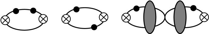
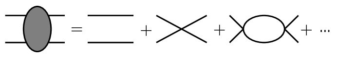
FIG. 1.: Leading order contributions to the $\nu$-$d$ scattering hadronic tensor. The gray blobs arise from no insertion plus any numbers of insertions of four nucleon operators $C_{0}^{(^{3}S_{1})}$ or $C_{0}^{(^{1}S_{0})}$, as appropriate. The crossed circles denote operators that create or annihilate two nucleons with the quantum numbers of the deuteron. The solid lines are nucleons. The solid circles correspond to insertions of leading weak current operators.

The leading order contributions to the hadronic tensor $W_{\mu\nu}$ are the diagrams shown in Fig. 1. The non-zero components of $W_{\mu\nu}$ are given by

$$W_{00}^{LO} = 2(C_{V}^{(0)^{2}}+C_{V}^{(1)^{2}})F_{1}+(C_{V}^{(0)^{2}}-C_{V}^{(1)^{2}})F_{2}+4C_{V}^{(0)^{2}}F_{3}\quad,$$ (66)

$$W_{ij}^{LO} = \delta_{ij}\left(2(C_{A}^{(0)^{2}}+C_{A}^{(1)^{2}})F_{1}+{\displaystyle{1\over 3}}(C_{A}^{(0)^{2}}-C_{A}^{(1)^{2}})F_{2}+\frac{8}{3}C_{A}^{(0)^{2}}F_{3}+\frac{4}{3}C_{A}^{(1)^{2}}F_{4}\right)\$$ (67)

$$\equiv \delta_{ij}W_{ii}^{LO}\quad,$$ (68)

with no summation implied over indexes of $W_{ii}^{LO}$. The coefficients arise from the specific forms of the single-nucleon vector and axial currents, and are given by

$$\begin{array}[!t]{ll}C_{V}^{(0)}=-\sin^{2}\vartheta_{W}&,\quad C_{V}^{(1)}={\displaystyle{1\over 2}}(1-2\sin^{2}\vartheta_{W})\quad,\\ C_{A}^{(0)}=-{\displaystyle{1\over 2}}\Delta s&,\quad C_{A}^{(1)}={\displaystyle{1\over 2}}g_{A}\quad.\end{array}$$ (69)

The functions $F_{a}$ are the individual contributions at LO from the diagrams of Fig. 1, with $F_{3}$ and $F_{4}$ both associated with the last diagram in the first row:

$$F_{1} = \text{Re}\left[{\displaystyle{2M_{N}\gamma\ p\over\pi\left[M_{N}^{2}\nu^{2}-{\bf q}^{2}p^{2}\right]}}\right]\quad,$$ (70)

$$F_{2} = \text{Re}\left[{\displaystyle{4\ \gamma\ \over\pi\nu\left|{\bf q}\right|}}\tanh^{-1}\left({\displaystyle{\left|{\bf q}\right|p\ \over M_{N}\nu}}\right)\right]\quad,$$ (71)

$$F_{3} = {\displaystyle{2\ \gamma\ \over M_{N}^{2}}}\text{Im}\left\{\left[{\displaystyle{M_{N}^{2}\ \over\pi\left|{\bf q}\right|}}\tan^{-1}\left({\displaystyle{\left|{\bf q}\right|\ \over 2(\gamma-ip)}}\right)\right]^{2}A_{-1}^{(^{3}S_{1})}(p)\right\}\quad,$$ (72)

$$F_{4} = F_{3}(^{3}S_{1}\rightarrow\ ^{1}S_{0})\ \quad.$$ (73)

The magnitude of the relative momentum between the final state proton and neutron is $p$, with

$$p=\sqrt{M_{N}\nu-\gamma^{2}-\frac{{\bf q}^{2}}{4}+i\epsilon}\quad.$$ (74)

The ‘rescattering’ amplitudes appearing in $F_{3}$ and $F_{4}$ are the leading order $NN$ scattering amplitudes in each channel, given by

$$A_{-1}^{(^{3}S_{1})}(p)={\displaystyle{-C_{0}^{(^{3}S_{1})}\over 1+{\displaystyle{M_{N}C_{0}^{(^{3}S_{1})}\ \over 4\pi}}\left(\mu+ip\right)}}\quad,$$ (75)

and similarly for the ${}^{1}S_{0}$ channel. After matching onto the effective range expansion as performed in the Appendix,

$$A_{-1}^{(^{1}S_{0})}(p)=-{\displaystyle{4\pi\over M_{N}}}{\displaystyle{1\over{\displaystyle{1\over a^{(^{1}S_{0})}}}+ip}}\quad,$$ (76)

and

$$A_{-1}^{(^{3}S_{1})}(p)=-{\displaystyle{4\pi\over M_{N}}}{\displaystyle{1\over\gamma+ip}}\quad,$$ (77)

where $a^{(^{1}S_{0})}$ is the ${}^{1}S_{0}$ channel scattering length.

From these expressions for the components of the hadronic tensor, we find that the leading contributions to the structure factors in eq.(62) are

$$W_{1}^{LO} = W_{ii}^{LO}\quad,$$ (78)

$$W_{2}^{LO} = W_{00}^{LO}+W_{ii}^{LO}\quad,$$ (79)

$$W_{3}^{LO} = 0\quad.$$ (80)

1 Elastic Limit

An important test of the inelastic calculation is that we can reproduce the elastic scattering results in the limit

$$\ \qquad p\rightarrow i\gamma+\epsilon\quad.$$ (81)

It is straightforward to see that, in this limit,

$$F_{1} = 0\quad,$$ (82)

$$F_{2} = 0\quad,$$ (83)

$$F_{3} = F_{C}^{(0)^{2}}(\left|{\bf q}\right|)\delta(\nu-{\displaystyle{{\bf q}^{2}\over 4M_{N}}})\quad,$$ (84)

$$F_{4} = 0\ \quad.$$ (85)

This, combined with eq.(62,68,80), reproduces the LO contribution to eq.(54). Further it can be shown that our NLO result also recovers the elastic limit.

2 Threshold Behavior

Another useful test of the inelastic calculation is to study the threshold behavior and compare that with the results expected from the effective range expansion. In the effective range expansion, it is well known that the dominant contribution to the threshold hadronic matrix element is the ${}^{3}S_{1}\rightarrow$ ${}^{1}S_{0}$ transition through the isovector axial coupling. The ${}^{3}S_{1}\rightarrow\,^{3}S_{1}$ transition is suppressed because amongst the NC spin-isospin operators 1, $\tau^{a}$, $\sigma^{i}$ and $\tau^{a}\sigma^{i}$: i) the isovector operators don’t contribute (the transition is isoscalar); and ii) the matrix elements of the isoscalar operators vanish in the zero recoil limit ($d$ and $np$ states are orthogonal in the zero recoil limit).

Our results reproduce these features. In the threshold limit $\omega^{{}^{\prime}},p\rightarrow 0$,

$$W_{00}^{LO} = 0\quad,$$ (86)

$$W_{ii}^{LO} = \ \left({\displaystyle{2g_{A}^{2}M_{N}p\over 3\pi\gamma^{3}}}\right)(1-a^{(^{1}S_{0})\ }\gamma)^{2}\quad.$$ (87)

Another consequence of the ${}^{3}S_{1}\rightarrow\,^{3}S_{1}$ suppression is that our results will not be sensitive to isoscalar parameters $\Delta s,$ $\mu_{s}$ and $L_{2,A}$. This has the added advantage of reducing the number of free parameters, as will be seen later.

Using eqs.(62,64,80), the differential cross-section with respect to the relative kinetic energy $E_{r}(=p^{2}/M_{N})$ between final state nucleons is

$${\displaystyle{d\sigma\over dE_{r}}} = \displaystyle\int_{-1}^{1}d(\cos\theta)2\pi{\displaystyle{d^{2}\sigma\over d\omega^{{}^{\prime}}d\Omega}}$$ (88)

$$= {\displaystyle{2G_{F}^{2}g_{A}^{2}(\omega-B)^{2}M_{N}p\over\pi^{2}\gamma^{3}}}(1-a^{(^{1}S_{0})\ }\gamma)^{2}\quad.$$ (89)

This reproduces the threshold behavior of the effective range expansion result of [5]. Our result is also consistent, at both LO and NLO, with the analytic expression of the $np\rightarrow d\gamma$ amplitude given in [28].

C Next to Leading Order

At NLO we will decompose the hadronic tensor into five components

$$W_{\mu\nu}^{NLO}=W_{\mu\nu}^{D_{2}}+W_{\mu\nu}^{L_{A}}+W_{\mu\nu}^{C_{2}}+W_{\mu\nu}^{\ \pi}+W_{\mu\nu}^{\ M_{Z}}\quad,$$ (90)

each corresponding to an insertion of a NLO ${\cal L}_{2}$ operator, single pion exchange or higher order weak couplings. Each of these five components will be considered separately.

1 D₂ Contributions

The $D_{2}$ contributions to the hadronic tensor arise from the diagrams shown in Fig. 2. They can be expressed as simple replacements of the LO results in eqs. (68,73),

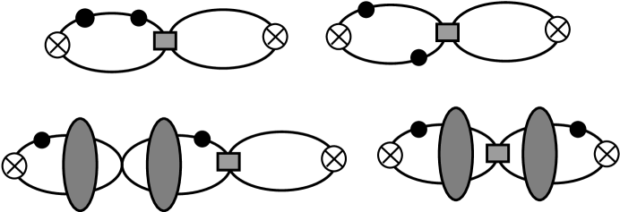
FIG. 2.: Graphs from insertions of the operators with coefficients $D_{2}^{(^{3}S_{1})}$ or $D_{2}^{(^{1}S_{0})}$ (denoted by the gray squares) that contribute to the $\nu$-$d$ scattering hadronic tensor at NLO. The gray blobs and other features are as defined in Fig. 1.

$$W_{\mu\nu}^{D_{2}}=W_{\mu\nu}^{LO}(F_{1}\rightarrow 0,F_{2}\rightarrow 0,A_{-1}^{(^{3}S_{1})}(p)\rightarrow A_{0,D_{2}}^{(^{3}S_{1})}(p),A_{-1}^{(^{1}S_{0})}(p)\rightarrow A_{0,D_{2}}^{(^{1}S_{0})}(p))\quad,$$ (91)

where

$$A_{0,D_{2}}^{(^{3}S_{1})}(p)\ =-D_{2}^{(^{3}S_{1})}m_{\pi}^{2}\left[{\displaystyle{A_{-1}^{(^{3}S_{1})}(p)\over C_{0}^{(^{3}S_{1})}}}\right]^{2}\quad,$$ (92)

and similarly for the ${}^{1}S_{0}$ channel.

2 L_A Contributions

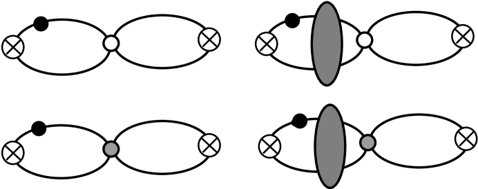
FIG. 3.: Graphs from insertions of the two-body current operators with coefficient $L_{1,A}$ (denoted by the circles) and $L_{2,A}$ (gray circles) that contribute to the $\nu$-$d$ scattering hadronic tensor at NLO. The gray blobs and other features are as defined in Fig. 1.

Diagrams with one insertion of $L_{1,A}$ or $L_{2,A}$ contribute to the hadronic tensor at NLO are shown in Fig. 3. These contribute only to the spatial piece of the hadronic tensor, and we find

$$W_{ii}^{L_{A}}=-{\displaystyle{4M_{N}\gamma(\mu-\gamma)\over 3\pi^{2}\left|{\bf q}\right|}}\text{Im}\left\{\tan^{-1}\left({\displaystyle{\left|{\bf q}\right|\ \over 2(\gamma-ip)}}\right)\left[{\displaystyle{C_{A}^{(1)}L_{1,A}\over C_{0}^{(^{1}S_{0})}}}A_{-1}^{(^{1}S_{0})}(p)+{\displaystyle{4C_{A}^{(0)}L_{2,A}\over C_{0}^{(^{3}S_{1})}}}A_{-1}^{(^{3}S_{1})}(p)\right]\right\}\quad,$$ (93)

with all other $W_{\mu\nu}^{L_{A}}=0.$

Note that the term involving $L_{1,A}$ behaves like

$${\displaystyle{\ L_{1,A}(\mu-\gamma)\over C_{0}^{(^{1}S_{0})}}}\quad,$$ (94)

which is not $\mu$–independent. The $\beta$ function of $L_{1,A}$ can be obtained by requiring the $NN\rightarrow NN\nu\overline{\nu},$ ${}^{3}S_{1}$ to ${}^{1}S_{0}$ transition amplitude to be $\mu$–independent,

$$\mu{\displaystyle{d\over d\mu}}\left({\displaystyle{L_{1,A}-C_{A}^{(1)}M_{N}(C_{2}^{(^{1}S_{0})}+C_{2}^{(^{3}S_{1})})\over C_{0}^{(^{1}S_{0})}C_{0}^{(^{3}S_{1})}}}\right)=0\quad.$$ (95)

3 C₂ Contributions

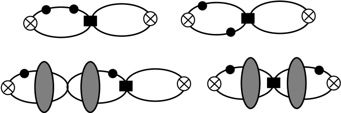
FIG. 4.: Graphs from insertions of the operator with coefficient $C_{2}^{(^{3}S_{1})}$ or $C_{2}^{(^{1}S_{0})}$ (denoted by the solid squares) that contribute to the $\nu$-$d$ scattering hadronic tensor at NLO. The gray blobs and other features are as defined in Fig. 1.

Fig. 4 shows the diagrams in which $C_{2}$ contributes to the hadronic tensor at NLO. Here we find contributions to both spatial and time-like components of the hadronic tensor

$$W_{00}^{C_{2}} = {\displaystyle{M_{N}\gamma C_{2}^{(^{3}S_{1})}(\mu-\gamma)^{2}\over 2\pi}}W_{00}^{LO}+4C_{V}^{(0)^{2}}F_{3}(A_{-1}^{(^{3}S_{1})}\rightarrow A_{0,C_{2}}^{(^{3}S_{1})})$$ (97)

$$+{\displaystyle{8C_{V}^{(0)^{2}}C_{2}^{(^{3}S_{1})}M_{N}^{2}\gamma(\mu-\gamma)\over\pi^{2}\left|{\bf q}\right|\ C_{0}^{(^{3}S_{1})}}}\text{Im}\left[A_{-1}^{(^{3}S_{1})}(p)\tan^{-1}\left({\displaystyle{\left|{\bf q}\right|\ \over 2(\gamma-ip)}}\right)\right]\quad,$$

and

$$W_{ii}^{C_{2}} = {\displaystyle{M_{N}\gamma C_{2}^{(^{3}S_{1})}(\mu-\gamma)^{2}\over 2\pi}}W_{ii}^{LO}$$ (101)

$$+{\displaystyle{8\over 3}}C_{A}^{(0)^{2}}F_{3}\left(A_{-1}^{(^{3}S_{1})}\rightarrow A_{0,C_{2}}^{(^{3}S_{1})}\right)+{\displaystyle{4\over 3}}C_{A}^{(1)^{2}}F_{4}\left(A_{-1}^{(^{1}S_{0})}\rightarrow A_{0,C_{2}}^{(^{1}S_{0})}\right)$$

$$+{\displaystyle{16C_{A}^{(0)^{2}}C_{2}^{(^{3}S_{1})}M_{N}^{2}\gamma(\mu-\gamma)\over 3\pi^{2}\left|{\bf q}\right|\ C_{0}^{(^{3}S_{1})}}}\text{Im}\left[A_{-1}^{(^{3}S_{1})}(p)\tan^{-1}\left({\displaystyle{\left|{\bf q}\right|\ \over 2(\gamma-ip)}}\right)\right]$$

$$+{\displaystyle{4C_{A}^{(1)^{2}}(C_{2}^{(^{1}S_{0})}+C_{2}^{(^{3}S_{1})})M_{N}^{2}\gamma(\mu-\gamma)\over 3\pi^{2}\left|{\bf q}\right|\ C_{0}^{(^{1}S_{0})}}}\text{Im}\left[A_{-1}^{(^{1}S_{0})}(p)\tan^{-1}\left({\displaystyle{\left|{\bf q}\right|\ \over 2(\gamma-ip)}}\right)\right]\quad,$$

where

$$A_{0,C_{2}}^{(^{3}S_{1})}(p)\ =-C_{2}^{(^{3}S_{1})}p^{2}\left[{\displaystyle{A_{-1}^{(^{3}S_{1})}(p)\over C_{0}^{(^{3}S_{1})}}}\right]^{2}\quad,$$ (102)

and similarly for the ${}^{1}S_{0}$ channel. All other $W_{\mu\nu}^{C_{2}}=0.$ An analysis using eq.(95) shows that the sum of $C_{2}$ and $L_{1,A}$ contributions to the hadronic tensor are $\mu$-independent.

4 Single Potential Pion Exchange Contributions

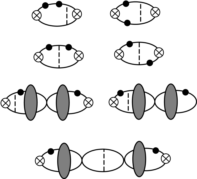
FIG. 5.: Graphs from potential pion exchange that contribute to the $\nu$-$d$ scattering hadronic tensor at NLO. The dashed lines are pions. The gray blobs and other features are as defined in Fig. 1.

The potential-pion exchange diagrams at NLO do not yield closed-form analytical solutions. However, a reasonable set of approximations could be introduced to make analytic results possible. The diagrams contributing at NLO are shown in Fig. 5. For all diagrams ${\bf q}$ dependence is neglected in the pion propagator. In the region $\omega\leq 20$ MeV that we are interested in, $\left|{\bf q}\right|\leq 40$ MeV and the error due to this approximation is estimated to be $\left\langle{\bf q}^{2}\right\rangle/m_{\pi}^{2}<10\%$. Further, for the diagrams in the second row of Fig. 5, we angle-averaged the pion propagator;

$${\frac{1}{({\bf p}-{\bf k})^{2}+m_{\pi}^{2}}}\rightarrow{\frac{1}{({\bf p}^{2}+{\bf k}^{2})+m_{\pi}^{2}}}\quad,$$ (103)

where ${\bf p}$ and ${\bf k}$ denote the nucleon momenta at the $\pi NN$ vertices. This approximation could lead to a 30% error at this order, but numerically the error is found to be of order 10%. Since the terms neglected here are formally of order NLO, we have not performed a complete calculation to NLO. But the error due to the approximations made accumulates to no more than 20% of the NLO contribution from potential pions, and is numerically an NNLO effect.

The structure factors can be decomposed in a manner similar to the LO result, with

$$\begin{array}[b]{ll}W_{00}^{\pi}&=2(C_{V}^{(0)^{2}}+C_{V}^{(1)^{2}})G_{1}+(C_{V}^{(0)^{2}}-C_{V}^{(1)^{2}})G_{2}+4C_{V}^{(0)^{2}}G_{3}\quad,\\ W_{ii}^{\pi}&=2(C_{A}^{(0)^{2}}+C_{A}^{(1)^{2}})G_{1}+{\displaystyle{1\over 3}}(C_{A}^{(0)^{2}}-C_{A}^{(1)^{2}})G_{2}+\frac{8}{3}C_{A}^{(0)^{2}}G_{3}+\frac{4}{3}C_{A}^{(1)^{2}}G_{4}\quad.\end{array}$$ (104)

The $W_{ij(i\neq j)}^{\pi}$ components are suppressed by factors of $\left\langle{\bf q}^{2}\right\rangle/m_{\pi}^{2}$ compared to the diagonal ones, so we neglect them (if they contribute at all). All other $W_{\mu\nu}^{\pi}=0$. The functions $G_{1,2}$ are simple modifications of the LO functions $F_{1,2}$, given by

$$G_{1}=F_{1}f(p)\quad,\qquad G_{2}=F_{2}f(p)\quad,$$ (105)

where

$$f(p)=-{\displaystyle{g_{A}^{2}M_{N}m_{\pi}^{2}\over 4\pi f^{2}}}\left[{\displaystyle{1\over m_{\pi}+2\gamma}}-\ \frac{1}{p}\tan^{-1}\left({\displaystyle{p\over m_{\pi}+\gamma}}\right)\right]\quad.$$ (106)

$G_{3}$ and $G_{4}$ can be further decomposed into 3 parts:

$$G_{3}=G_{3}^{(a)}+G_{3}^{(b)}+G_{3}^{(c)}\quad;\qquad G_{4}=G_{4}^{(a)}+G_{4}^{(b)}+G_{4}^{(c)}\quad.$$ (107)

with

$$\begin{array}[b]{ll}G_{3}^{(a)}&=F_{3}(A_{-1}^{(^{3}S_{1})}(p)\rightarrow A_{0,\pi}^{(^{3}S_{1})}(p))\quad,\\ G_{4}^{(a)}&=G_{3}^{(a)}(^{3}S_{1}\rightarrow\ ^{1}S_{0})\quad,\end{array}$$ (108)

where

$$\begin{array}[b]{lll}A_{0,\pi}^{(^{3}S_{1})}&={\displaystyle{g_{A}^{2}\over 2f^{2}}}\left({\displaystyle{m_{\pi}M_{N}A_{-1}^{(^{3}S_{1})}(p)\over 4\pi}}\right)^{2}\bigg{\{}&-\left({\displaystyle{\mu+ip\over m_{\pi}}}\right)^{2}\\ &&+\left[i\tan^{-1}\left({\displaystyle{2p\over m_{\pi}}}\right)-{\displaystyle{1\over 2}}\ln\left(\ {\displaystyle{m_{\pi}^{2}+4p^{2}\over\mu^{2}}}\right)+1\right]\bigg{\}}\quad.\end{array}$$ (109)

$$\begin{array}[b]{lcl}G_{3}^{(b)}&=&G_{4}^{(b)}\\ &=&-{\displaystyle{g_{A}^{2}M_{N}^{2}\gamma\over\pi^{2}f^{2}{\bf q}^{2}(m_{\pi}^{2}+2p^{2})}}\tanh^{-1}\left({\displaystyle{p\left|{\bf q}\right|\over M_{N}\nu}}\right)\\ &&\left\{p^{2}\left[\tan^{-1}\left({\displaystyle{\left|{\bf q}\right|-2p\over 2\gamma}}\right)+\tan^{-1}\left({\displaystyle{\left|{\bf q}\right|+2p\over 2\gamma}}\right)\right]+m_{\pi}^{2}\tan^{-1}\left({\displaystyle{\left|{\bf q}\right|\over 2\left(\gamma+\sqrt{m_{\pi}^{2}+p^{2}}\right)}}\right)\right\}\quad.\end{array}$$ (110)

Finally,

$$\begin{array}[]{ll}G_{3}^{(c)}=&{\displaystyle{4g_{A}^{2}M_{N}^{3}\gamma\over\pi\left|{\bf q}\right|f^{2}}}\mathop{\rm Re}\bigg{\{}\left[{\displaystyle{1\over 8\pi^{2}\left|{\bf q}\right|}}\tan^{-1}\left({\displaystyle{\left|{\bf q}\right|\over 2\left(\gamma-ip\right)}}\right)\left({\displaystyle{m_{\pi}^{2}\ \over m_{\pi}+2\gamma}}+\mu+ip\right)+h(\gamma,p)+h(-ip,i\gamma)\right]\\ &\tan^{-1}\left({\displaystyle{\left|{\bf q}\right|\over 2\left(\gamma-ip\right)}}\right)iA_{-1}^{(^{3}S_{1})}(p)\bigg{\}}\quad,\\ G_{4}^{(c)}=&G_{3}^{(c)}(^{3}S_{1}\rightarrow\ ^{1}S_{0})\quad,\end{array}$$ (111)

where

$$h(\gamma,p) = {\displaystyle{-m_{\pi}^{2}\over 16\pi^{2}(m_{\pi}+\gamma)}}\left\{-{\displaystyle{1\over\gamma-ip}}+{\displaystyle{m_{\pi}+\gamma\over\gamma^{2}+p^{2}}}\ln\left[{\displaystyle{m_{\pi}+2\gamma\over m_{\pi}+\gamma-ip\ }}\ \right]\right.$$ (113)

$$\left.+\frac{i}{\left|{\bf q}\right|}\ln\left[{\displaystyle{{\bf q}^{2}+4(\gamma^{2}+p^{2}+\left|{\bf q}\right|p)\over-{\bf q}^{2}+4(\gamma^{2}+p^{2}+i\left|{\bf q}\right|\gamma)}}\ \right]\right\}\quad.$$

5 $W_{\mu\nu}^{M_{Z}}$ Contributions

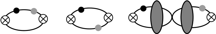
FIG. 6.: Graphs contributing to the $\nu$-$d$ scattering $W_{3}$ form factor at NLO. The dark solid circles correspond to insertions of the leading weak current operators, while the gray solid circles correspond to insertions of the next-to-leading weak magnetic moment operators. The gray blobs and other features are as defined in Fig. 1.

The diagrams with one LO single-nucleon weak current and one NLO weak magnetic moment coupling, as shown in Fig. 6, contribute to the antisymmetric part of the NLO hadronic tensor

$$W_{ij}^{M_{Z}}=-iW_{3}^{M_{Z}}\varepsilon_{0ijk}{\displaystyle{q^{k}\over M_{d}}}\quad,$$ (114)

with all other $W_{\mu\nu}^{M_{Z}}=0$. It is straightforward to show that

$$W_{3}^{M_{Z}} = -4(C_{A}^{(0)}C_{M}^{(0)}+C_{A}^{(1)}C_{M}^{(1)})F_{1}-{\displaystyle{2\over 3}}(C_{A}^{(0)}C_{M}^{(0)}-C_{A}^{(1)}C_{M}^{(1)})F_{2}$$ (116)

$$-\frac{16}{3}C_{A}^{(0)}C_{M}^{(0)}F_{3}-\frac{8}{3}C_{A}^{(1)}C_{M}^{(1)}F_{4}\quad,$$

where

$$C_{M}^{(0)}=-2\sin^{2}\vartheta_{W}\kappa^{(0)}-\frac{1}{2}\mu_{S}\quad,\quad C_{M}^{(1)}=(1-2\sin^{2}\vartheta_{W})\kappa^{(1)}\quad.$$ (117)

Recall that at LO, $W_{3}$ vanished. As such, this NLO contribution is the leading contribution to the difference between neutrino and antineutrino scattering from the deuteron.

V Antineutrino-Deuteron Charged Current Inelastic Scattering

The differential cross-section for the process

$$\overline{\nu}+d\rightarrow e^{+}+n+n$$ (118)

takes the same form as eq. (62). There are, in principle, corrections due to the finite positron mass $m_{e}$, but their impact on the total cross-section is negligible, even at threshold (they could, however, affect the angular distribution). We must also modify the phase space bounds to include the effects of the positron’s mass, as well as the neutron–proton mass splitting $\delta m=m_{n}-m_{p}$. The modified bounds are

$$\text{Max}\left[-1,-{\displaystyle{\frac{4M_{N}(\nu-B-\delta m)-\omega^{2}-\omega^{\prime 2}+m_{e}^{2}}{2\omega\sqrt{\omega^{\prime 2}-m_{e}^{2}}\ }}}\right]\leq\cos\theta\leq 1\quad,$$ (119)

$$m_{e}\leq\omega^{\prime}\leq\omega-2(M_{N}-\sqrt{M_{N}^{2}-M_{N}(B+\delta m)})\ .$$ (120)

For the most part, however, the primary difference between the neutral current and charged current cases is the fact that the charged current processes are purely isovector. As a result, the charged current structure factors can be obtained from the neutral current structure factors with the simple substitutions:

$$C_{V}^{(0)}=0\quad,\quad C_{V}^{(1)}={{{\displaystyle{\left|V_{ud}\right|\over\sqrt{2}}}}}\quad,\quad$$ (121)

$$C_{A}^{(0)}=0\quad,\quad C_{A}^{(1)}={{{\displaystyle{\left|V_{ud}\right|\over\sqrt{2}}}}}g_{A}\quad,$$ (122)

$$C_{M}^{(0)}=0\quad,\quad C_{M}^{(1)}=\sqrt{2}\left|V_{ud}\right|\kappa^{(1)}\quad,$$ (123)

$$L_{2,A}=0\quad,\quad L_{1,A}\rightarrow\sqrt{2}L_{1,A}\left|V_{ud}\right|\quad,$$ (124)

$$\nu\rightarrow\nu-\delta m\quad,$$ (125)

where we use $\left|V_{ud}\right|=0.975$ for this CKM matrix element.

VI Numerical Results

We have presented analytic expressions of the differential cross-sections ${\displaystyle{d^{2}\sigma\over d\omega^{{}^{\prime}}d\Omega}}$ for $\nu d\rightarrow\nu np$, $\bar{\nu}d\rightarrow\bar{\nu}np$ and $\bar{\nu}d\rightarrow e^{+}nn$ processes in the previous sections. These expressions have the correct elastic scattering limits and their threshold behaviors are consistent with [28]. We can now consider the numerical results for the total cross-sections of these processes. In calculating cross-sections for the different channels, we will include the isospin splitting (charge dependence) of the strong interaction in the ${}^{1}S_{0}$ channel, but it can be neglected in the weak interaction currents as a higher-order effect.

In the NLO calculations, four parameters ($\Delta s$, $\mu_{s}$, $L_{1,A}$, and $L_{2,A})$, which are not well constrained, contribute with different significance. To demonstrate their numerical effect we express the NC cross-sections at $\omega=10$ MeV as

$$\begin{array}[]{ll}\sigma(\nu(\bar{\nu})d\rightarrow\nu(\bar{\nu})np)&=0.999\pm 0.026+0.013L_{1,A}\\ &+10^{-5}\Delta s(\pm 0.5\pm 1.2\mu_{s}+6.3\Delta s-4.6L_{2,A})\quad,\end{array}$$ (126)

where $L_{1,A}$ and $L_{2,A}$ are in units of fm${}^{3}.$ It is clear, immediately, that $\Delta s$ and $\mu_{s}$ contribute less than 1% to the total cross-section. Furthermore, since dimensional analysis suggests $L_{1,A}$ and $L_{2,A}$ are of order

$$\left|L_{1,A}\right|\approx\left|L_{2,A}\right|\approx{{\displaystyle{4\pi\over M}}{\displaystyle{1\over\mu^{2}}}}\sim 5\ {\rm fm}^{3}\quad$$ (127)

at $\mu=m_{\pi}$, we see that $L_{1,A}$ could contribute at the $10\%$ level but that $L_{2,A}$ would contribute far less than 1% to the total cross-section. This agrees with the ${}^{3}S_{1}\rightarrow\,^{3}S_{1}$ suppression mentioned in section IV B 2. In this computation, $L_{1,A}$ is kept as a free parameter, $\Delta s=-0.17,$ $\mu_{s}=0$, and $L_{2,A}=0.$ The error from this choice is estimated to be less than 1%.

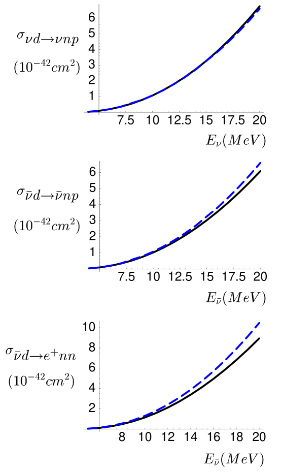
FIG. 7.: Cross-sections for $\nu d\rightarrow\nu np$ (top graph), $\bar{\nu}d\rightarrow\bar{\nu}np$ (middle graph) and $\bar{\nu}d\rightarrow e^{+}nn$ (bottom graph) shown as functions of incident $\nu(\bar{\nu})$ energy. The solid curves correspond to the average of YHH and KN results while the dashed curves correspond to the LO results in EFT. Note that at LO, there is no difference in EFT results for $\nu d\rightarrow\nu np$ and $\bar{\nu}d\rightarrow\bar{\nu}np$ cross-sections.

The LO results are parameter free, and are shown in Fig. 7 together with potential model results. With respect to the two most modern potential model calculations used, Kubodera et al.’s results (KN[2]) are persistently larger than Ying et al.’s results (YHH[1]) by 5-10% in all channels. Thus, we average the KN and YHH calculations in each channel, before comparing them to our LO results. First, consider the NC channels. At LO there is no difference in our calculation between $\nu d\rightarrow\nu np$ and $\overline{\nu}d\rightarrow\overline{\nu}np$ cross-sections. We see then that our LO result lies within 10% of the (averaged) potential model results. A similar level of agreement is seen in the comparison of our LO calculation of $\overline{\nu}d\rightarrow e^{+}nn$ to (the averaged) potential model calculations.

	$\nu d\to\nu np$		$\bar{\nu}d\to\bar{\nu}np$		$\bar{\nu}d\to e^{+}nn$
$E_{\nu(\bar{\nu})}$ MeV	a	b	a	b	a	b
4	0.0288	0.000299	0.0283	0.000299
5	0.0888	0.000965	0.0869	0.000965	0.0264	0.000268
6	0.188	0.00212	0.183	0.00212	0.111	0.00120
7	0.330	0.00381	0.319	0.00381	0.262	0.00299
8	0.516	0.00609	0.496	0.00609	0.484	0.00576
9	0.747	0.00899	0.714	0.00899	0.780	0.00960
10	1.02	0.0125	0.973	0.0125	1.15	0.0146
11	1.35	0.0167	1.27	0.0167	1.59	0.0207
12	1.72	0.0216	1.61	0.0216	2.11	0.0281
13	2.14	0.0271	2.00	0.0271	2.70	0.0368
14	2.61	0.0334	2.42	0.0334	3.35	0.0467
15	3.12	0.0404	2.88	0.0404	4.08	0.0580
16	3.69	0.0480	3.38	0.0480	4.88	0.0706
17	4.30	0.0564	3.92	0.0564	5.74	0.0846
18	4.97	0.0656	4.50	0.0656	6.68	0.0999
19	5.68	0.0754	5.12	0.0754	7.68	0.117
20	6.45	0.0860	5.77	0.0860	8.74	0.135

TABLE I.: NLO $\nu d$ and $\bar{\nu}d$ inelastic scattering results in EFT with the cross-sections written in the form $\sigma=(a+bL_{1,A})\times 10^{-42}{\rm cm}^{2}$ with $L_{1,A}$ in units of ${\rm fm}^{3}$.

Our cross-sections at NLO will have one free parameter, $L_{1,A}$. To facilitate study of the effects of this two-body contribution, we tabulate the NLO cross-sections as functions of $L_{1,A}$ in Table I. It is not surprising that we can reproduce the total cross-section results of KN and YHH in all three channels to a high degree of accuracy by choosing $L_{1,A}$ to be 6.3 fm³ and 1.0 fm³ respectively (see Fig. 8). This would imply that the 5-10% systematic errors in these two potential model calculations are due solely to different assumptions made about the short distance physics. It also suggests that EFT is a perfect tool to study the $\nu d$ breakup processes because, once $L_{1,A}$ is fixed by one experiment, predictions can be made in other channels such as the solar fusion process $pp\rightarrow de^{+}\nu$, and supernova short term cooling processes such as $np\rightarrow np\nu\overline{\nu}.$ One experiment which could, in principle, constrain $L_{1,A}$ is parity-violating $\overrightarrow{e}d\rightarrow enp$. The SAMPLE II collaboration [51] is measuring this reaction at MIT-Bates with the intent of studying the strange magnetic moment, $\mu_{s}$. Their kinematics are tuned for that purpose, and are not well-suited for an extraction of $L_{1,A}$. It would be useful to explore future possibilities that optimize an extraction of the isovector axial coupling, $L_{1,A}$.

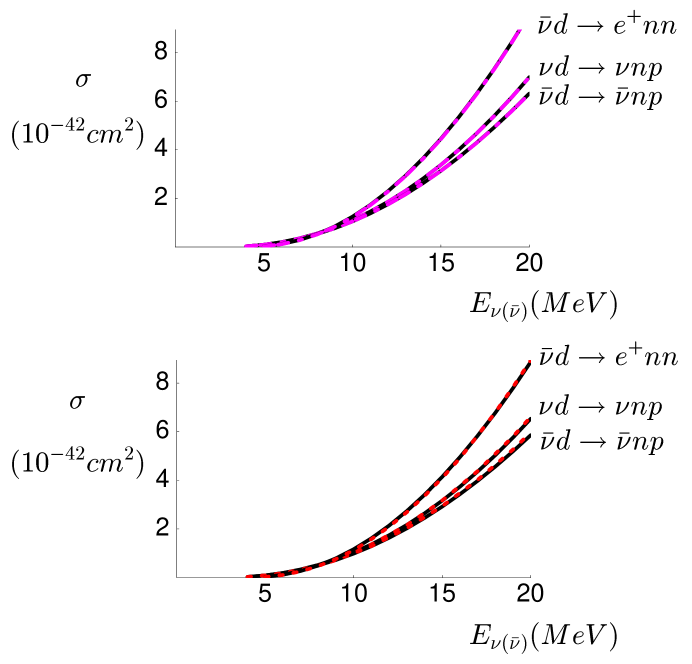
FIG. 8.: Inelastic $\nu(\bar{\nu})d$ cross-sections shown as functions of incident $\nu(\bar{\nu})$ energy. The solid curves in the upper graph are KN results while the dot-dashed curves, which lie right on top of the solid curves, are NLO results in EFT with $L_{1,A}=6.3\ {\rm fm}^{3}$. The solid curves in the lower graph are YHH results while the dashed curves, which also lie right on top of the solid curves, are NLO results in EFT with $L_{1,A}=1.0\ {\rm fm}^{3}$. In both graphs, the highest curves are $\bar{\nu}d\rightarrow e^{+}nn$ cross-sections while the middle and lower curves are $\nu d\rightarrow\nu np$ and $\bar{\nu}d\rightarrow\bar{\nu}np$ cross-sections respectively.

To make a more detailed comparison with potential model calculations, we choose the same $L_{1,A}$ values as mentioned above and plot the ratios between different calculations of the three $\nu(\overline{\nu})d$ reaction channels in Fig. 9. We find that the agreement is excellent between our calculations and the potential model results of KN (within 2%), and that we agree with the results of YHH to within 10% (the actual agreement is likely better than this – the fluctuations in YHH’s calculation may exaggerate the differences somewhat). In making these comparisons, we should recall that we have taken into account isospin splitting in the ${}^{1}S_{0}$ rescattering amplitudes for $nn$ and $np$ final states. The details can be found in the Appendix. Further, for $np$ final-states, our fit for the ${}^{1}S_{0}$ channel is not as good as for the ${}^{3}S_{1}$ channel. However, it begins to deviate from the measured phase shifts only above relative momenta of 50 MeV. The sensitivity of the calculation to these momenta is suppressed by the factor of $\omega^{\prime}|{\bf k}^{\prime}|$ in the differential cross-section for NC and CC scattering (eq. (62)). $\omega^{\prime}\propto(p_{max}^{2}-p^{2})$ means that the calculation is most sensitive to lower relative momenta.

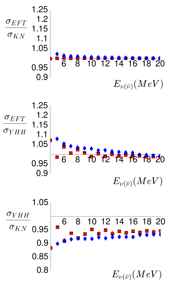
FIG. 9.: Ratios between different calculations of the inelastic $\nu(\bar{\nu})d$ cross-sections shown as functions of incident $\nu(\bar{\nu})$ energy. The first graph corresponds to $\sigma_{EFT}/\sigma_{KN}$ while the second and third graphs correspond to $\sigma_{EFT}/\sigma_{YHH}$ and $\sigma_{YHH}/\sigma_{KN}$ respectively. In all graphs, boxes are the $\nu d\to\nu np$ ratios, while triangles and diamonds are the $\bar{\nu}d\to\bar{\nu}np$ and $\bar{\nu}d\to e^{+}nn$ ratios.

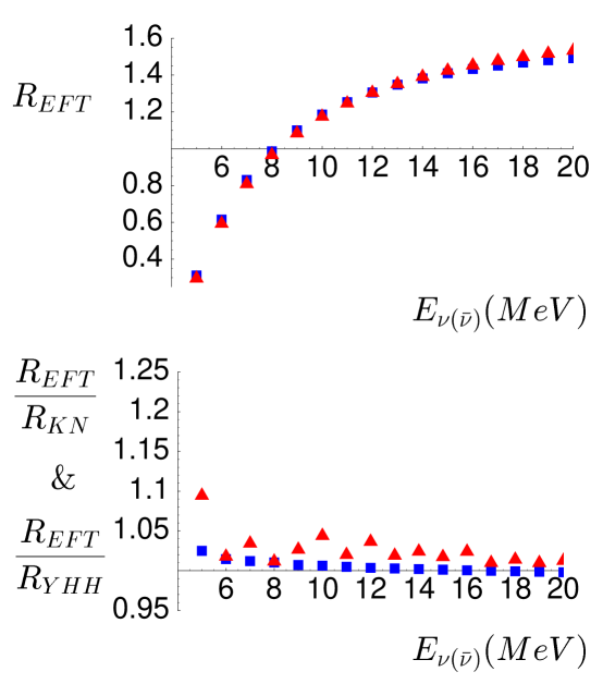
FIG. 10.: $\bar{\nu}d$ scattering CC to NC cross-section ratios $R$ shown as functions of incident $\bar{\nu}$ energy. The upper graph corresponds to the NLO EFT result with $L_{1,A}=-20~{}{\rm fm}^{3}$ (boxes) and $40~{}{\rm fm}^{3}$ (triangles). The lower graph correspond to the ratios $R_{EFT}/R_{KN}$ (boxes) and $R_{EFT}/R_{YHH}$ (triangles) with input $L_{1,A}=3.7\ {\rm fm}^{3}$ for the evaluation of $R_{EFT}$.

Another interesting quantity is the ratio $R$ between CC and NC scattering cross-sections,

$$R\equiv{\sigma_{CC}\over\sigma_{NC}}\quad.$$ (128)

This ratio is zero at threshold ($E_{\overline{\nu}}=4.03$ MeV). Above threshold, it is expected to be insensitive to the treatment or modeling of short distance physics and, in fact, changes by only $5\%$ at NLO above 5 MeV when $L_{1,A}$ varies over a wide range, from $-20$ to 40 fm³. Choosing $L_{1,A}=3.7$ fm³, our values of $R$ agree well with those obtained by KN and YHH over the full range of neutrino energies studied (Fig. 10).

One of the strengths of effective field theory is that it provides us with the ability to quantify theoretical uncertainty. It remains for us to quantify the precision of the EFT calculations presented here. Naive power counting tells us that the NLO calculation has a $10\%$ uncertainty from higher order corrections, even if we were able to fit the counterterm $L_{1,A}$ from experimental data (such as the $\overrightarrow{e}d$ scattering process mentioned earlier). This estimate is consistent with the observation that setting $L_{1,A}$ to $+6$, $0$, and $-6$ fm³ (sizes suggested from the dimensional analysis of eq. (127)) corresponds to the NLO contribution being $10$, $20$ and $30\%$ (respectively) of the LO contribution. As the NLO contribution is naively a $30\%$ effect, the NNLO effect could be estimated to be $\sim 10\%$. However, if the sign of $L_{1,A}$ is positive, as preferred by our comparison to the potential model calculations of KN and YHH, the uncertainty from NNLO could be only $\sim 4\%$. This latter scenario would also explain why we can fit the potential model results at (in general) the few percent level, given that higher order contributions are partially incorporated in very different fashions in different calculations. The size of NNLO effects will be studied further [52] using EFT without pions [42].

VII Conclusions

We have presented analytic differential cross-sections for elastic and inelastic neutrino deuteron scattering processes using effective field theory. For elastic scattering, the deuteron axial form factor arising from strange matrix elements, and the deuteron strange magnetic moment form factor are computed to NLO with two-body current dependence. For inelastic scattering, two neutral current processes $\nu d\rightarrow\nu np$, $\overline{\nu}d\rightarrow\overline{\nu}np$ and one charge current process $\overline{\nu}d\rightarrow e^{+}nn$ are computed to NLO with an isovector axial two-body matrix element whose value is yet to be fixed by experiment. Potential model calculations done by Kubodera et al. and Ying et al. are reproduced, with a high degree of accuracy, by choosing different values for the two-body matrix element. This implies that the differences between the two potential model calculations lie in their treatment of short distance physics. The charged current to neutral current $\overline{\nu}d$ cross-section ratio is confirmed to be insensitive to short distance physics, and the same ratio is obtained by potential models and this calculation within our intrinsic uncertainties (conservatively estimated to be 5%) for the full range of incident neutrino energies studied, up to 20 MeV. The two-body matrix element could be fixed using the parity-violating process $\overrightarrow{e}d\rightarrow enp$.

There still remains the need to calculate the other charged current process, $\nu d\rightarrow e^{-}pp$, in EFT. This is the primary reaction channel at SNO and issues of its precision and accuracy should not be simply inferred from the processes studied here. The complications introduced because of coulomb interactions in the final state make it more appropriate to discuss this process elsewhere [53], along with details of the angular distributions of the charged-current reactions [54].

ACKNOWLEDGMENTS

We would like to thank Martin Savage, Doug Beck, Elizabeth Beise, Wick Haxton, Sanjay Reddy, Hamish Robertson, and Roxanne Springer for useful discussions. This work is supported, in part, by the U.S. Dept. of Energy under Grant No. DE-FG03-97ER4014. M.B. is supported by a grant from the Natural Sciences and Engineering Research Council of Canada.

APPENDIX

This appendix summarizes how the $NN$ scattering strong interaction parameters can be fit to phase shift data by matching onto the effective range expansion (ERE). The $NN$ scattering amplitude ${\cal A}$ has a power series expansion in $Q$; ${\cal A}={\cal A}_{-1}+{\cal A}_{0}+...$, where the subscripts denote the powers in $Q$. ${\cal A}_{-1}$ and ${\cal A}_{0}$ have been calculated in [21]. The standard parameterization of the $NN$ scattering amplitude is given by

$${\cal A}=\frac{4\pi}{M_{N}}\frac{1}{p\cot\delta-ip}\quad.$$ (129)

where $p$ is the relative momentum and $\delta$ is the phase shift. The effective range expansion is a power series expansion of $p\cot\delta$, yielding

$$p\cot\delta=-\frac{1}{a}+\frac{1}{2}r_{0}p^{2}+\cdots\quad,$$ (130)

where $a$ is the scattering length and $r_{0}$ is the effective range. For the ${}^{1}S_{0}$ channel, we can rewrite eq. (129) as

$${\cal A}^{ERE} = -\frac{4\pi}{M_{N}}\frac{1}{\left(\frac{1}{a^{(^{1}S_{0})}}+ip\right)}\left[1+\frac{1}{2}\frac{r_{0}^{(^{1}S_{0})}p^{2}}{\left(\frac{1}{a^{(^{1}S_{0})}}+ip\right)}+\cdots\right]\quad$$ (131)

$$= {\cal A}_{-1}^{ERE}+{\cal A}_{0}^{ERE}+...\quad,$$ (132)

where we have performed a $Q$-expansion. At LO, we can relate the coefficient $C_{0}^{{}^{1}S_{0}}$ to effective range parameters through equating

$${\cal A}_{-1}(p)={\cal A}_{-1}^{ERE}(p)$$ (133)

yielding

$$C_{0}^{(^{1}S_{0})}(\mu)=-\frac{4\pi}{M_{N}}\frac{1}{\left(\mu-{1\over a^{{}^{1}S_{0}}}\right)}\quad.$$ (134)

At NLO, ${\cal A}_{0}$ does not have the same $p$ dependence as ${\cal A}_{0}^{ERE}.$ The NLO matching is performed near $p=0$. As $p\rightarrow 0,$

$${\cal A}^{ERE}_{0}(p)\rightarrow-\frac{2\pi}{M_{N}}a^{(^{1}S_{0})^{2}}r_{0}^{(^{1}S_{0})}p^{2}\quad.$$ (135)

The matching yields

$$D_{2}^{(^{1}S_{0})}(m_{\pi})=0\ \quad,$$ (136)

and

$$C_{2}^{(^{1}S_{0})}(m_{\pi})=\frac{2\pi}{M_{N}}\frac{r_{0}^{(^{1}S_{0})}}{\left(m_{\pi}-\frac{1}{a^{(^{1}S_{0})}}\right)^{2}}-\frac{g_{A}^{2}\left(3a^{(^{1}S_{0})^{2}}m_{\pi}^{2}-8a^{(^{1}S_{0})}m_{\pi}+6\right)}{6f^{2}a^{(^{1}S_{0})^{2}}m_{\pi}^{2}\left(m_{\pi}-\frac{1}{a^{(^{1}S_{0})}}\right)^{2}}\ \quad.$$ (137)

The ERE parameters

$$\begin{array}[!t]{ll}a_{np}=-23.714\pm 0.013\text{ fm}&,\quad r_{0_{np}}=2.73\pm 0.03\text{ fm}\quad,\\ a_{nn}=-18.5\pm 0.4\text{ fm}&,\quad r_{0_{nn}}=2.80\pm 0.11\text{ fm}\quad,\end{array}$$ (138)

are different between n-p and n-n systems [55]. Taking into account this observed violation of charge independence, we find for the n-p system

$$C_{0}^{(^{1}S_{0})}(m_{\pi})=-3.56\text{ fm}^{2}\quad,\quad D_{2}^{(^{1}S_{0})}(m_{\pi})=0\text{ fm}^{4}\quad,\quad C_{2}^{(^{1}S_{0})}(m_{\pi})=2.79\text{ fm}^{4}\quad,$$ (139)

while for the n-n system

$$C_{0}^{(^{1}S_{0})}(m_{\pi})=-3.50\text{ fm}^{2}\quad,\quad D_{2}^{(^{1}S_{0})}(m_{\pi})=0\text{ fm}^{4}\quad,\quad C_{2}^{(^{1}S_{0})}(m_{\pi})=2.71\text{ fm}^{4}\quad.$$ (140)

For the ${}^{3}S_{1}$ system, $p\cot\delta$ is usually expanded around the deuteron pole,

$$p\cot\delta=-\gamma+\frac{1}{2}r_{0}^{(^{3}S_{1})}(p^{2}+\gamma^{2})+\cdots\quad,$$ (141)

such that we can rewrite eq.(129) as

$${\cal A}^{ERE} = \frac{4\pi}{M_{N}}\frac{1}{-\gamma-ip\ }\left[1+\frac{1}{2}r_{0}^{(^{3}S_{1})}(\gamma-ip)+\cdots\right]$$ (142)

$$= {\cal A}_{-1}^{ERE}+{\cal A}_{0}^{ERE}+...\quad,$$ (143)

after performing a $Q$-expansion. The LO matching yields

$$C_{0}^{(^{3}S_{1})}(\mu)=-\frac{4\pi}{M_{N}}\frac{1}{\left(\mu-\gamma\right)}\quad.$$ (144)

At NLO, the matching is performed at $p=0$ and $i\gamma$, so that the scattering length is reproduced and the residue of the deuteron pole is not changed in the NLO EFT amplitude. That yields two conditions

$${\cal A}_{-1}(0)+{\cal A}_{0}(0)=-\frac{4\pi a^{(^{3}S_{1})}}{M_{N}}\quad,$$ (145)

$${\cal A}_{0}(i\gamma)={\cal A}_{0}^{ERE}(i\gamma)=0\quad.$$ (146)

Matching at $\mu=m_{\pi}$, these two conditions can be solved for the coefficients $D_{2}^{{}^{3}S_{1}}$ and $C_{2}^{{}^{3}S_{1}}$

$$D_{2}^{(^{3}S_{1})}(m_{\pi})=-\frac{4\pi}{M_{N}}\frac{\gamma\left(1-a^{(^{3}S_{1})}\gamma\right)}{m_{\pi}^{2}\left(m_{\pi}-\gamma\right)^{2}}\quad,$$ (147)

and

$$C_{2}^{(^{3}S_{1})}(m_{\pi})=\frac{1}{2\gamma^{2}\ }\left[\left(2D_{2}^{(^{3}S_{1})}(m_{\pi})m_{\pi}^{2}+\frac{g_{A}^{2}}{f^{2}}\right)+\frac{g_{A}^{2}m_{\pi}^{2}}{f^{2}\left(m_{\pi}-\gamma\right)^{2}}\left(\ln\frac{m_{\pi}+2\gamma}{m_{\pi}}-1\right)\right]\ \quad.$$ (148)

Numerically we find

$$C_{0}^{(^{3}S_{1})}(m_{\pi})=-5.64\text{ fm}^{2}\quad,\quad D_{2}^{(^{3}S_{1})}(m_{\pi})=1.46\text{ fm}^{4}\quad,\quad C_{2}^{(^{3}S_{1})}(m_{\pi})=10.05\text{ fm}^{4}\quad.$$ (149)

The fit to the n-p scattering phase shifts is shown in Fig. 11.

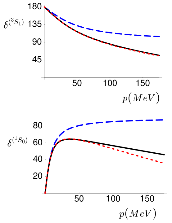
FIG. 11.: n-p scattering phase shifts (measured in degrees) for the ${}^{3}S_{1}$ (upper graph) and ${}^{1}S_{0}$ channels (lower graph). The dashed curves are the LO results and the solid curves are the NLO results from eqs.(149,139). The dotted curves are the results of the Nijmegen partial wave analysis.

REFERENCES

- [1] S. Ying, W.C. Haxton, and E. M. Henley, Phys. Rev. C 45, 1982 (1992); Phys. Rev. D 40, 3211 (1989).
- [2] K. Kubodera and S. Nozawa, Int. J. Mod. Phys. E3, 101 (1994); Y. Kohyama and K. Kubodera, USC(NT)-Report-92-1, 1992, unpublished.
- [3] S.D. Ellis and J.N. Bahcall, Nucl. Phys. A 114, 636 (1968).
- [4] A. Ali and C.A. Dominguez, Phys. Rev. D 12, 3673 (1975).
- [5] H. C. Lee, Nucl. Phys. A 294, 473 (1978).
- [6] S.L. Glashow, Nucl. Phys. 22, 579 (1961); S. Weinberg, Phys. Rev. Lett. 19, 1264 (1967); A. Salam, in Nobel Symposium, No. 8, ed. N. Svartholm (Almquist and Wiksells, Stockholm, 1968).
- [7] G.A. Aardsma et al., Phys. Lett. B 194, 321 (1987).
- [8] G.T. Ewan et al., SNO proposal SNO-87-12, 1987.
- [9] J.N. Bahcall, Kubodera, and S. Nozawa, Phys. Rev. D 38, 1030 (1987).
- [10] N. Tatara, Y. Kohyama and K. Kubodera, Phys. Rev. C 42, 1694 (1990).
- [11] M. Doi and K. Kubodera, Phys. Rev. C 45, 1988 (1992).
- [12] S. Weinberg, Phys. Lett. B 251, 288 (1990); Nucl. Phys. B 363, 3 (1991); Phys. Lett. B 295, 114 (1992).
- [13] C. Ordonez and U. van Kolck, Phys. Lett. B 291, 459 (1992); C. Ordonez, L. Ray and U. van Kolck, Phys. Rev. Lett. 72, 1982 (1994); Phys. Rev. C 53, 2086 (1996); U. van Kolck, Phys. Rev. C 49, 2932 (1994).
- [14] J. Friar, nucl-th/9601012; nucl-th/9601013; Few Body Systems Suppl. 99, 1 (1996); nucl-th/9804010; J.L. Friar, D. Huber, and U. van Kolck, Phys. Rev. C 59, 53 (1999).
- [15] T.-S. Park, D.-P. Min and M. Rho, Phys. Rev. Lett. 74, 4153 (1995) ; Nucl. Phys. A 596, 515 (1996).
- [16] T.D. Cohen, Phys. Rev. C 55, 67 (1997). D.R. Phillips and T.D. Cohen, Phys. Lett. B 390, 7 (1997). K.A. Scaldeferri, D.R. Phillips, C.W. Kao and T.D. Cohen, Phys. Rev. C 56, 679 (1997). S.R. Beane, T.D. Cohen and D.R. Phillips, nucl-th/9709062; D.R. Phillips, S.R. Beane and T.D. Cohen, Annals Phys. 263, 255 (1998).
- [17] M.J. Savage, Phys. Rev. C 55, 2185 (1997).
- [18] G.P. Lepage, nucl-th/9706029, Lectures at 9th Jorge Andre Swieca Summer School: Particles and Fields, Sao Paulo, Brazil, Feb 1997.
- [19] M. Luke and A.V. Manohar, Phys. Rev. D 55, 4129 (1997).
- [20] D.B. Kaplan, M.J. Savage, and M.B. Wise, Nucl. Phys. B 478, 629 (1996).
- [21] D.B. Kaplan, M.J. Savage and M.B. Wise, Phys. Lett. B 424, 390 (1998); Nucl. Phys. B 534, 329 (1998).
- [22] U. van Kolck, Nucl. Phys. A 645, 273 (1999)
- [23] D.B. Kaplan, M.J. Savage and M.B. Wise, Phys. Rev. C 59, 617 (1999).
- [24] J.W. Chen, H. W. Griesshammer, M. J. Savage and R. P. Springer, Nucl. Phys. A 644, 221 (1999);Nucl. Phys. A 644, 245 (1999).
- [25] J.W. Chen, nucl-th/9810021, to appear in Nucl. Phys. A..
- [26] M. J. Savage and R.P. Springer, Nucl. Phys. A 644, 235 (1999).
- [27] D. B. Kaplan, M. J. Savage, R. P. Springer and M. B. Wise, Phys. Lett. B 449, 1 (1999).
- [28] M. J. Savage, K. A. Scaldeferri, Mark B.Wise, nucl-th/9811029.
- [29] T. Mehen and I.W. Stewart, nucl-th/9901064; nucl-th/9809095; Phys. Lett. B 445, 378 (1999).
- [30] G. Rupak and N. Shoresh, nucl-th/9902077.
- [31] J. Gegelia, Phys. Lett. B 429, 227 (1998); nucl-th/9806028; nucl-th/9805008; nucl-th/9802038;
- [32] A. K. Rajantie, Nucl. Phys. B 480, 729 (1996).
- [33] J.V. Steele and R.J. Furnstahl, Nucl. Phys. A 637, 46 (1998); Nucl. Phys. A 645, 439 (1999).
- [34] T.D. Cohen and J.M. Hansen, Phys. Rev. C 59, 13 (1999); nucl-th/9901065.
- [35] T.-S. Park, K. Kubodera, D.-P. Min, and M. Rho, Phys. Rev. C 58, 637 (1998); nucl-th/9807054; astro-ph/9804144.
- [36] X. Kong and F. Ravndal, nucl-th/9803046; Phys. Lett. B 450, 320 (1999); nucl-th/9903523; nucl-th/9904066.
- [37] E. Epelbaoum and U.G. Meissner, nucl-th/9902042; E. Epelbaoum, W. Glockle, A. Kruger and Ulf-G. Meissner, Nucl. Phys. A 645, 413 (1999); E. Epelbaoum, W. Glockle and Ulf-G. Meissner, Phys. Lett. B 439, 1 (1998); E. Epelbaoum, W. Glockle and Ulf-G. Meissner, Nucl. Phys. A 637, 107 (1998).
- [38] T. Mehen, I. W. Stewart and M.B. Wise, hep-ph/9902370.
- [39] D. R. Phillips, S. R. Beane and M. C. Birse, hep-ph/9810049.
- [40] P.F. Bedaque, H.W. Hammer and U. van Kolck, Phys. Rev. Lett. 82, 463 (1999); Phys. Rev. C 58, R641 (1998); P.F. Bedaque and U. van Kolck, Phys. Lett. B 428, 221 (1998).
- [41] T.-S. Park, K. Kubodera, D.-P. Min and M. Rho, Talk presented by M. Rho at the Nuclear Physics with Effective Field Theory: 1999 workshop, INT, University of Washington, Seattle, February 1999. nucl-th/9904053.
- [42] J.W. Chen, G. Rupak and M.J. Savage nucl-th/9902056, to appear in Nucl. Phys. A.; nucl-th/9905009.
- [43] S.R. Beane, M. Malheiro, D.R. Phillips and U. van Kolck nucl-th/9905023.
- [44] D.B. Kaplan and J.V. Steele, nucl-th/9905027.
- [45] K. Abe et al., Phys. Rev. Lett. 74, 346 (1995).
- [46] D. Adams et al., Phys. Lett. B 329, 399 (1994); Phys. Lett. B 339, 332 (1994); Phys. Lett. B 357, 248 (1995).
- [47] M.J. Savage and J. Walden, Phys. Rev. D 55, 5376 (1997).
- [48] T. Frederico, E.M. Henley, S.J. Pollock, and S. Ying, Phys. Rev. C 46, 347 (1992).
- [49] B. Mueller et al., Phys. Rev. Lett. 78, 3824 (1997).
- [50] M.J. Musolf et al., Phys. Rep. 239, 1 (1994).
- [51] Bates experiment # 94-11 (M. Pitt and E.J. Beise, contacts).
- [52] M.N. Butler and J.W. Chen, in preparation.
- [53] M.N. Butler, J.W. Chen, and X. Kong, in preparation.
- [54] P. Vogel and J.F. Beacom, hep-ph/9903554.
- [55] S.A. Coon, nucl-th/9903033.